Rain evaporation, snow melt and entrainment at the heart of water vapor isotopic variations in the tropical troposphere, according to large-eddy simulations and a two-column model

HAL Id: hal-03025845

https://hal.archives-ouvertes.fr/hal-03025845

Submitted on 26 Nov 2020

HAL is a multi-disciplinary open access

archive for the deposit and dissemination of

sci-entific research documents, whether they are

pub-lished or not. The documents may come from

teaching and research institutions in France or

abroad, or from public or private research centers.

L’archive ouverte pluridisciplinaire HAL, est

destinée au dépôt et à la diffusion de documents

scientifiques de niveau recherche, publiés ou non,

émanant des établissements d’enseignement et de

recherche français ou étrangers, des laboratoires

publics ou privés.

Rain evaporation, snow melt and entrainment at the

heart of water vapor isotopic variations in the tropical

troposphere, according to large-eddy simulations and a

two-column model

Camille Risi, Caroline Muller, Peter Blossey

To cite this version:

Camille Risi, Caroline Muller, Peter Blossey. Rain evaporation, snow melt and entrainment at the

heart of water vapor isotopic variations in the tropical troposphere, according to large-eddy simulations

and a two-column model. Journal of Advances in Modeling Earth Systems, American Geophysical

Union, In press. �hal-03025845�

Rain evaporation, snow melt and entrainment at the heart of water

1

vapor isotopic variations in the tropical troposphere, according to

2

large-eddy simulations and a two-column model

3

Camille Risi

1

_{, Caroline Muller}

1

_{, Peter N. Blossey}

2

4

September 15, 2020

5

1 _{Laboratoire de Météorologie Dynamique, IPSL, CNRS, Sorbonne Université, Paris, France}

6

2 _{Department of Atmospheric Sciences, University of Washington, Seattle, USA}

7 8

(<=140 characters)

9

1. Rain evaporation enriches the tropospheric water vapor more if more snow sublimates before melting and

10

more rain evaporates.

11

2. Entrainment of dry air reduces the vertical isotopic gradient and limits the tropospheric depletion of water

12

vapor.

13

3. These mechanisms explain the increased depletion of tropospheric water vapor as tropospheric relative

hu-14 midity increases. 15

Abstract

16 (<=250 words) 17 18

The goal of this study is twofold. First, we aim at developing a simple model as an interpretative framework

19

for the water vapor isotopic variations in the tropical troposphere over the ocean. We use large-eddy simulations

20

to justify the underlying assumptions of this simple model, to constrain its input parameters and to evaluate its

21

results. Second, we aim at interpreting the depletion of the water vapor isotopic composition in the lower and

mid-22

troposphere as precipitation increases, which is salient features in tropical oceanic observations. This constitutes

23

a stringent test on the relevance of our interpretative framework. Previous studies, based on observations or

24

models with parameterized convection, have highlighted the roles of deep convective and meso-scale downdrafts,

25

rain evaporation, rain-vapor diffusive exchanges and mixing processes.

26

The interpretative framework that we develop is a two-column model representing the net ascent in clouds and

27

the subsiding environment. We show that the mechanisms for depleting the troposphere when precipitation rate

28

is larger all stem from the higher tropospheric relative humidity. First, when the relative humidity is larger, less

29

snow sublimates before melting and a smaller fraction of rain evaporates. Both effects lead to more depleted rain

30

evaporation and eventually more depleted water vapor. This mechanism dominates in regimes of large-scale ascent.

31

Second, the entrainment of dry air into clouds reduces the vertical isotopic gradient and limits the tropospheric

32

depletion of water vapor. This mechanism dominates in regimes of large-scale descent.

33

Contents

34

1 Introduction 2

35

1.1 Looking for an interpretative framework for water vapor isotopic profiles . . . 2

36

1.2 Large-eddy simulation analysis as a guide to design the interpretative framework . . . 3

37

1.3 Interpreting the amount effect . . . 3

2 Large-eddy simulations 4

39

2.1 Model and simulations . . . 4

40

2.2 Simulated amount effect and basic features . . . 5

41

2.3 Steepness of the q − δDv relationship . . . 5

42

2.4 Effect of de-activating rain-vapor exchanges . . . 6

43

2.5 Vertical profiles binned by moist static energy . . . 6

44

2.6 Vertical profiles for cloudy regions and for the environment . . . 11

45

2.7 What controls the isotopic composition of the rain evaporation flux? . . . 12

46

2.8 Summary . . . 13

47

3 A simple two-column model to quantify the relative contributions of different processes 13

48

3.1 Model equations and numerical application to LES outputs . . . 13

49

3.1.1 Balance equations . . . 13

50

3.1.2 Other simplifying assumptions and differential equations . . . 15

51

3.1.3 Numerical solutions . . . 16

52

3.1.4 Diagnosed input parameters . . . 17

53

3.1.5 Closure in the sub-cloud layer . . . 17

54

3.1.6 Evaluation of the two-column model . . . 19

55

3.2 Decomposition of relative humidity and δD variations . . . 19

56

3.2.1 Decomposition of relative humidity . . . 19

57 3.2.2 Dilution effect on δD . . . 19 58 3.2.3 Decomposition of δD . . . 22 59 4 Conclusion 23 60 4.1 Summary . . . 23 61 4.2 Discussion . . . 24 62 4.3 Perspectives . . . 26 63

1

Introduction

64

1.1

Looking for an interpretative framework for water vapor isotopic profiles

65

The isotopic composition of water vapor (e.g. its Deuterium content, commonly expressed as δD = (R/RSMOW−1)×

66

1000 in h, where R is the ratio of Deuterium over Hydrogen atoms in the water, and SMOW is the Standard Mean

67

Ocean Water reference) evolves along the water cycle as phase changes are associated with isotopic

fractiona-68

tion. Consequently the isotopic composition of precipitation recorded in paleoclimate archives has significantly

69

contributed to the reconstruction of past hydrological changes ([Wang et al., 2001]). It has also been suggested

70

that observed isotopic composition of water vapor could help better understand atmospheric processes and evaluate

71

their representation in climate models, in particular convective processes ([Schmidt et al., 2005, Bony et al., 2008,

72

Lee et al., 2009, Field et al., 2014]). Yet, water isotopes remain rarely used beyond the isotopic community to

an-73

swer today’s pressing climate questions. A prerequisite to better assess the strengths and weaknesses of the isotopic

74

tool is to better understand what controls spatio-temporal variations in water vapor isotopic composition (δDv)

75

through the tropical troposphere, in particular how convective processes drive these variations.

76

While there are interpretative frameworks for the controls of free tropospheric humidity ([Sherwood, 1996,

77

Romps, 2014]), no such interpretative framework exist for water isotopes beyond the simple Rayleigh distillation or

78

mixing lines ([Worden et al., 2007, Bailey et al., 2017]). We aim at filling this gap here. The first goal of this paper

79

is thus to design an interpretative framework that could be useful in the future to interpret water vapor isotopic

80

variations in the tropical troposphere in a wide range of contexts. Analogous to that for relative humidity, this

81

framework will also allow us to compare the processes controlling relative humidity and isotopic composition.

82

Frameworks do exist to interpret the δDv in the sub-cloud layer (SCL), such as the [Merlivat and Jouzel, 1979]

83

closure assumption, later extended to account for updrafts and downdrafts ([Risi et al., 2020]). This latter

frame-84

work highlighted the need to know the steepness of the relationship between δDv and humidity q as they evolve

85

with altitude. This motivates us to develop a framework that allows us to predict the δDv evolution with altitude

86

in the troposphere.

1.2

Large-eddy simulation analysis as a guide to design the interpretative framework

88

Many previous studies investigating the processes controlling tropospheric δDv have relied on general circulation

89

models that include convective parameterization ([Lee et al., 2007, Bony et al., 2008, Risi et al., 2008, Field et al., 2010]).

90

However, parameterizations include numerous simplifications or assumptions that are responsible for a significant

91

part of biases in the present climate simulated by GCMs and of inter-model spread in climate change projections

92

([Randall et al., 2003, Stevens and Bony, 2013, Webb et al., 2015]). Here, we thus use large-eddy simulations (LES)

93

as a guide to design the interpretative framework. These high-resolution simulations allows us to explicitly resolve

94

convective motions. These simulations will also provide the input parameters for our interpretative framework, and

95

a benchmark to evaluate its results.

96

1.3

Interpreting the amount effect

97

In the tropics, it has long been observed that in average over a month or longer, the isotopic composition of

98

the rain is more depleted when the precipitation rate is stronger ([Dansgaard, 1964, Rozanski et al., 1993]). This

99

phenomenon is called the “amount effect”. Since most of the precipitation in the tropics is associated with deep

100

convection, understanding the amount effect is a stringent test on our understanding of how convective processes

101

affect the water vapor isotopic composition trough the tropical troposphere. The capacity of our interpretative

102

framework to predict the amount effect will thus be a stringent test on its relevance. The second goal of this study

103

is thus to better understand the processes underlying the amount effect, using the interpretative framework.

104

[Dansgaard, 1964] hypothesized that the amount effect could be due to the progressive depletion by convective

105

storms of the vapor from which the rain forms, and to rain evaporation and diffusive exchanges between the

106

rain and the vapor. If the case, the amount effect crucially depends on the isotopic composition of the vapor.

107

From a column-integrated water budget perspective, the isotopic composition of precipitation depends on the

108

relative proportion of the precipitation that originates from horizontal advection and from surface evaporation

109

([Lee et al., 2007, Moore et al., 2014]). More precipitation is generally associated with more large-scale ascent and

110

thus more large-scale convergence. Since vapor from horizontal advection is more depleted than water from surface

111

evaporation because it has already been processed in clouds, the precipitation is more depleted. In this view as

112

well, the amount effect crucially depends on the isotopic composition of the vapor.

113

Water isotopic measurements in the vapor phase, by satellite or in-situ, have confirmed that increased

precip-114

itation was associated with more depleted water vapor ([Worden et al., 2007, Kurita, 2013, Lacour et al., 2017]).

115

Hereafter we will call this the “vapor amount effect”. Actually, the precipitation and water vapor isotopic

composi-116

tion often vary in concert ([Kurita, 2013, Tremoy et al., 2014]). In this paper, we will thus focus on understanding

117

the processes underlying the “vapor amount effect”.

118

From previous studies, four hypotheses have emerged to explain the “vapor amount effect”:

119

1. Hypothesis 1: As precipitation rate increases, convective or meso-scale downdrafts bring more depleted vapor

120

from above into the sub-cloud layer (SCL) ([Risi et al., 2008, Kurita et al., 2011, Kurita, 2013]). This is

121

because the water vapor δD (δDv) generally decreases with altitude, because as water vapor is lost through

122

condensation and specific humidity q decreases, heavy isotopes are preferentially lost in the condensed phase.

123

This phenomenon is called Rayleigh distillation and is plotted in a q−δDvdiagram in Figure 1 (blue). However,

124

downdrafts would both decrease δDv and q. This hypothesis is thus inconsistent with the observation that q

125

generally increases while δDv decreases as precipitation rate increases. By itself, this hypothesis cannot be

126

sufficient.

127

2. Hypothesis 2: As precipitation rate increases, the moistening effect by rain evaporation increases. If rain

128

evaporation is more depleted than the vapor, then it depletes the vapor ([Worden et al., 2007]). The effect

129

of rain evaporation is represented in purple in Figure 1. If the evaporated fraction of the rain is small, rain

130

evaporation acts to deplete the vapor because light isotopes preferentially evaporate.

131

3. Hypothesis 3: As precipitation rate increases, the rain evaporation is more depleted. For example, if

precipi-132

tation rate increases, the fraction of rain that evaporates is smaller, which leads the evaporation to be more

133

depleted ([Risi et al., 2008, Risi et al., 2010, Tremoy et al., 2014, Risi et al., 2020], Figure 1, purple).

Alter-134

natively, larger precipitation rates typically occur in moister environments, which favors rain-vapor diffusive

135

exchanges rather than pure evaporation [Lawrence et al., 2004, Lee and Fung, 2008]. Since rain comes from

136

higher altitudes, it is more depleted than if in equilibrium with the local vapor, and thus rain-vapor diffusive

137

exchanges favor more depleted evaporation.

−120 −80 −160 −200 1.4 1.8 2.2 2.6 3

0km

3km

5km

in−situ condensation

dehydration by mixing

droplet evaporation

rain reevaporation

ln(q) ()

ln

(R

)

·1

00

0

(

h

)

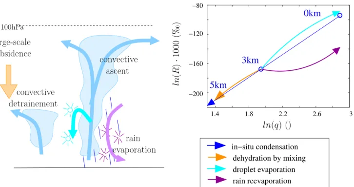
100hPa

large-scale

subsidence

convective

detrainement

convective

ascent

rain

evaporation

Figure 1: Schematic showing the influence of different processes on q and δDv. Condensation and immediate loss of condensate in convective updrafts leads to drying and depleting the water vapor following Rayleigh distillation (blue). During evaporation of cloud droplets, each droplet evaporates totally. Since cloud droplets are enriched in heavy isotopes, this moistens the air and enriches the vapor (cyan). In contrast, during evaporation of rain drops, each drop evaporates progressively. Whereas it moistens the air, it depletes the vapor for small evaporation fractions and enriches the vapor for large evaporation fraction (purple). Finally, mixing of subsiding air with air detrained from convective updrafts dehydrates the air and depletes the vapor following a hyperbolic curve, leading to higher δDv for a given q compared to Rayleigh (orange). The curves are plotted following simple Rayleigh and mixing lines with approximate values taken from the control LES described later in the article.

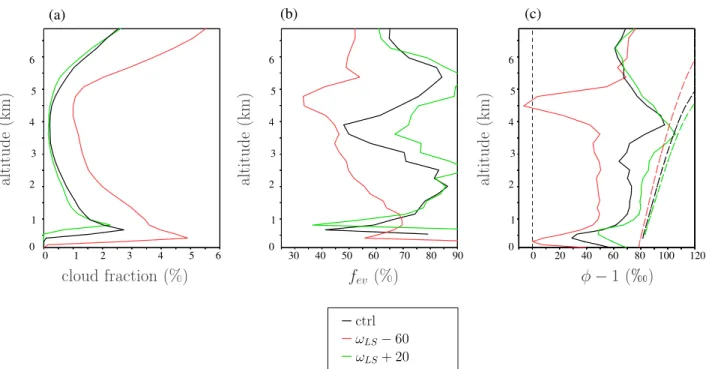
4. Hypothesis 4: As precipitation rate increases, dehydration by mixing dominates relatively to dehydration

139

by condensation. Due to the hyperbolic shape of the mixing lines in a q − δD diagram, dehydration by

140

mixing with a dry source is associated with a smaller depletion than predicted by Rayleigh distillation

141

[Dessler and Sherwood, 2003, Galewsky and Hurley, 2010, Galewsky and Rabanus, 2016] (Figure 1 orange).

142

[Bailey et al., 2017] argues that in more subsiding regions, mid-tropospheric vapor is more enriched for a

143

given specific humidity because air masses result from the mixing between air subsiding from a higher altitude

144

and shallow convective detrainment.

145

We notice that hypothesis 2-4 are all associated with an increased steepness as precipitation rate increases (Figure

146

1), consistent with the key role of the steepness of the q − δDv relationship in depleting the SCL water vapor

147

highlighted by [Risi et al., 2020]. The mechanisms underlying these hypotheses will thus have to be key ingredients

148

of our interpretative framework.

149

The LES will be described and analyzed in section 2. The interpretative framework will be designed and used

150

to interpret the “vapor amount effect” in section 3. Finally, section 4 will offer a summary, some discussion and

151

perspectives.

152

2

Large-eddy simulations

153

2.1

Model and simulations

154

We use the same LES model as in [Risi et al., 2020], namely the System for Atmospheric Modeling (SAM)

non-155

hydrostatic model ([Khairoutdinov and Randall, 2003]), version 6.10.9, which is enabled with water isotopes ([Blossey et al., 2010]).

156

This model solves anelastic conservation equations for momentum, mass, energy and water, which is present in the

model under six phases: water vapor, cloud liquid, cloud ice, precipitating liquid, precipitating snow, and

precipitat-158

ing graupel. We use the bulk, mixed-phase microphysical parameterization from [Thompson et al., 2008] in which

159

water isotopes were implemented ([Moore et al., 2016]).

160

The control simulation (“ctrl”) is three-dimensional, with a doubly-periodic domain of 96 km×96 km. The

161

horizontal resolution is 750 m. There are 96 vertical levels. The simulation is run in radiative-convective equilibrium

162

over an ocean surface. The sea surface temperature (SST) is 30◦_{C. There is no rotation and no diurnal cycle. In}

163

this simulation, there is no large-scale circulation.

164

The amount effect can be seen only if the precipitation increase is associated with a change in the large-scale

165

circulation ([Bony et al., 2008, Dee et al., 2018, Risi et al., 2020]). To compare ctrl to simulations with larger and

166

smaller precipitation rate, we thus run simulations with a large-scale vertical velocity profile, ωLS. This profile is

167

used to compute large-scale tendencies in temperature, humidity and water vapor isotopic composition. We

com-168

pute large-scale vertical advection by a simple upstream scheme [Godunov, 1959]. In the computation, large-scale

169

horizontal gradients in temperature, humidity and isotopic composition are neglected, i.e. there are no large-scale

170

horizontal advective forcing terms. The large-scale vertical velocity ωLS has a cubic shape so as to reach its

maxi-171

mum ωLSmaxat a pressure pmax=500 hPa and to smoothly reach 0 at the surface and at 100 hPa [Bony et al., 2008].

172

We analyze here simulations with ωLSmax=-60 hPa/d (“ ωLS−60”), corresponding to typical deep convective

con-173

ditions in the inter-tropical convergence zone, and ωLSmax=+20 hPa/d (“ωLS+ 20”), corresponding to subsiding

174

trade-wind conditions.

175

The simulations are run for 50 days and the last 10 days are analyzed. We use instantaneous outputs that are

176

generated at the end of each simulation day.

177

2.2

Simulated amount effect and basic features

178

Figure 2a shows that the ctrl, ωLS−60 and ω_LS+ 20 simulations allow us to capture the amount effect both in

179

the vapor and in the precipitation, which vary in concert. In case of large-scale ascent, the domain-mean relative

180

humidity is larger than in ctrl by more than 10% (Figure 2b), while δDv is more depleted by more than 50h, in

181

most of the troposphere (Figure 2c). We can see that the δDvdifference at all altitudes is similar to that in the SCL.

182

This confirms that understanding what controls the SCL δDvis key to understand what controls δDvat all altitudes

183

([Risi et al., 2020]). This also explains why models that assume constant SCL δDv show very little sensitivity to

184

all kinds of convective and microphysical processes ([Duan et al., 2018]). We can also see that Rayleigh distillation

185

alone (dashed line) is a poor predictor of δDv profiles and of their sensitivity to large-scale ascent.

186

2.3

Steepness of the

q − δD

v

relationship

187

With the goal of understanding the amount effect, as a first step [Risi et al., 2020] focused on understanding what

188

controls the δDv in the SCL, because the SCL ultimately feeds the water vapor at all altitudes in the troposphere.

189

They identified the key role of the steepness of the q − δDvrelationship of vertical profiles in the lower troposphere.

190

This steepness determines the efficiency with which updrafts and downdrafts near the SCL top deplete the SCL.

191

To understand what controls δDv in the SCL and thus everywhere in the troposphere, we thus need to understand

192

what controls the steepness of the q − δDv relationship.

193

The vertical profiles of ln(R) as a function of ln(q) for each simulation show a nearly linear relationship (Figure

194

2d), consistent with a Rayleigh-like distillation process (Figure 1). If the vertical profiles were dominated by mixing

195

processes, as in hypothesis 4, the relationship would look convex ([Bailey et al., 2017], Figure 1 orange). Rather,

196

in ωLS−60, the curve looks concave near the melting level, consistent with an effect of rain evaporation (Figure 1

197

purple).

198

To better quantify the steepness of the q − δDv relationship, we define the q − δDv steepness αz, as the

199

effective fractionation coefficient that would be needed in a distillation to fit the simulated joint q − δD evolution

200

([Risi et al., 2020]):

201

αz = 1 +ln (R(z)/R(z − dz))

ln (q(z)/d(z − dz)) (1)

The steepness αz in the ctrl simulation is smaller than that predicted by Rayleigh distillation, i.e. αz <

202

αeq, especially at higher altitudes (Figure 2e) (section 3.2.2 will demonstrate that it is due to entrainment). In

203

case of large-scale ascent, just above the SCL top, αz−1 is more than three times larger in ωLS−60 than in

204

ctrl. The increased steepness leads the updrafts and downdrafts to deplete more efficiently the SCL water vapor

205

([Risi et al., 2020]), and eventually the full tropospheric profile. Conversely, in ωLS+20, the steepness is smaller and

responsible for more enriched SCL. Our interpretative framework will allow us to interpret these features (section

207

3).

208

2.4

Effect of de-activating rain-vapor exchanges

209

According to hypotheses 2 and 3, the isotopic composition of the rain plays a key role in the “vapor amount effect”.

210

At a given instant and for a small increment of rain evaporation fraction, the isotopic composition of the evaporation

211

flux Rev is simulated following [Craig and Gordon, 1965]:

212

Rev=

Rr/αeq−hev·Rv αK·(1 − hev)

where Rr and Rv are the isotopic ratios in the liquid water and water vapor, αeq and αK are the equilibrium

213

and kinetic fractionation coefficient and hev is the relative humidity. In order to test hypotheses 2 and 3, we run

214

additional simulations similar to ctrl and ωLS−60 but without any fractionation during rain evaporation, named

215

“nofrac”, where Rev = Rr. We also run additional simulations with fractionation during evaporation, but with

216

rain-vapor diffusive exchanges de-activated, named “nodiff”, where Rev= Rr/αeq/αK.

217

When fractionation during rain evaporation is de-activated, δDv is more enriched, consistent with a more

218

enriched composition of rain evaporation (Figure 3a). In addition, the δDv difference between ωLS−60 and ctrl

219

is reduced by about 70% compared to when all isotopic exchanges are considered (Figure 3c, red). This confirms

220

that fractionation during rain evaporation plays a key role in the “vapor amount effect”. When rain-vapor diffusive

221

exchanges are de-activated, the δDv difference between ωLS−60 and ctrl is reduced by about 30% compared to

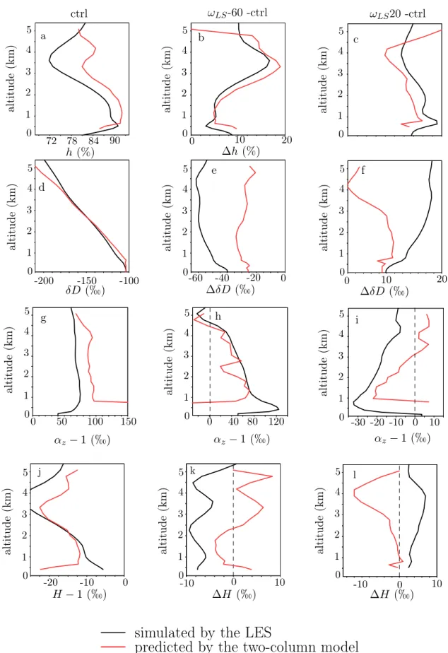
222

when all isotopic exchanges are considered (Figure 3c, green). Rain-vapor vapor diffusive exchanges thus play an

223

important role as well.

224

We note that the δDv difference between the simulations is remarkably constant with altitude (Figure 3a,c),

225

although we expect strong vertical variations in rain evaporation. This is consistent with the important role of the

226

SCL δDvas an initial condition for the full δDvprofile. We also note that more enriched δDvprofiles are associated

227

with a reduced lower-tropospheric steepness αzjust above the SCL, and larger δDv differences between simulations

228

are associated with larger differences in lower-tropospheric αz. This is consistent with the SCL δDv being mainly

229

driven by the steepness αz just above the SCL ([Risi et al., 2020]). Finally, the reduced “vapor amount effect” in

230

“nofrac” leads to a reduced amount effect in the precipitation δD as well (Figure 3c, circles). This shows that the

231

column-integrated water budget ([Lee et al., 2007, Moore et al., 2014]) cannot by itself predict the amount effect,

232

since it depends on the isotopic composition of the advected vapor, which can greatly vary depending on the detalied

233

representation of rain evaporation processes.

234

To summarize, in the total δDvdifference between ωLS−60 and ctrl, there is about one third due to fractionation

235

during evaporation, one third due to rain-vapor diffusive exchanges, and one third that would remain even in absence

236

of any fractionation during evaporation. These tests suggest that hypotheses 2 and/or 3 play a key role in the “vapor

237

amount effect”. In the next sections, we aim at better understanding how rain evaporation impacts δDv profiles.

238

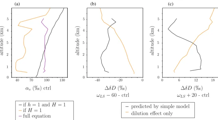
2.5

Vertical profiles binned by moist static energy

239

Previous studies have shown that analyzing variables in isentropic coordinates was a powerful tool to categorize

240

the different convective structures: undiluted updrafts, diluted updrafts, saturated and unsaturated downdrafts,

241

and the environment ([Kuang and Bretherton, 2006, Pauluis and Mrowiec, 2013]). This method also has the

ad-242

vantage of filtering out gravity waves. It has been applied to the analysis of a wide range of convective systems

243

([Mrowiec et al., 2015, Mrowiec et al., 2016, Dauhut et al., 2017, Chen et al., 2018]).

244

Here we use the frozen moist static energy m as a conserved variable because it is conserved during condensation

245

and evaporation of both liquid and ice water ([Muller and Romps, 2018, Hohenegger and Bretherton, 2011]).

246

m = cpd·T + g · z + Lv·qv−Lf·qi

where cpd is the specific heat of dry air, T is temperature, g is gravity, z is altitude, Lv and Lf are the latent

247

heat of vaporization and fusion, and qi is the total ice water content (cloud ice, graupel and snow). At each level,

248

we categorize all grid points into bins of m with a width of 0.4 kJ/kg.

249

The domain-mean frozen moist static energy m decreases from the upper troposphere down to about 5 km, due

250

to the loss of energy by radiative cooling, and then increases down to the surface due to the input of energy by

251

surface fluxes (Figure 4, solid black line). Based on this diagram, we can identify four kinds of air parcels:

−140 −130 −120 −110 −100 −90 −80 −70 −60 −50 1 2 3 4 5 6 7 8 9 −90 −80 −70 −60 −50 −40 −30 −20 −10 0 −360 −300 −240 −180 −120 0 2 4 6 8 10 66 72 78 84 90 0 2 4 6 8 10 0 2 4 6 8 10 0 60 120 180 240 −500 −400 −300 −200 −100 −2 −1 0 1 2 3

(b)

(c)

(d)

(e)

(a)

h (%)

al

ti

tu

d

e

(k

m

)

α

z

−

1 (h)

δD (h)

al

ti

tu

d

e

(k

m

)

al

ti

tu

d

e

(k

m

)

ln(q) ()

ln

(R

)

·

10

00

(

h

)

δD

v

(

h

)

precipitation (mm/d)

δD

p

(

h

)

δD

p

δD

v

ctrl

ω

LS

−

60

ω

LS

20

Figure 2: (a) Water vapor (circles) and precipitation (squares) δDv as a function of precipitation. Vertical distri-bution of relative humidity (b), water vapor δD (c) and αz(e) in ctrl (black), ωLS−60 (red) and ω_LS+ 20 (green). (c) ln(R(z)) · 1000 as a function of ln(q(z)) for different altitudes. In c and e, dashed lines indicate the prediction by Rayleigh distillation. The horizontal lines show the altitude of the melting level.

0 2 4 6 8 10 0 2 4 6 8 10 0 2 4 6 8 10 0 2 4 6 8 10 −360 −300 −240 −180 −120 −50 −60 −40 −30 −20 −10 0 40 80 120 40 60 80 100 20

(b)

(a)

(d)

(c)

al

ti

tu

d

e

(k

m

)

al

ti

tu

d

e

(k

m

)

al

ti

tu

d

e

(k

m

)

al

ti

tu

d

e

(k

m

)

δD (h)

α

_z

−

1 (h)

∆δD (h)

∆α

_z

−

1 (h)

ω

LS

−

60 - ctrl

ω

LS

−

60 - ctrl

ctrl

nodiff

nofrac

Figure 3: (a) Vertical distribution of δDv for ctrl, when fractionation during liquid evaporation is turned on (black) or off (red) and when liquid-vapor equilibration is turned off (green).

(b) Same as (a) for the vertical profiles of αz.

(c) δDv difference between the ωLS−60 and ctrl, with (black) and without (red) fractionation during evaporation and when liquid-vapor equilibration is turned off (green). The circles illustrate the difference in the precipitation δD.

330 340 350 330 340 350 330 340 350 330 340 350 10 8 6 4 2 0 10 8 6 4 2 0 10 8 6 4 2 0 10 8 6 4 2 0 10 8 6 4 2 0 10 8 6 4 2 0 10 8 6 4 2 0 10 8 6 4 2 0 330 340 350 330 340 350 330 340 350 330 340 350 (a) (b) (c) (d) (e) (f) (g) (h)

MSE (kJ/kg)

MSE (kJ/kg)

MSE (kJ/kg)

MSE (kJ/kg)

al

ti

tu

d

e

(k

m

)

al

ti

tu

d

e

(k

m

)

al

ti

tu

d

e

(k

m

)

al

ti

tu

d

e

(k

m

)

al

ti

tu

d

e

(k

m

)

al

ti

tu

d

e

(k

m

)

al

ti

tu

d

e

(k

m

)

al

ti

tu

d

e

(k

m

)

MSE (kJ/kg)

MSE (kJ/kg)

MSE (kJ/kg)

MSE (kJ/kg)

cloud water (g/kg)

precipitation water (g/kg)

dq

v

/dt (g/kg/d)

dq

v

/dt.nb (g/kg/d)

log

10

(nb)

w (m/s)

w.nb.ρ (kg/m

2

/d)

h (%)

Figure 4: Variables binned as a function of frozen moist static energy m and of altitude, for the ctrl simulation: (a) number of samples, (b) vertical velocity anomaly, (c) vertical mass flux (vertical velocity multiplied by the proportion of samples and density), (d) relative humidity, (e) cloud water content mixing ratio (liquid and ice), (f) precipitating water mixing ratio (rain, graupel and snow), (g) evaporation and condensation tendency (positive in case of evaporation, negative in case of condensation), (h) δDv anomaly, (i) (φ − 1) · 1000, where φ = Rev/Rv; it is expressed in h. The solid black line show the domain-mean frozen moist static energy, while the dashed black line shows the frozen moist static energy at saturation.

10 8 6 4 2 0 10 8 6 4 2 0 10 8 6 4 2 0 10 8 6 4 2 0 10 8 6 4 2 0 10 8 6 4 2 0 330 340 350 330 340 350 _{340 350 330} 340 340 350 330 340 (a) (b) (c) (e) (f) (d)

al

ti

tu

d

e

(k

m

)

al

ti

tu

d

e

(k

m

)

al

ti

tu

d

e

(k

m

)

al

ti

tu

d

e

(k

m

)

al

ti

tu

d

e

(k

m

)

al

ti

tu

d

e

(k

m

)

MSE (kJ/kg)

MSE (kJ/kg)

MSE (kJ/kg)

MSE (kJ/kg)

MSE (kJ/kg)

MSE (kJ/kg)

δD

′ v

(h)

δD

′ v

(h)

δD

′ v

(h)

R

ev

/R

v

−

1 (h)

R

ev

/R

v

−

1 (h)

R

ev

/R

v

−

1 (h)

ctrl

ω

LS

−

60

ω

LS

+ 20

Figure 5: (a,d) As for Figure 4 but for (a) δDv anomaly, (d) (φ − 1) · 1000, where φ = Rev/Rv; it is expressed in h_{. (b,e) As for (a,d) but for ωLS}−60. (c,f) As for (a,d) but for ω_LS+ 20.

1. Environment. They correspond to air parcels whose m is close to the domain-mean (solid black). They are the

253

most numerous (Figure 4a). Their vertical velocity is slightly descending (Figure 4b), but because they are

254

very numerous, they account for most of the downward mass flux (Figure 4c). Their relative humidity is close

255

to the domain-mean (Figure 4d), they contain only a small cloud water and rain content and phase changes

256

are very slow (Figure 4e-g). However, because they cover most of the domain, they contribute significantly to

257

the evaporation in the domain-mean (Figure 4h).

258

2. Cloudy updrafts. They correspond to air parcels on the right of the domain-mean m and whose bin-mean

259

vertical velocity is ascending (Figure 4b). If air rose adiabatically from the SCL, they would conserve their

260

m and they would be located completely on the right of the diagram. In practice, m decrease because the

261

environment air is progressively entrained into ascending parcels. In the diagrams, parcels are more diluted

262

when they are closed to the domain-mean, and less diluted when they are more to the right. In spite of their

263

dilution with the environment, their humidity is at saturation ( (Figure 4d). They contain a lot of cloud and

264

precipitating water, and vapor undergoes condensation (Figure 4e-g).

265

3. Cloudy downdrafts. They correspond to air parcels on the right of the domain-mean m and whose bin-mean

266

vertical velocity is descending (Figure 4b). They are more diluted than cloudy updrafts. Their humidity is

267

below saturation (Figure 4d). They contain cloud and precipitating water, but these hydrometeor undergo

268

evaporation (Figure 4e-g). Located around the cloudy updrafts in the real space, they mainly correspond to

269

subsiding shells ([Glenn and Krueger, 2014]).

270

4. Precipitating downdrafts. They correspond air parcels on the bottom-left of the diagrams, with lower m

271

relative to the domain-mean. They are among the most strongly descending air parcels (Figure 4b), but

272

since they are scarce (Figure 4b), they contribute little to the total descending mass flux (Figure 4c). They

273

are very dry, with no cloud water, but with precipitating water (Figure 4d-f). We interpret these parcels

274

as unsaturated, precipitating downdrafts. Strong evaporation of rain occur in these downdrafts (Figure 4g),

275

but because they cover only a small fraction of the domain, they contribute little to the evaporation in the

276

domain-mean (Figure 4h).

277

The isotopic composition of water vapor is the strongest in the least diluted updrafts, and the most depleted in the

278

precipitating downdrafts (Figure 5a). To assess the effect of phase changes, we plot φ = Rev/Rv, where Rev is the

279

ratio of the water vapor tendency associated with phase changes (evaporation in downdrafts and in the environment,

280

or condensation in cloudy updrafts) and Rv is the isotopic ratio of the water vapor. In cloudy updrafts, φ − 1 is

281

about 100h in the lower troposphere and increases with height (Figure 5b). This corresponds roughly to equilibrium

282

fractionation during condensation. In cloudy downdrafts, φ − 1 is also about 100h. This means that cloud droplets

283

evaporate totally without fractionation. In contrast, in precipitating downdrafts, φ − 1 is much lower. It is around

284

30h below 1 km. The fact that φ − 1 is positive is consistent with the fact that rain evaporation in the SCL acts

285

to slightly enrich the water vapor ([Risi et al., 2020]). In contrast, between 2 and 3 km, φ − 1 is around -100h: at

286

these levels, rain evaporation acts to deplete the water vapor, consistent with [Worden et al., 2007].

287

These diagrams look qualitatively similar for the other simulations. One noticeable difference is that in ωLS−60,

288

the δDv contrast between the environment and the cloudy regions is larger (Figure 5b). This may be associated

289

with the more depleted evaporation of the rain in precipitating downdrafts, and even of cloud droplets in cloudy

290

downdrafts (Figure 5e). Conversely, in ωLS+ 20, the δDv contrast between the environment and the cloudy regions

291

is larger (Figure 5c). To quantitatively compare the different simulations, now we plot vertical profiles of variables

292

in average over cloudy regions and over the environment.

293

2.6

Vertical profiles for cloudy regions and for the environment

294

Here we chose to define cloudy regions as all parcels with a cloud (liquid or ice) water content greater than 10−6_g/kg

295

(e.g. [Thayer-Calder and Randall, 2015]). In this loose definition, “cloudy regions” correspond to both cloudy

296

updrafts and downdrafts, while the “environment” includes both the environment and precipitating downdrafts.

297

Including the cloudy downdrafts into the cloudy regions is justified by the fact that a significant portion of the

298

water condensed in cloudy updrafts subsequently evaporate in these cloudy downdrafts, without directly affecting

299

the environment. Our results below are not crucially sensitive to the definition of the distinction between cloudy

300

regions and the environment, provided that the definition of cloudy regions is not too restrictive (Text S1).

301

Cloudy regions cover only a few percent of the domain (Figure 6a). The fraction of water condensed in cloudy

302

regions that evaporates into the environment, estimated as fev= −(dq/dt)env/(dq/dt)cloud, where (dq/dt)env and

303

(dq/dt)cloud are the humidity tendencies associated with phase changes in average in the environment and in the

0 2 4 6 1 3 5 0 2 4 6 1 3 5 0 2 4 6 1 3 5 0 1 2 3 4 5 6 30 40 50 60 70 80 90 0 20 40 60 80 100 120 (a) (b) (c)

f

ev

(%)

φ − 1 (h)

ctrl ωLS−60 ωLS+ 20

cloud fraction (%)

al

ti

tu

d

e

(k

m

)

al

ti

tu

d

e

(k

m

)

al

ti

tu

d

e

(k

m

)

Figure 6: (a) fraction of the domain-area covered by cloudy regions. (b) Fraction of the water condensed in cloudy regions that evaporates into the environment, fev. (c) (φ − 1) · 1000 (solid) and (αeq−1) · 1000 (dashed), where φ = Rev/Reand αeq is the equilibrium fractionation coefficient. Both are expressed in h. The black, red and green lines are for ctr, ωLS−60 and ωLS+ 20 respectively.

cloudy region respectively, varies between 30% and 90%, depending on altitude (Figure 6b). It is smaller in ωLS−60

305

and than in ctrl, because the environment is moister.

306

Figure 6c plots φ = Rev/Re, where Rev = (dqHDO/dt)env/(dq/dt)env, (dqHDO/dt)env is the HDO tendency

307

associated with phase changes in the environment and Reis the isotopic ratio in the environment. In ctrl , φ > 1:

308

the evaporation has an enriching effect on the environment. Yet, φ < αeq: the evaporation is not as enriching

309

as if there was total evaporation of condensate. In ωLS−60, φ is smaller than in ctrl: rain evaporation has a

310

weaker enriching effect. At 4.5 km, near the melting level, there is a small layer where φ < 1 : at this level, the

311

rain evaporation has a depleting effect on the water vapor. The overall enriching effect of evaporation contradicts

312

hypothesis 2, but the weaker enriching effect in ωLS−60 than in ctrl supports hypothesis 3. Conversely, φ is larger

313

in ωLS+ 20.

314

2.7

What controls the isotopic composition of the rain evaporation flux?

315

Why is φ smaller in ωLS−60 and higher in ωLS+ 20 than in ctrl? It could be because rain-vapor exchanges in a

316

moister environment leads the evaporation to have a more depleting effect ([Lawrence et al., 2004, Risi et al., 2008]),

317

or because rain evaporation is more depleted when the evaporated fraction is small ([Risi et al., 2008, Tremoy et al., 2014]),

318

or because the rain itself is more depleted. We aim here at quantifying these different effects.

319

Figure 7a plots the vertical profiles of rain δD (solid). Below the melting level, the rain is very close to isotopic

320

equilibrium with the vapor (dashed). Above the melting level, the rain is more enriched than if in equilibrium due

321

to rain lofting. Near the melting level for simulation ωLS−60, the rain is anomalously depleted. This is due to

322

snow melt. Since the snow forms higher in altitude, it is more depleted than the rain. It thus imprints its depleted

323

signature on the rain when melting. In ωLS−60, the moist middle troposphere prevents most of the snow from

324

sublimating: 24% of the precipitation is made of snow at the melting level. The rain is thus strongly depleted by

325

snow melt. In contrast, in ctrl and ωLS+ 20, the drier middle troposphere favors snow sublimation: only 8% and

326

3% of the precipitation is made of snow at the melting level respectively.

327

The quick equilibration between the rain and vapor motivates us to use a simple equation in which some mass

328

ql0 of rain, with isotopic ratio Rl0, partially evaporates and isotopically equilibrates with some mass qv0 of vapor,

329

with isotopic ratio Rv0. As explained in text S2, if ql0≫qv0, we get:

φ = λ

αeq−fev·(αeq−1)

(2) where φ = Rev/Rv0, λ = Rl0/Rv0, Rev is the isotopic ratio of the rain evaporation flux, αeq is the equilibrium

331

fractionation coefficient and fev is the fraction of the rain that evaporates. Equation 2 tells us that the rain

332

evaporation is more depleted as the rain is more depleted relative to the vapor (quantified by λ) and as the

333

evaporated fraction fev is smaller. This simple equation (Figure 7b, red) is able to approximate the simulated

334

values of φ (black) for the ctrl simulation and is able to capture the smaller and larger values of φ for ωLS−60 and

335

ωLS+ 20 respectively (Figure 7c-d).

336

We find that below the melting level, φ is smaller in ωLS−60 than in ctrl mainly because fevis smaller (Figure

337

7c, green). Near the melting level, φ is smaller in ωLS−60 than in ctrl both because fev is smaller and because λ

338

is smaller, i.e. the rain is more depleted due to snow melt. In ωLS+ 20 , the effect of fev dominates at all levels.

339

2.8

Summary

340

To summarize, the previous sections suggest that rain evaporation in the lower troposphere is a key ingredient of

341

the vapor amount effect. The isotopic composition of the rain evaporation flux mainly depends on the evaporated

342

fraction of the rain (consistent with [Risi et al., 2008, Tremoy et al., 2014]). Near the melting level in regimes of

343

large-scale ascent, it is also impacted by snow melt. We hypothesize that the isotopic effect of rain evaporation

344

propagates downward down to the SCL. To test this hypothesis and to understand the underlying mechanisms, in

345

the next section we develop a simple two-column model.

346

3

A simple two-column model to quantify the relative contributions of

347

different processes

348

The previous section and previous studies provide a guide for developing our simple interpretative framework. First,

349

the model needs to represent the effect of rain evaporation, highlighted as a key process in the previous section.

350

Second, alternative hypotheses for the “vapor amount effect” have involve mixing between the subsident environment

351

and detrained water ([Bailey et al., 2017], hypothesis 4). These processes also need to be represented in our model.

352

Third, the steepness of the q − δDv relationship must be a key ingredient, since it drives δDv in the SCL and thus

353

δDv everywhere. Finally, the previous section has relied on the distinction between the environment and cloudy

354

regions. Keeping this distinction, we develop a two-column model.

355

3.1

Model equations and numerical application to LES outputs

356

3.1.1 Balance equations

357

This model is inspired by the two-column model used to predict tropospheric relative humidity in [Romps, 2014]

358

and δD profiles in [Duan et al., 2018]. The first column represents the cloudy regions, including cloudy updrafts and

359

downdrafts, as a bulk entraining plume. The second column represents the subsident environment and precipitating

360

downdrafts (Figure 8).

361

The mass balance for the air in the cloudy regions writes:

362

dM

dz = M · (ǫ − δ) (3)

where M is the bulk mass flux in the cloudy regions (positive upward), ǫ and δ are the fractional entrainment

363

and detrainment rates.

364

We assume that the specific humidity in the cloudy regions is at saturation, and call it qs. The water balance

365

in the cloudy regions writes:

366

d (M qs)

dz = ǫ · M · qe−δ · M · qs−c (4)

where c is the condensation rate and qe is the specific humidity in the environment. The terms on the right

367

hand side represent the water input by entrainment of environment air, the water loss by detrainment of cloudy air,

368

and the water loss by condensation respectively. We assume that all the condensed water is immediately lost by the

(c)

_(d)

−90

−60

−30

0

−20

0

20

40

5

4

3

2

1

0

5

4

3

2

1

0

−20

−60

−100

−140

−180

30

60

90

120

(a)

(b)

5

4

3

2

1

0

5

4

3

2

1

0

LES

Eq

LES

Eq

f

ev

only

λ only

al

ti

tu

d

e

(k

m

)

al

ti

tu

d

e

(k

m

)

∆φ (h) ωLS20-ctrl

∆φ (h) ωLS

−

60-ctrl

φ − 1 (h) ctrl

δD (h)

al

ti

tu

d

e

(k

m

)

al

ti

tu

d

e

(k

m

)

ctrl

ω

LS

−

60

ω

LS

20

rain

liquid in eq.

with vapor

snow

Figure 7: (a) δD profile for rain water (solid) and snow (dotted) falling in the environment. The liquid that would be in equilibrium with the vapor in the environment is shown in dashed. (b) Profile of φ = Rev/Resimulated by the ctrl simulation (black, same as in Figure 6c black) and predicted by equation 2 (red). (c) Difference of φ between ωLS−60 and ctrl simulated by the LES (black), predicted by the equation 2 (red), predicted by equation 2 if only

downdrafts and unsaturated environment cloudy updrafts and downdrafts −M qe = h · qs Re= H · Rs large-scale ascent η · M Rs= Rs0·e−(αs−1)·γ·(z−z0) qs= qs0·e−γ·(z−z0) M µ · M · qs·γ evaporation fev·µ φ · Re condensation δ ǫ αeq ·R_s

Figure 8: Schematic view of the simple two-column model, and definition of the main variables.

cloudy regions to the environment, and evaporation of this lost water can occur in the sub-saturated environment

370

only (as in [Romps, 2014]).

371

We assume that mass is conserved within the domain, so that the flux in the environment is −M . The

large-372

scale ascent, when present, is taken into account through a humidity tendency, consistent with the LES set-up. We

373

assume that the large-scale humidity tendency applies to the environment only, which is a first-order approximation

374

justified by the small fraction of the domain that is covered by cloudy updrafts (less than 10%). The water balance

375

in the environment writes:

376

d (−M qe)

dz = −ǫ · M · qe+ δ · M · qs+ fev·c − η · M · ∂qe

∂z (5)

where fev is the fraction of the cloud or precipitating water that evaporates in the environment, η = MLS/M

377

and MLSis the domain-mean large-scale mass flux. The terms on the right hand side represents the water loss by

378

entrainment into cloudy regions, water input by the detrainment of cloudy air, partial evaporation of condensed

379

water and water input by large-scale vertical advection.

380

Regarding water isotopes, we assume that the cloud water removed by condensation is in isotopic equilibrium

381

with the cloudy region water vapor. The isotopic balance in the cloudy regions thus writes:

382

d (M qs·Rs)

dz = ǫ · M · qe·Re−δ · M · qs·Rs−c · αeq·Rs (6) where αeqis the equilibrium fractionation coefficient, Rsis the isotopic ratio in the cloudy regions and Reis the

383

isotopic ratio in the environment.

384

The isotopic balance in the environment writes:

385

d (−M qe·R_e)

dz = −ǫ · M · qe·Re+ δ · M · qs·Rs+ fev·c · φ · Re−η · M ·

∂ (qeRe)

∂z (7)

where recall that φ = Rev/Reand Rev is the ratio of the precipitation evaporation flux.

386

3.1.2 Other simplifying assumptions and differential equations

387

To simplify the equations, as in [Romps, 2014] we assume that qs is an exponential function of altitude:

388

where γ is a lapse rate in m−1_{calculated as d ln(qs)/dz.}

389

For isotopes, we assume that the Rsis a power function of qs, consistent with a Rayleigh distillation:

390

Rs= Rs(z0) (qs/qs0)as−1

Coefficient αs represents the steepness of the q − δDv gradient in cloudy regions and remains to be estimated.

391

As in [Duan et al., 2018], Rsis thus an exponential function of altitude:

392 Rs= Rs(z0) · e−(αs−1)·γ·(z−z0) (9) We set: 393 qe= h · qs Re= H · Rs

Combining equation 5 with equations 3 and 8, we get the following differential equation for h:

394 ∂h ∂z = h · γ − δ 1 − η(1 − h) − fev·µ · γ 1 − η (10)

where µ = c/(M · qs·γ) represents the ratio of actual condensation (c) relative to the condensation if the ascent

395

was adiabatic (M · qs·γ). Similarly, combining equations 7 with equations 5 and 9, we get the following differential

396 equation for H: 397 ∂H ∂z = H · γ · (αs−1) − δ h · (1 − η)·(1 − H) − fev·µ · γ h · (1 − η)·H · (φ − 1) (11)

We now have two equations with four unknowns: h, H, µ and αs. The condensation efficiency µ can be deduced

398

from equations 4:

399

µ = 1 − ǫ

γ·(1 − h) (12)

This equation, similar to one in [Romps, 2014], reflects the fact that condensation efficiency decreases when

400

entrainment ǫ increases and when the entrained air is drier. If ǫ = 0 or h = 1, then µ = 1.

401

Similarly, the q − δDv steepness αs in cloudy air can be deduced from equation 6:

402

αs−1 = µ · (αeq−1) + ǫ

γ·h · (1 − H) (13)

This equation tells us that two effects control the steepness of the q − δDv gradient. First, there is a “dilution

403

effect”: if dry air is entrained, then the condensation efficiency µ decreases. This reduces αs compared to αeq,

404

i.e. compared to what we would expect from Rayleigh distillation. Second, there is an “isotopic contrast effect”: if

405

depleted water vapor is entrained (H < 1) is entrained, then αsbecomes steeper. This is how a depleting effect of

406

rain evaporation can translate into a larger steepness, and eventually more depleted SCL.

407

3.1.3 Numerical solutions

408

To get analytical solutions for h and H, [Romps, 2014] and [Duan et al., 2018] assume that h ·∂qs

∂z ≫qs· ∂h ∂z and 409 that H ·∂Rs ∂z ≫Rs· ∂H

∂z. This allows them to calculate h and H as the solution of a simple linear equation and of

410

a second order polynomial respectively. However, there are two issues with these solutions. First, although these

411

solutions behave reasonably for h ( [Romps, 2014]), they become very noisy, unstable or unrealistic for values of

412

ǫ, δ and fev that are diagnosed from LES outputs. This is because there is a powerful positive feedback between

413

αs and H: as H decreases, more depleted vapor is entrained in updrafts which increases the steepness αs; in turn,

414

the stronger steepness αsmakes the subsidence more efficient at depleting the environment, further decreasing H.

415

[Duan et al., 2018] circumvented this problem by assuming ǫ and δ that are constant with altitude and equal to

416

each other, but it is at the cost of artificially reducing freedom for the solutions. Second, our hypothesis is that rain

417

evaporation near the melting level affects the isotopic profiles down to the SCL. We thus want each altitude to feel

418

the memory of processes at higher altitudes. The term with ∂H_∂z is thus a key ingredient in our framework.

419

Therefore, we choose to numerically solve the differential equations 10 and 11. We start from an altitude of

420

5 km with h = 0.8 and H − 1 = −10h. We do not start above 5 km because entrainment is more difficult to

diagnosed above the melting level (section 3.1.4). We integrate equations 10 and 11 down to the SCL top around

422

500 m. The resulting h profile is a function of the profiles of 5 input parameters: γ, ǫ, δ, fev and η . The H profile

423

is a function of 7 input parameters: γ, ǫ, δ, fev, η, αeq and φ. These input parameters are all diagnosed from the

424

LES simulations as detailed below. In each LES level, the input parameters are assumed constant and equations

425

10 and 11 are integrated within each layer over 50 sub-layers.

426

3.1.4 Diagnosed input parameters

427

Parameters fev, αeq and φ were already plotted in Figure 6 and discussed in section 2.6. Parameter γ is calculated

428

from domain-mean profiles. It is steeper in ctrl than in ω − 60 because of the steeper temperature gradient resulting

429

from the drier air (Figure 9a). Parameter η = MLS/M is calculated from the net upward mass flux in cloudy

430

regions M (Figure 9b), which is calculated as the average vertical velocity in cloudy regions multiplied by the area

431

fraction of the cloudy region. Entrainment ǫ is diagnosed by using the conservation of the frozen moist static energy

432

(e.g. [Hohenegger and Bretherton, 2011, Del Genio and Wu, 2010]):

433

∂ms

dz = ǫ · (me−ms)

where msand me are the frozen moist static energy in the convective region and the environment respectively.

434

The application of this equation is limited to the lower troposphere. Above the melting level, we would need to

435

account for the precipitation of ice ([Pauluis and Mrowiec, 2013]) and for the lofting of rain. Therefore, we arbitrarily

436

set ǫ = 0.5 km−1_{above the melting level. Entrainment is maximal in the sub-cloud layer, and decreases exponentially}

437

with height (Figure 9c), consistent with previous studies ([Del Genio and Wu, 2010, De Rooy et al., 2013]).

438

Finally, detrainment δ is deduced from ǫ and M using equation 3. Detrainment shows the typical trimodal

439

distribution ([Johnson et al., 1999]) (Figure 9d), with a first maximum just above the SCL top corresponding to

440

the detrainment of shallow convection, a second maximum near the melting level near 4.5 km corresponding to the

441

detrainment of congestus convection, and a third maximum in the upper troposphere corresponding to the deep

442

convection (not shown in 9d).

443

3.1.5 Closure in the sub-cloud layer

444

To calculate the full δD profiles, we need as initial condition the isotopic ratio in the SCL. With this aim, we use a

445

simplified version if the sub-cloud layer model of [Risi et al., 2020]. We assume that water enters the SCL through

446

surface evaporation and through downdrafts at the SCL top, and exits the SCL through updrafts at the SCL top.

447

We neglect large-scale forcing and rain evaporation, since they have a small impact in the SCL ([Risi et al., 2020]).

448

The air flux of updrafts equals that of downdrafts. We define ru= qu/q1 and rd = qd/q1, where q1 is the mixing

449

ratio in the SCL and qu and qd are the mixing ratios in updrafts and downdrafts at the SCL top. We assume

450

that the water vapor is more enriched as the air is moister, following a logarithmic function: Ru = R1·rαuu−1

451

and Rd = R1·rdαd−1 where Ru and Rd are isotopic ratios in updrafts and downdrafts, and αu and αd are q − δD

452

steepness for updrafts and downdrafts. Water and isotopic budgets yield:

453 R1= Roce/αeq(SST ) h1+ αK·(1 − h1) · rαu u −rdαd ru_−rd (14) where Roce is the isotopic ratio at the ocean surface, αeq(SST ) is the equilibrium fractionation coefficient

454

at the sea surface temperature, αK is kinetic fractionation coefficient ([Merlivat and Jouzel, 1979]) and h1 is the

455

relative humidity normalized at the SST and accounting for ocean salinity: h1 = q1/qsurfsat (SST ), q surf

sat (SST ) =

456

0.98 · qsat(SST ) and qsat is the humidity saturation as a function of temperature at the sea level pressure. We

457

assume δDoce= 0h and h1 is diagnosed from the LES.

458

For ru and rd, we use values for the ctrl simulation, because small changes in ru and rd across simulations

459

have only a marginal impact on R1 ([Risi et al., 2020]). Following [Risi et al., 2020], we set ru−1=1.44% and

460

rd−1=-0.38%. For αu and αd, [Risi et al., 2020] had shown that they scale with αz values just above the SCL

461

top, but with larger values especially for simulations with large-scale ascent. We use an empirically-fitting function:

462

αu = αd= 1 + 100 · (fαz−1)3, where fα_z= 1 + ln(R(zSCT)/R(zSCT+1 km))

ln(q(zSCT)/d(zSCT+1 km)) where zSCT is the SCL top. 463

Finally, since the updraft region covers only a very small fraction of the domain, we assume that Re(zSCT) ≃ R1.

464

The procedure to calculate the full δDv profiles is as follows:

465

1. vertical profiles for h, H and αs are calculated through a downward integration of equations 10-13 following

466

3.1.3.

(a)

(b)

(c)

(d)

0

1

2

4

5

5

al

ti

tu

d

e

(k

m

)

6

0

1

2

4

5

5

al

ti

tu

d

e

(k

m

)

6

0

1

2

4

5

5

al

ti

tu

d

e

(k

m

)

6

0

1

2

4

5

5

al

ti

tu

d

e

(k

m

)

6

-40

-20

0

20

40

0

0.6

1.2

1.8

2.4

η (%)

δ (km

−1

)

0.18 0.24

0.3

0.36 0.42 0.48

γ (km

−1

)

0

2

4

6

8

10

ǫ (km

−1

)

ctrl

ω

LS

−

60

ω

LS

20

Figure 9: Input parameters for the simple model, for ctrl (black), ωLS−60 (red) and ω_LS+20 (green). (a) saturation specific humidity lapse rate γ; (b) ratio of large-scale vertical mass flux over the convective cloud mass flux; (c) entrainment rate; (d) detrainment rate.

2. The vertical profile for a normalized version of Rs, Rs,norm that satisfies Rs,norm(zSCT) = 1, is calculated

468

based on the αsprofile through an upward integration.

469

3. The vertical profile for a normalized version of Re, Re,norm, is calculated as Re,norm= Rs,norm·H.

470

4. From the Re,normprofile, fαz is estimated.

471

5. From h1 and fαz, R1 is estimated.

472

6. The full Reprofile can finally be calculated so that Re(zSCT) ≃ R1: Re= Re,norm·R1/H(zSCT).

473

3.1.6 Evaluation of the two-column model

474

The two-column model successfully captures the order of magnitude and the shape of the vertical profile of relative

475

humidity for the ctrl simulation (Figure 10a), as well as the moister troposphere in ωLS−60 and the drier troposphere

476

in ωLS+ 20 (Figure 10b-c).

477

It successfully captures the vertical profile of δDv (Figure 10b) and the more depleted troposphere in ωLS−60

478

but underestimate the δDvdifference by about half (Figure 10e). It also captures the more enriched troposphere in

479

ωLS+ 20 but again underestimate the δDvdifference especially in the middle troposphere (Figure 10f). Similarly, it

480

approximately captures the steepness αz and the sign of the αz differences across simulations, but underestimates

481

the αz differences (Figure 10g-i).

482

These mismatches are caused by mismatches in the estimate of the relative enrichment of the environment

483

relative to the updrafts H. Although it is reasonably well predicted for the ctrl simulation (Figure 10c), the model

484

fails to simulate the smaller H for ωLS−60 in the middle troposphere and the larger H for ωLS+ 20 almost

485

everywhere. The two-column model overestimates the impact of η and predicts a behavior for H that is too similar

486

to that of h. We could not find the exact reason for this shortcoming, but we have to acknowledge that the

487

two-column model hides many horizontal heterogeneities. We will have to keep this shortcoming in mind when

488

interpreting the results.

489

3.2

Decomposition of relative humidity and

δD variations

490

To estimate the impact of the different input parameters on the relative humidity profile h, we modify them one by

491

one from the ctrl simulation to the ωLS−60 and from the ctrl simulation to ωLS+ 20 simulations.

492

3.2.1 Decomposition of relative humidity

493

The moister troposphere in ωLS−60 is mainly due to the larger η, i.e. the direct moistening effect of large-scale

494

ascent (Figure 11a). The thermodynamic structure, entrainment, detrainment and rain evaporation have a much

495

smaller effect. Similarly, The drier troposphere in ωLS+ 20 is mainly due to the more negative η, i.e. the direct

496

drying effect of large-scale descent (Figure 11b).

497

Note that the direct effect of η on environment relative humidity may be an artifact of the way the

large-498

scale forcing is prescribed in our LES. The large-scale circulation is accounted for through tendencies in humidity,

499

temperature and isotopes that are horizontally homogeneous. Therefore, since the environment covers most of the

500

domain, most of the large-scale ascent or descent is felt in the environment. In reality, in case of large-scale ascent

501

for example, we expect the environment to keep the same subsidence rate, corresponding to radiative subsidence.

502

Rather, we expect the large-scale ascent to be absorbed by the larger cloud fraction ([Emanuel et al., 1994]). In our

503

interpretative framework, this would be equivalent to adding the large-scale in the cloudy column rather than in

504

the environment. This would increase the condensation efficiency µ, and would eventually moisten the environment

505

through rain evaporation, but less than if the large-scale ascent was homogeneous (Text S3). We have to keep this

506

in mind if trying to connect the sensitivity of h to large-scale circulation in our LES and in reality.

507

3.2.2 Dilution effect onδD

508

A first effect impacting δDv profiles is the dilution by entrainment (section 3.1.2). In the absence of entrainment

509

(ǫ = 0), the steepness in the updraft column would be αs= αeq (Figure 12a, black). Because dry air is entrained,

510

the condensation rate is reduced by the factor µ following equation 12. According to equation 13, this reduces the

511

steepness (Figure 12a, green). This effect of entrainment can be understood as a mixing process: as the air rises and

512

condensation proceeds, the remaining air is mixed with dry air from entrainment and with droplets that evaporate.

513

Consistent with the convex shape of the mixing lines, this leads to a reduction of the q − δD steepness (Figure 1).

simulated by the LES

predicted by the two-column model

0 1 2 4 5 3

al

ti

tu

d

e

(k

m

)

0 1 2 4 5 3

al

ti

tu

d

e

(k

m

)

20 10 0

∆h (%)

-60 -40 -20 0 0 1 2 4 5 3

al

ti

tu

d

e

(k

m

)

0 1 2 4 5 3

al

ti

tu

d

e

(k

m

)

-10 0 10 0 1 2 4 5 3

al

ti

tu

d

e

(k

m

)

72 78 84 90 0 1 2 4 5 3

al

ti

tu

d

e

(k

m

)

0 1 2 4 5 3

al

ti

tu

d

e

(k

m

)

-20 -10 0 0 1 2 4 5 3

al

ti

tu

d

e

(k

m

)

-10 0 10 0 1 2 4 5 3

al

ti

tu

d

e

(k

m

)

0 1 2 4 5 3

al

ti

tu

d

e

(k

m

)

20 10 0 0 1 2 4 5 3

al

ti

tu

d

e

(k

m

)

ω

LS

-60 -ctrl

∆δD (h)

b

e

α

z

−

1 (h)

∆H (h)

0 40 80 120 a 0 1 2 4 5 3

al

ti

tu

d

e

(k

m

)

ctrl

δD (h)

h (%)

d

-200 -150 -100

α

z

−

1 (h)

H − 1 (h)

0 50 100 150

g

h

-30 -20 -10 0 10

∆H (h)

ω

LS

20 -ctrl

∆δD (h)

c

f

α

z

−

1 (h)

i

j k _l

Figure 10: (a) Relative humidity h simulated by the LES (black) and predicted by the two-column model (red) for the ctrl simulation. (b) Same as (a) but for the difference between ωLS−60 and ctrl. (c) Same as (b) but for the difference between ωLS+ 20 and ctrl. (d-f) Same as (a-c) but for the water vapor δD. (g-i) Same as (a-c) but for the steepness αz. (j-l) Same as (a-c) but for the relative enrichment of the environment relative to the updrafts H.