HAL Id: hal-00419212
https://hal.archives-ouvertes.fr/hal-00419212v2
Preprint submitted on 1 Oct 2009
HAL is a multi-disciplinary open access
archive for the deposit and dissemination of
sci-entific research documents, whether they are
pub-lished or not. The documents may come from
teaching and research institutions in France or
abroad, or from public or private research centers.
L’archive ouverte pluridisciplinaire HAL, est
destinée au dépôt et à la diffusion de documents
scientifiques de niveau recherche, publiés ou non,
émanant des établissements d’enseignement et de
recherche français ou étrangers, des laboratoires
publics ou privés.
Damped and sub-damped Lyman-α absorbers in z > 4
QSOs
Rodney Guimaraes, Patrick Petitjean, Reinaldo de Carvalho, George
Djorgovski, Pasquier Noterdaeme, Sandra Castro, Paulo Poppe, Ali Aghaee
To cite this version:
Rodney Guimaraes, Patrick Petitjean, Reinaldo de Carvalho, George Djorgovski, Pasquier
Noter-daeme, et al.. Damped and sub-damped Lyman-α absorbers in z > 4 QSOs. 2009. �hal-00419212v2�
Astronomy & Astrophysicsmanuscript no. dla˙13.hyper7479 October 1, 2009 (DOI: will be inserted by hand later)
Damped and sub-damped Lyman-
α
absorbers in z
>
4 QSOs
⋆
R. Guimar˜aes
1, P. Petitjean
2, R. R. de Carvalho
3, S.G. Djorgovski
4, P. Noterdaeme
5, S. Castro
6, P. C. da R. Poppe
1,
and A. Aghaee
7,81 Universidade Estadual de Feira de Santana - Av. Transnordestina, s/n, 40036-900, Feira de Santana, BA - Brasil 2 UPMC Paris 6, Institut d’Astrophysique de Paris, CNRS, 98bis Boulevard Arago - 75014 Paris, FRANCE
3 Instituto Nacional de Pesquisas Espaciais - INPE, Av. dos Astronautas, 1758, 12227-010, S. J. dos Campos, SP - Brasil 4 California Institute of Technology, MS 105-24, Pasadena, CA 91125
5 Inter-University Centre for Astonomy and Astrophysics, Post Bag 4, Ganeshkhind, Pune 411 007, India 6 Europeen Southern Observatory, Karl-Schwarzschild Strasse, 2, Garching, Germany
7 Department of Physics, University of Sistan and Baluchestan, 98135 Zahedan, Iran
8 School of Astronomy and Astrophysics, Institute for Research in Fundamental Sciences (IPM), P.O.BOX 193595-5531,
Tehran, Iran
Received 17/12/2008; accepted 07/09/2009
Abstract. We present the results of a survey for damped (DLA, log N(H i) > 20.3) and sub-damped Lyman-α systems (19.5 < log N(H i) < 20.3) at z > 2.55 along the lines-of-sight to 77 quasars with emission redshifts in the range 4 < zem<6.3.
Intermediate resolution (R ∼ 4300) spectra have been obtained with the Echellette Spectrograph and Imager (ESI) mounted on the Keck telescope. A total of 100 systems with log N(H i) > 19.5 are detected of which 40 systems are damped Lyman-α systems for an absorption length of ∆X = 378. About half of the lines of sight of this homogeneous survey have never been investigated for DLAs. We study the evolution with redshift of the cosmological density of the neutral gas and find, consistently with previous studies at similar resolution, that ΩDLA,HIdecreases at z > 3.5. The overall cosmological evolution of ΩHIshows a peak around this redshift. The H i column density distribution for log N(H i) ≥ 20.3 is fitted, consistently with previous surveys, with a single power-law of index α ∼ -1.8±0.25. This power-law overpredicts data at the high-end and a second, much steeper, power-law (or a gamma function) is needed. There is a flattening of the function at lower H i column densities with an index of
α ∼ −1.4 for the column density range log N(H i) = 19.5−21. The fraction of H i mass in sub-DLAs is of the order of 30%. The
H i column density distribution does not evolve strongly from z ∼ 2.5 to z ∼ 4.5.
Key words.galaxies: evolution, galaxies: formation, quasars: absorption lines , Intergalactic Medium , cosmology: observa-tions
1. Introduction
The amount of neutral gas in the Universe is an important ingredient of galaxy formation scenarios because the neutral phase of the intergalactic medium is the reservoir for star-formation activity in the densest places of the universe where galaxies are to be formed. It is therefore very important to make a census of the mass in this phase and to determine its cosmo-logical evolution (see e.g. P´eroux et al. 2001).
The gas with highest H i column density is detected through damped Lyman-α absorptions in the spectra of remote quasars. Although damped wings are seen for column densities of the Send offprint requests to: R. Guimar˜aes, e-mail:
rguimara@eso.org
⋆ The observations reported here were obtained with the W. M.
Keck Observatory, which is operated by the California Association for Research in Astronomy, a scientific partnership among the California Institute of Technology, the University of California, and the National Aeronautics and Space Administration.
order of log N(H i) ∼ 18, the neutral phase corresponds to log N(H i) ≥ 19.5 (Viegas 1995). The column density defining the so-called damped Lyman-α (DLA) systems has been taken to be log N(H i) ≥ 20.3 because this corresponds to the criti-cal mass surface density limit for star formation (Wolfe et al. 1986) but also because the equivalent width of the correspond-ing absorption is appropriate for a search of these systems in low resolution spectra. Therefore several definitions have been introduced. ΩDLAg is the mass density of baryons in DLA sys-tems, defined arbitrarily as systems with log N(H i) ≥ 20.3. ΩHI
g
is the mass density of neutral hydrogen in all systems : DLAs, Lyman limit systems (LLS) and the Lyman-α forest. The mass density of H i in the Lyman-α forest is negligible because the slope of the H i column density distribution is larger than −2 (∼ −1.5; the gas is highly ionized). It is more difficult to es-timate the contribution of LLS as the column density of these systems is very difficult to derive directly because the Lyman-α line lies in the logarithmic regime of the curve of growth.
However, ΩHI
g is not easily related to physical quantities as
the LLS with log N < 19.5 are at least partly ionized when the ones with log N > 19.5 are not (see e.g. Meiring et al. 2008). On the contrary, as emphasized by Prochaska et al. (2005), here-after PHW05, the mass density of the neutral phase, Ωneut
g , is
a good indicator of the mass available for star-formation and should be prefered instead. Note that Ωneut
g is not equal to ΩDLAg .
The column density limit at which the gas is mostly neutral can-not be defined precisely but should lie between log N(H i) = 19 and 19.5. In any case, a conservative position is to consider that all systems above 19.5 are neutral.
Whether or not the mass of the neutral gas in the systems with 19.5 < log N(H i) < 20.3 (the so-called sub-DLAs or super-LLS) is negligible has been the source of intense discus-sions in recent years. Note that these discusdiscus-sions are related to the mass in theneutralphase only. Indeed, it is known for long (e.g. Petitjean et al. 1993) that thetotalmass associated with the Lyman limit systems is larger than that of DLAs. Indeed the gas in the LLS phase is mostly ionized and located in extended halos whereas DLAs are located in dense and compact regions. P´eroux et al. (2003), hereafter PMSI03, have been the first to consider the sub-DLAs as an important reservoir of neutral gas. They claim that at z > 3.5, DLAs could contain only 50% of the neutral gas, the rest being to be found in sub-DLAs. When correcting for this, they find that the comoving mass density shows no evidence for a decrease above z = 2. PHW05 ques-tionned this estimate. They use the Sloan Digital Sky Survey to measure the mass density of predominantly neutral gas Ωneutg . They find that DLAs contribute >80% of Ωneutg at all redshift.
Uncertainties are very large however and the same authors es-timate that the systems with log N(H i) > 19 (the super-LLS) could contribute 20-50 % of ΩHI
g . Therefore, the question of
what is the contribution of super-LLS to Ωneut
g is not settled yet.
In addition, the evolution of Ωneut
g at the very high redshift, z > 4, is not known yet. PHW05 claim that there is no evolution
of ΩDLA
g for z > 3.5 but they caution the reader that results for z > 4 should be confirmed with higher resolution data. The
reason is that the Lyman-α forest is so dense at these redshifts that it is very easy to misidentify a strong blend of lines with a DLA. Therefore ΩDLA
g can be easily overestimated.
In this paper we present the result of a survey for DLAs and sub-DLAs at high redshift (z > 2.55) using intermedi-ate resolution data. We identify a total of 100 systems with log N(H i) ≤ 19.5 of which 40 are DLAs over the redshift range 2.88 ≤ zabs≤4.74 along 77 lines-of-sight towards quasars with
emission redshift 4 ≤ zem≤6.3. The sample and data reduction
are presented in Section 2. In Section 3 we describe the proce-dures used to select the absorption systems. Section 4 analyses statistical quantitities characterizing the evolution of DLAs and sub-DLAs and discusses the cosmological evolution of the neu-tral gas mass density. Conclusions are summarized in Section 5. Throughout the paper, we adopt Ωm= 0.3, ΩΛ= 0.7 and H0
= 72 km s−1.
2. Observation and data reduction
Medium resolution (R ∼ 4300) spectra of all z > 3 quasars dis-covered in the course of the DPOSS survey (Digital Palomar
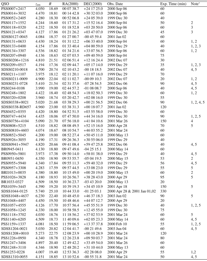
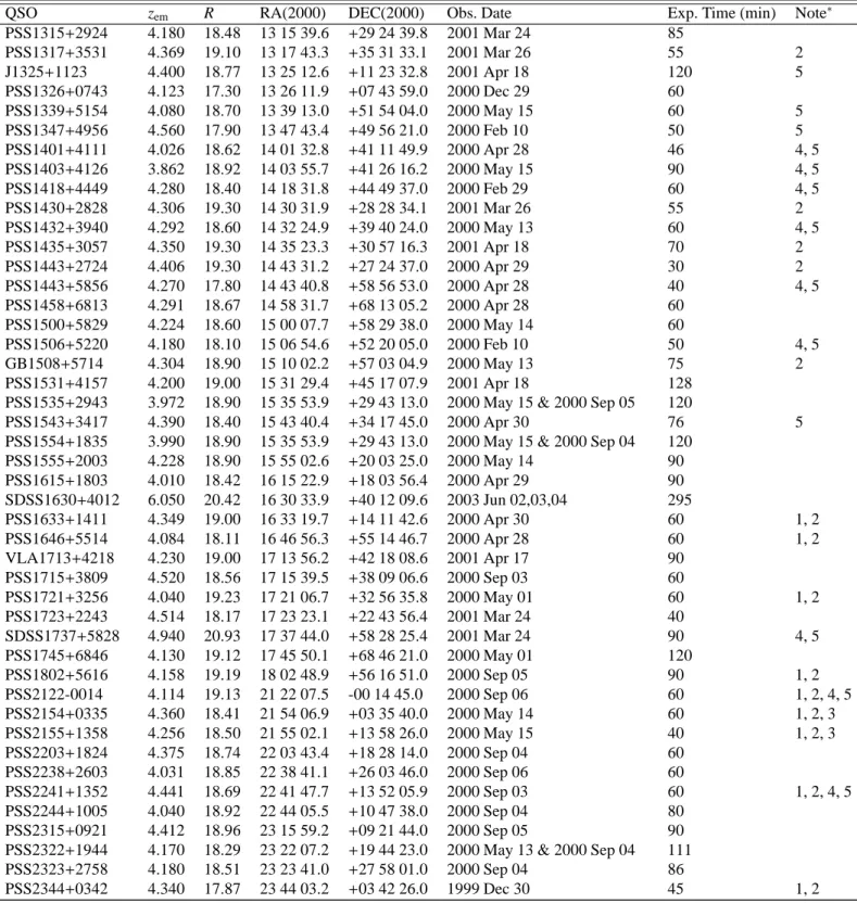
Observatory Sky Survey; see, e.g., Kennefick et al. 1995, Djorgovski et al. 1999 and the complete listing of QSOs avail-able at http://www.astro.caltech.edu/∼george/z4.qsos) have been obtained with the Echellette Spectrograph and Imager (ESI, Sheinis et al 2002) mounted on the KECK II 10 m tele-scope. In total, 99 quasars have been observed, 57 of which already reported in the literature (see Table 1 for details). We provide in Table 1 a summary of the observation log for the 99 quasars. Columns 1 to 8 give, respectively, the quasar’s name, the emission redshift, the apparent R magnitude, the J2000 quasar coordinates, the date of observation, the exposure time and the notes.
The echelle mode allows to cover the full wavelength range from 3900 Å to 10900 Å in ten orders with ∼ 300 Å overlap between two adjacent orders. The instrument has a spectral dis-persion of about 11.4 km s−1 pixel−1 and a pixel size ranging
from 0.16 Å pixel−1 in the blue to 0.38 Å pixel−1 in the red.
The 1 arcsec wide slit is projected onto 6.5 pixel resulting in a
R ∼4300 spectral resolution.
Data reduction followed standard procedures using IRAF for 70% of the sample and the programme makee for the re-maining. For the IRAF reduction, the procedure was as follows. The images were overscan corrected for the dual-amplifier mode. Each amplifier has a different baseline value and differ-ent gain which were corrected by using a script adapted from LRIS called esibias. Then all the images were bias subtracted and corrected for bad pixels. The images were divided by a nor-malized two-dimensional flat-field image to remove individual pixel sensitivity variations. The flat-field image was normal-ized by fitting its intensity along the dispersion direction using a high order polynomial fit, while setting all points outside the order aperture to unity. The echelle orders were traced using the spectrum of a bright star. Cosmic rays were removed from all two-dimensional images. For each exposure the quasar spec-trum was optimally extracted and background subtracted. The task apall in the IRAF package echelle was used to do this. The CuAr lamps were individually extracted using the quasar’s apertures. Lines were identified in the arc lamp spectra by us-ing the task ecidentify and a polynomial was fitted to the line positions resulting in a dispersion solution with a mean RMS of 0.09 Å. The dispersion solution computed on the lamp was then assigned to the object spectra by using the task dispcor. Wavelengths and redshifts were computed in the heliocentric restframe. The different orders of the spectra were combined using the task scombine in the IRAF package. It is important to note that the signal-to-noise ratio drops sharply at the edges of the orders. We have therefore carefully controlled this pro-cedure to avoid any spurious feature.
The SNR per pixel was obtained in the regions of the Lyman-α forest that are free of absorption and the mean SNR value, averaged between the Lyman-α and Lyman-β QSO emis-sion lines, was computed. We used only spectra with mean SNR ≥ 10. For simplicity, we excluded from our analysis broad absorption line (BAL) quasars. We therefore used 77 lines-of-sight out of the 99 available to us.
The continuum was automatically fitted (Aracil et al. 2004; Guimar˜aes et al. 2007) and the spectra were normalized. We checked the normalization for all lines-of-sight and
manu-ally corrected for local defects especimanu-ally in the vicinity of the Lyman-α emission lines and when the Lyman-α forest is strongly blended.
Metallicities measured for twelve z > 3 DLAs observed along five lines-of-sight of this sample have been published by Prochaska et al. (2003b); see also Prochaska et al. (2003a).
3. Identification of Damped and sub-Damped
Lyman-
α
systemsWe used an automatic version of the Voigt profile fitting routine VPFIT (Carswell et al. 1987) to decompose the Lyman-α forest of the spectra in individual components. As usual, we restricted our search outside of 3000 km s−1from the QSO emission
red-shift. This is to avoid contamination of the study by proximate effects such as the presence of overdensities around quasars (e.g. Rollinde et al. 2005, Guimar˜aes et al. 2007).
From this fit we could identify the candidates with log N(H i) − error ≥ 19.5. We then carefully inspected each of these candidates individually with special attention to the following characteristics of DLA absorption lines:
– the wavelength range over which the line is going to zero; – the presence of damped wings;
– the identification of associated metal lines when possible.
The redshift of the H i absorptions was adjusted carefully using the associated metal absorption features and the final H i col-umn density was then refitted using the high order lines in the Lyman series when Lyman series are covered by our spectrum and not blended with other lines. After applying the above cri-teria, 100 DLAs and sub-DLAs with log N(H i) ≥ 19.5 were confirmed. A total of 65 systems were not previously used for
ΩDLA,HI/Ωsub−DLA,HI estimations, 21 of which are DLAs and
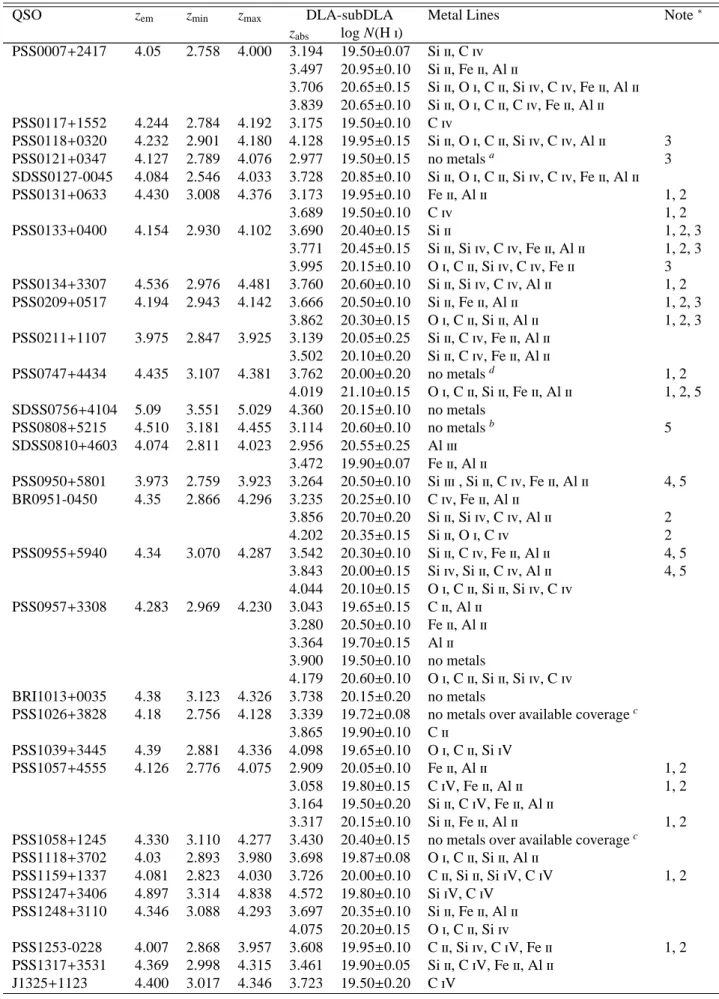
44 are sub-DLAs. Their characteristics are given in Table 2: Columns 1 to 7 give, respectively, the QSO’s name; the emis-sion redshift estimated as the average of the determinations from the peak of the Lyα emission and from the peak of a Gaussian fitted to the CIV emission line; the minimum red-shift along a DLA/sub-DLA could be detected; the maximum redshift along a DLA/sub-DLA could be detected; the redshift of the DLA/sub-DLA; the DLA/sub-DLA H i column den-sity; associated detected metal lines and notes. Lyman series and selected associated metal lines are shown in the Appendix ”List of Figures”. The QSO lines of sight of our sample along which we detect no DLA and/or sub-DLA are listed in Table 3. Comments on DLA/sub-DLA systems differences between our measurements and measurements by others are in the Appendix ”Notes on Individual Systems”.
The metal lines have been searched for using a search list of the strongest atomic transitions given in Table 4. The corresponding absorptions have been fitted using the package VPFIT. A full account of this metallic column densities and the corresponding abundances is out of the scope of this paper and will be presented elsewhere (Guimar˜aes et al., in preparation).
4. Analysis
Using the procedure described in the previous Section, we de-tect 100 systems with log N (H i) ≥ 19.5, out of which 40 are DLAs. We use this sample to investigate the characteristics of the neutral phase over the redshift range 2.5 ≤ z ≤ 5. We com-pare in Fig 1 the redshift sensitivity function of our survey with the redshift sensitivity function of previous surveys computed by PMSI03. Although the redshift path of our survey is much
0 50 100 150 200 250 300 350 0 1 2 3 4 5 g(z) z
Fig. 1. Solid curve shows the redshift sensitivity function of our survey for all lines-of-sight, the filled grey histogram is only for unpublished lines-of-sight. Dashed curve shows the redshift sensitivity function of previous surveys computed by PMSI03.
smaller than that of the SDSS survey (PHW05), it is at z > 3.5 similar to the surveys by P´eroux et al. (2001, 2003). Note that our survey is homogeneous and at spectral resolution twice or more larger than previous surveys. The H i column density dis-tribution of the 100 DLAs and sub-DLAs measured in this work and that of the systems with log N(H i) ≥ 20.3 in PMSI03 are shown in Fig. 2. We are confident that we do not miss a large number of sub-DLAs down to the above limit.
To give a global overview of the survey, we plot in Fig. 3, log N(H i) versus zabsfor the 65 unpublished damped/sub-DLA
absorption systems. In the same figure we show for comparison the data points from the P´eroux et al. (2001) survey.
In Figure 4, we plot for comparison, as a function of red-shift, the difference between the H i column densities measured for the same systems by us and by either P´eroux et al. (2005) from high-resolution data or Prochaska & Wolfe (2009) from SDSS data. The measurements are consistent within errors.
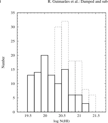
0 5 10 15 20 25 30 35 19.5 20 20.5 21 21.5 Number log N(HI)
Fig. 2. Histogram of the H i column densities measured for the 100 DLAs and sub-DLAs with log N(H i) ≥ 19.5 detected in our survey (solid-line histogram). The dashed-line histogram represents the H i column densities measured by PMSI03 with log N(H i) ≥ 20.3. 19 19.5 20 20.5 21 21.5 22 2.5 3 3.5 4 4.5 5 log N(HI) zabs This work Peroux et al. 2001
Fig. 3. The logarithm of the H i column density measured in our unpublished systems (circles) is plotted versus the redshift. The data points of P´eroux et al. (2001) are shown for comparison with crosses. -1 -0.8 -0.6 -0.4 -0.2 0 0.2 0.4 0.6 0.8 1 3 3.5 4 4.5 5 ∆ [N(HI)] zabs
Fig. 4. The H i column density difference between our mea-surements and those by either P´eroux et al. (2005) (triangles) or Prochaska & Wolfe (2009) (squares) in systems common to different surveys is plotted versus redshift.
4.1. Column Density Distribution Function
The H i absorption system frequency distribution function is defined as:
f (N, X)dNdX = msys
∆N ×Pni∆Xi
dNdX (1)
where msysis the number of absorption systems with a
col-umn density comprized between N − ∆N/2 and N + ∆N/2 and observed over an absorption distance interval of ∆X. The to-tal absorption distance coverage,Pni ∆Xi, is computed over the
whole sample of n QSO lines-of-sight. The absorption distance,
X, is defined as
X(z) =
Z z
0
(1 + z)2E(z)dz (2)
where E(z) = [ΩM(1 + z)3+ Ω∆]−1/2. For one line-of-sight, ∆X(z) = X(zmax)−X(zmin), with zmaxbeing the emission redshift
minus 3000 km s−1and z
minis the redshift of an H i Lyman-α
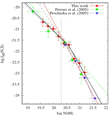
line located at the position of the QSO Lyman-β emission line. In Figure 5 we show the function f (N, X) obtained from our statistical sample over the redshift range z = 2.55 − 5.03 and for log N(H i) ≥ 19.5. It can be seen that there is no break at the low column density end, between log N(H i) = 19.5 and 20.6. This makes us confident that we are complete down to log N(H i) = 19.5. The vertical bars indicate 1σ errors. The horizontal bars indicate the bin sizes plotted at the mean col-umn density for each bin. PHW05 results in the redshift range
-24 -23.5 -23 -22.5 -22 -21.5 -21 -20.5 -20 19 19.5 20 20.5 21 21.5 22 log f HI (N,X) log N(HI) This work Peroux et al. (2005) Prochaska et al. (2005)
Fig. 5. Frequency distribution function over the redshift range
z = 2.55 − 5.03. The dashed green, solide black and dotted blue
lines are, respectively, a power-law, a double power-law and a gamma function fits to the data. The solid red and dashed black lines are, respectively, a power-law and gamma function fits to the data obtained by PHW05.
z = 2.2 − 5.5 and for logN(H i) ≥ 20.3 are overplotted in
the same figure. Although our data points are consistent within about 1σ with those of PHW05, it seems that the overwhole shape of the function is flatter in our data. Note that we do not detect any system with log N(H i) > 21.25. Data points from P´eroux et al. (2005), hereafter PDDKM05, are also overplot-ted. Our point at logN(H i) = 19.5 is consistent with theirs.
A law, a gamma function and/or a double power-law are usually used to fit the frequency distribution. It is ap-parent from Fig. 5 that a power-law (of the form f (N, X) =
K × N−α) fits the function nicely over the column density range 19.5 < log N(H i) < 21. The index of this power spectrum (see Table 5) is larger (α ∼ -1.4) than what is found by PHW05 but over a smaller column density range log N(H i) > 20.3. The discrepancy is apparently due to the difference in the col-umn density ranges considered by both studies. If we restrict our fit to the same range as PHW05 we find an index of α ∼ -1.8±0.25 which is consistent with the results of PHW05. We note that PDDKM05 already mentioned that the small end of the column density distribution is flatter than α = −2.
There is a large deficit of high column density systems in our survey compared to what would be expected from the sin-gle power-law fit. This has been noted before and discussed in detail by PHW05. A double power-law was used to fit our full sample with better result (see Table 5). However, the sharp break in the function at log N(H i) ∼ 21 suggests a gamma
func-tion of the form, f (N, X) = K × (NN
T)
−α×e−NTN (Pei & Fall 1995) should better describe the data.
We have calculated the frequency distribution function,
f (N, X), in different redshift bins of equal distance path :
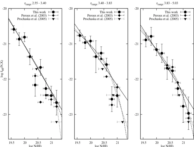
2.55−3.40; 3.40−3.83 and 3.83−5.03. Results are shown in Fig. 6. The functions are fitted as described above and fit results are given in Table 5. We find that the function do not evolve much with redshift. This is consistent with the finding by PHW05 that the global characteristics of the function are not changing much with time. There is however a tendancy for a flattening of the function which may indicate that the number of sub-DLAs relatively to other systems is larger at lower redshift. Although we do not think this is the case because we have used a con-servative approach, part of this evolution at the highest redshift could possibly be a consequence of loosing the sub-DLAs in the strongly blended Lyman-α forest at z > 4. We note also a slight decrease of the number of systems with log N(H i) > 20.5 at the highest redshifts. This is consistent with the finding by PDDKM05 that the relative number of high column density DLAs decreases with redshift.
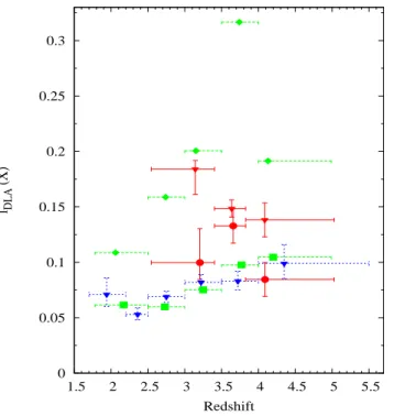
Another way to look at these variations is to compute the redshift evolution of the number of (sub)DLAs per unit path length. The observed density of systems is defined as
l(sub)DLAs=
Z Nmax
Nmin
f (N, X)dN (3)
Results obtained during the present survey together with those of PWH05 and PDDKM05 are plotted in Figure 7. The important feature of this plot is that the number density of DLAs peaks at z ∼ 3.5. In addition, the ratio of the number of sub-DLAs to the number of DLAs is larger at redshift <3.5 compared to higher redshifts.
4.2. Neutral hydrogen cosmological mass density,
Ω
HIThe comoving mass density of neutral gas is given by
ΩHI(z) = H0 c µmH ρ0 ΣiNi(HI) ∆X(z) (4)
where the density is in units of the current critical density
ρ0; mHis the mass of the hydrogen atom, µ = 1.3 is the mean
molecular weight, ∆X the absorption length and the summa-tion of column densities is done over all absorpsumma-tion systems detected in the survey. Results are shown in Fig. 8 and summa-rized in Table 6. The three redshift bins considered are defined so that the absorption length is equal in each bin. The different columns of Table 6 give, respectively, the redshift range, the mean redshift, the number of lines-of-sight involved, the num-ber of DLAs and sub-DLAs detected over this redshift range, the absorption length (calculated using zminand zmaxas defined
in Table 2), the resulting H i cosmological densities for, respec-tively, DLAs only or both DLAs and sub-DLAs.
Results from PHW05 and PDDKM05 are also plotted on Figure 8. It can be seen that we confirm the decrease of ΩHIfor
z > 3 that was noticed by PDDKM05. The measurement from
the SDSS in this redshift range is higher. However, our survey is of higher spectral resolution and should in principle be more
-23 -22 -21 -20 19.5 20 20.5 21 log f HI (N,X) log N(HI) zrange 2.55 - 3.40 This work Peroux et al. (2003) Prochaska et al. (2005) -23 -22 -21 -20 19.5 20 20.5 21 log N(HI) zrange 3.40 - 3.83 This work Peroux et al. (2003) Prochaska et al. (2005) -23 -22 -21 -20 19.5 20 20.5 21 log N(HI) zrange 3.83 - 5.03 This work Peroux et al. (2003) Prochaska et al. (2005)
Fig. 6. H i frequency distribution, fHI(N, X), in three redshifts bins: 2.55−3.40 (left), 3.40−3.83 (center), and 3.83−5.03 (right).
Straight lines show best χ2fits of a power-law function to the binned data. The dashed curve is the same for a gamma function
fit. and the dot-dashed curve for a double power-law fit.
reliable in this redshift range. It seems that the evolution of ΩHI
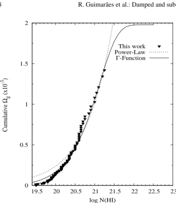
is a steep increase from z = 2 to z = 3 and then a slightly flatter decrease up to z = 5. The inclusion of the sub-DLAs does not change this picture as sub-DLAs contribute to a maximum of about 30% to the total H i mass. The contribution by sub-DLAs is better seen in Fig. 9 where we plot the cumulative density versus the maximum H i column density considered. As noted already by numerous authors, the discrepancy of measurements at z < 1.5 is still a problem.
It can be also seen from the Figure 8 that ΩHI are lower
than Ωstellar, the mass density in stars in local galaxies. We find
for the ratio of the peak value of ΩHI to Ωstellarfor this work R ∼0.45. Previous surveys, PDDKM05 and PHW05, have found for the ratio 0.37 and 0.40 respectively.
5. Discussion
We have presented the results of a survey for damped and sub-damped Lyman-α systems (logN(H i) ≥ 19.5) at z ≥ 2.55 along the lines-of-sight to 77 quasars with emission redshifts in the range 4 ≥ zem ≥6.3. In total 99 quasars were observed
but 22 lines-of-sight were not used because of not enough SNR and/or because of the presence of broad absorption lines.
Intermediate resolution (R ∼ 4300) spectra have been obtained with the Echellette Spectrograph and Imager (ESI) mounted on the Keck telescope. The damped Lyman-α absorptions are identified on the basis of (i) the width of the saturated absorp-tion, (ii) the presence of damped wings and (iii) the presence of metals at the corresponding redshift. The detection is run automatically but all lines are verified visually. A total of 100 systems with log N(H i) ≥ 19.5 are detected of which 40 sys-tems are Damped Lyman-α syssys-tems (log N(H i) ≥ 20.3) for an absorption length of ∆X = 378. Spectra are shown in Appendix. PHW05 have derived from SDSS data that the cosmolog-ical density of the neutral gas increases strongly by a factor close to two from z ∼ 2 to z ∼ 3.5. Beyond this redshift, measurements are more difficult because the Lyman-α forest is dense. Our measurements should be more reliable because of better spectral resolution. We show, consistently with the find-ings of PDDKM05, that the cosmological density of the neutral gas decreases at z > 3.5. The overall cosmological evolution seems therefore to have a peak at this redshift.
We find that the H i column density distribution does not evolve strongly from z ∼ 2.5 to z ∼ 4. The one power-law fit in the range log N(H i) > 20.3 gives an index of α = −1.80±0.25, consistent with previous determinations. However, we find that
0 0.05 0.1 0.15 0.2 0.25 0.3 1.5 2 2.5 3 3.5 4 4.5 5 5.5 lDLA (X) Redshift
Fig. 7. Number density of absorbers vs. redshift. Red circles and inverse triangles are from this work for DLAs and sub-DLAs, respectively. The values obtained by PWH05 (blue in-verse triangles) and PDDKM05 (green squares) for DLAs are overplotted. The green diamonds are the values obtained for log N(H i) > 19.0 by PDDKM05.
the fit over the column density range log N(H i) = 19.5−21 is quite flat (α ∼ 1.4). This probably indicates that the slope at the low-end is much flatter than −2. This power-law overpre-dicts data at the high-end and a second much steeper power-law (or a gamma function) is needed. The fraction of H i mass in sub-DLAs is of the order of 30%. Our data do not support the claim by PDDKM05 that the incidence of low column-density sytems is larger at high redshift. The number density of sub-DLAs seems to peak at z ∼ 3.5 as well.
It is apparent that statistical errors are still large in our sur-vey. It would be therefore of first importance to enlarge the sample of (sub)DLAs at high redshift. For this we need to go to fainter quasars however. The advent of X-shooter, a new gen-eration spectrograph at the VLT with a spectral resolution of
R = 6700 in the optical, should allow this to be done in a
rea-sonable amount of observing time.
Acknowledgements. SGD is supported by the NSF grant AST-0407448, and the Ajax Foundation. Cataloguing of DPOSS and dis-covery of PSS QSOs was supported by the Norris Foundation and other private donors. We thank E. Thi´ebaut, and D. Munro for freely distributing his yorick programming language (available at ftp://ftp-icf.llnl.gov:/pub/Yorick), which we used to implement our analysis. The authors wish to recognize and acknowledge the very significant cutural role and reverence that the summit of Mauna Kea has always had within the indigenous Hawaian community. We are most fortunate to have the opportunity to conduct observations from this mountain. We acknowledge the Keck support staff for their efforts in performing these observations. 0 1 2 3 4 5 6 0 1 2 3 4 5 Ωg (x 10 -3 ) Redshift
Fig. 8. Cosmological evolution of the H i mass density. For DLAs: red squares are the results of this work, green squares are from PDDKM05, blue inverse triangles from PHW05 and black triangles from Rao et al. (2005). For sub-DLAs: red cir-cles are this work (for systems with column densities ≥ 19.5), green circles obtained from PDDKM05 (for systems with col-umn densities ≥ 19.0) and blue circles obtained from PHW05 (as determined from the single power-law fit to the LLS fre-quency distribution function). The black circle are the mass density in stars in local galaxies (Fukugita et al. 1998).
References
Aracil, B., Petitjean, P., Pichon, C., & Bergeron, J. 2004, A&A, 419, 811
Carswell, R. F., Webb, J. K., Baldwin, J. A., & Atwood, B. 1987, ApJ, 319, 709
Dessauges-Zavadsky, M., P´eroux, C., Kim, T.-S., D’Odorico, S., & McMahon, R. G. 2003, MNRAS, 345, 447
Djorgovski, S. G., Odewahn, S. C., Gal, R. R., Brunner, R. J., & de Carvalho, R. R. 1999, in Weymann R. J., Storrie-Lombardi L. J., Sawicki M., Brunner R. J., eds, ASP Conf. Ser. Vol. 191, Photometric Redshifts and the Detection of High Redshift Galaxies. Astron. Soc. Pac., San Francisco, p. 179
Fukugita, M., Hogan, C. J. & Peebles, P. J. E. 1998, ApJ, 503, 518 Guimar˜aes, R., Petitjean, P., Rollinde, E., de Carvalho, R. R.,
Djorgovski, S. G., Srianand, R., Aghaee, A., & Castro, S. 2007, MNRAS, 377, 657
Kennefick, J. D., Djorgovski, S. G., & de Carvalho, R. R. 1995, AJ, 110, 2553
Meiring, J. D., Kulkarni, V. P., Lauroesch, J. T., P´eroux, C., Khare, P., York, D. G., & Crotts, A. P. S. 2008, MNRAS, 384, 1015 Pei, Y. C., & Fall, S. M. 1995, ApJ, 454, 69
P´eroux, C., Storrie-Lombardi, L. J., McMahon, R. G., Irwin, M., & Hook, I. M. 2001, AJ, 121, 1799
P´eroux, C., McMahon, R. G., Storrie-Lombardi, L. J., & Irwin, M. J. 2003, MNRAS, 346, 1103 (PMSI03)
0 0.5 1 1.5 2 19.5 20 20.5 21 21.5 22 22.5 23 Cumulative Ωg (x10 -3 ) log N(HI) This work Power-Law Γ-Function
Fig. 9. ΩHI is plotted as a function of the maximum log N(H i)
considered
P´eroux, C., Dessauges-Zavadsky, M., D’Odorico, S., Sun Kim, T., & McMahon, R. G. 2005, MNRAS, 363, 479 (PDDKM05) Petitjean, P., Webb, J. K., Rauch, M., Carswell, R. F., & Lanzetta, K.
1993, MNRAS, 262, 499
Prochaska, J. X., Castro, S., & Djorgovski, S. G. 2003, ApJS, 148, 317 Prochaska, J. X., Gawiser, E., Wolfe, A. M., Castro, S., & Djorgovski,
S. G. 2003, ApJ, 595, L9
Prochaska, J. X., Herbert-Fort, S., & Wolfe, A. M. 2005, ApJ, 635, 123 (PHW05)
Prochaska, J. X., & Wolfe, A. M. 2009, ApJ, 696, 1543
Rao, S. M., Turnshek, D. A., & Nestor, D. B. 2006, ApJ, 636, 610 Rollinde, E., Srianand, R., Theuns, T., Petitjean, P., & Chand, H. 2005,
MNRAS, 361, 1015
Sheinis, A. I., Bolte, M., Epps, H. W., Kibrick, R. I., Miller, J. S., Radovan, M. V., Bigelow, B. C., & Sutin, B. M. 2002, PASP, 114, 851
Storrie-Lombardi, L. J., & Wolfe, A. M. 2000, ApJ, 543, 552 Viegas, S. M. 1995, MNRAS, 276, 268
Wolfe, A. M., Turnshek, D. A., Smith, H. E., & Cohen, R. D. 1986, ApJS, 61, 249
Table 1. Summary of Observations
QSO zem R RA(2000) DEC(2000) Obs. Date Exp. Time (min) Note∗
PSS0007+2417 4.050 18.69 00 07 38.7 +24 17 25.0 2000 Sep 06 60 PSS0014+3032 4.470 18.81 00 14 42.8 +30 32 03.0 2000 Sep 06 60 PSS0052+2405 4.280 18.30 00 52 06.8 +24 05 39.0 1999 Dec 30 40 PSS0117+1552 4.244 18.60 01 17 31.2 +15 52 16.4 2000 Sep 04 50 2 PSS0118+0320 4.232 18.50 01 18 52.8 +03 20 50.0 2000 Sep 06 60 3 PSS0121+0347 4.127 17.86 01 21 26.2 +03 47 07.0 1999 Dec 30 45 3 SDSS0127-0045 4.084 18.37 01 27 00.7 -00 45 59.4 2001 Jan 02 60 PSS0131+0633 4.430 18.24 01 31 12.2 +06 33 40.0 2000 Sep 04 60 1, 2 PSS0133+0400 4.154 17.86 01 33 40.4 +04 00 59.0 1999 Dec 29 40 1, 2, 3 PSS0134+3307 4.536 18.82 01 34 21.6 +33 07 56.5 2000 Sep 06 60 1, 2 PSS0207+0940 4.136 18.63 02 07 03.5 +09 40 59.0 2000 Sep 04 75 SDSS0206+1216 4.810 21.51 02 06 51.4 +12 16 24.4 2002 Dec 07 30 PSS0209+0517 4.194 17.36 02 09 44.7 +05 17 14.0 1999 Dec 29 35 1, 2, 3 SDSS0210-0018 4.700 20.74 02 10 43.2 -00 18 18.5 2002 Dec 07 40 4, 5 PSS0211+1107 3.975 18.12 02 11 20.1 +11 07 16.0 1999 Dec 29 70 SDSS0211-0009 4.900 22.04 02 11 02.7 -00 09 10.3 2002 Dec 07 20 1, 2 SDSS0231-0728 5.410 21.54 02 31 37.6 -07 28 54.5 2002 Dec 06 90 4, 5 PSS0244-0108 3.990 19.00 02 44 57.2 -01 08 08.7 2000 Sep 06 40 4, 5 PSS0248+1802 4.422 18.40 02 48 54.3 +18 02 50.3 1999 Dec 30 60 1, 2 PSS0320+0208 3.960 18.74 03 20 42.7 +02 08 16.0 1999 Dec 30 55 SDSS0338+0021 5.020 21.68 03 38 29.3 +00 21 56.5 2002 Dec 06 90 1, 2, 4, 5 SDSS0338-RD657 4.960 23.00 03 38 31.3 +00 18 07.7 2001 Jan 02 120 PSS0452+0355 4.420 18.80 04 52 51.5 +03 55 58.0 1999 Dec 30 60 PSS0747+4434 4.435 18.06 07 47 50.0 +44 34 16.0 1999 Dec 30 90 1, 2, 5 SDSS0756+4104 5.090 21.70 07 56 18.0 +41 04 10.6 2001 Mar 26 150 4 PSS0808+5215 4.510 18.82 08 08 49.5 +52 15 16.0 2000 Apr 28 70 5 SDSS0810+4603 4.074 18.67 08 10 54.7 +46 03 55.2 2001 Mar 24 60 PSS0852+5045 4.200 19.00 08 52 27.4 +50 45 11.0 2000 May 13 60 PSS0926+3055 4.190 17.31 09 26 36.3 +30 55 06.0 1999 Dec 29 40 SDSS0941+5947 4.820 20.66 09 41 08.4 +59 47 25.8 2002 Dec 06 40 4, 5 BR0945-0411 4.130 18.80 09 47 49.6 -04 25 15.1 2000 May 14 60 PSS0950+5801 3.973 17.38 09 50 14.0 +58 01 38.0 1999 Dec 29 40 4, 5 BR0951-0450 4.350 18.90 09 53 55.7 -05 04 19.5 2000 May 15 53 2 PSS0955+5940 4.340 17.84 09 55 11.3 +59 40 32.0 1999 Dec 29 56 4, 5 PSS0957+3308 4.283 17.59 09 57 44.5 +33 08 23.0 1999 Dec 29 55 5 BRI1013+0035 4.380 18.80 10 15 49.0 +00 20 19.0 2000 May 15 60 2 PSS1026+3828 4.180 18.93 10 26 56.7 +38 28 43.0 2000 Apr 29 95 5 BR1033-0327 4.509 18.50 10 36 23.7 -03 43 20.0 2000 May 13 20 PSS1039+3445 4.390 19.20 10 39 19.3 +34 45 10.9 2001 Apr 18 150 5 SDSS1044-0125 5.740 25.10 10 44 33.0 -01 25 03.1 2000 Apr 28 & 2001 Jan 01,02 330
SDSS1048+4637 6.230 22.40 10 48 45.0 +46 37 18.3 2003 Jun 02 90 5 PSS1048+4407 4.450 19.50 10 48 46.6 +44 07 12.7 2000 Apr 29 20 PSS1057+4555 4.126 17.70 10 57 56.4 +45 55 51.9 1999 Dec 30 40 1, 2, 5 PSS1058+1245 4.330 18.00 10 58 58.5 +12 45 55.0 1999 Dec 30 75 PSS1118+3702 4.030 18.76 11 18 56.2 +37 02 53.9 2001 Mar 24 60 5 PSS1140+6205 4.509 18.73 11 40 09.6 +62 05 23.3 2000 May 14 60 4, 5 PSS1159+1337 4.081 18.50 11 59 06.5 +13 37 37.8 2000 Feb 10 55 1, 2, 5 SDSS1204-0021 5.030 20.82 12 04 41.7 -00 21 49.6 2003 Jun 04 60 4, 5 SDSS1208+0010 5.273 22.75 12 08 23.9 +00 10 28.9 2001 Mar 24 120 PSS1226+0950 4.340 18.78 12 26 23.8 +09 50 03.7 2001 Mar 24 80 PSS1247+3406 4.897 20.40 12 49 42.2 +33 49 54.0 2001 Mar 26 60 PSS1248+3110 4.346 18.90 12 48 20.2 +31 10 44.0 2000 May 13 60 PSS1253-0228 4.007 19.40 12 53 36.3 -02 28 08.0 2000 Apr 29 55 1,2 SDSS1310-0055 4.151 18.85 13 10 52.6 -00 55 31.8 2001 Mar 24 50 4, 5
Table 1. continued.
QSO zem R RA(2000) DEC(2000) Obs. Date Exp. Time (min) Note∗
PSS1315+2924 4.180 18.48 13 15 39.6 +29 24 39.8 2001 Mar 24 85 PSS1317+3531 4.369 19.10 13 17 43.3 +35 31 33.1 2001 Mar 26 55 2 J1325+1123 4.400 18.77 13 25 12.6 +11 23 32.8 2001 Apr 18 120 5 PSS1326+0743 4.123 17.30 13 26 11.9 +07 43 59.0 2000 Dec 29 60 PSS1339+5154 4.080 18.70 13 39 13.0 +51 54 04.0 2000 May 15 60 5 PSS1347+4956 4.560 17.90 13 47 43.4 +49 56 21.0 2000 Feb 10 50 5 PSS1401+4111 4.026 18.62 14 01 32.8 +41 11 49.9 2000 Apr 28 46 4, 5 PSS1403+4126 3.862 18.92 14 03 55.7 +41 26 16.2 2000 May 15 90 4, 5 PSS1418+4449 4.280 18.40 14 18 31.8 +44 49 37.0 2000 Feb 29 60 4, 5 PSS1430+2828 4.306 19.30 14 30 31.9 +28 28 34.1 2001 Mar 26 55 2 PSS1432+3940 4.292 18.60 14 32 24.9 +39 40 24.0 2000 May 13 60 4, 5 PSS1435+3057 4.350 19.30 14 35 23.3 +30 57 16.3 2001 Apr 18 70 2 PSS1443+2724 4.406 19.30 14 43 31.2 +27 24 37.0 2000 Apr 29 30 2 PSS1443+5856 4.270 17.80 14 43 40.8 +58 56 53.0 2000 Apr 28 40 4, 5 PSS1458+6813 4.291 18.67 14 58 31.7 +68 13 05.2 2000 Apr 28 60 PSS1500+5829 4.224 18.60 15 00 07.7 +58 29 38.0 2000 May 14 60 PSS1506+5220 4.180 18.10 15 06 54.6 +52 20 05.0 2000 Feb 10 50 4, 5 GB1508+5714 4.304 18.90 15 10 02.2 +57 03 04.9 2000 May 13 75 2 PSS1531+4157 4.200 19.00 15 31 29.4 +45 17 07.9 2001 Apr 18 128 PSS1535+2943 3.972 18.90 15 35 53.9 +29 43 13.0 2000 May 15 & 2000 Sep 05 120
PSS1543+3417 4.390 18.40 15 43 40.4 +34 17 45.0 2000 Apr 30 76 5 PSS1554+1835 3.990 18.90 15 35 53.9 +29 43 13.0 2000 May 15 & 2000 Sep 04 120
PSS1555+2003 4.228 18.90 15 55 02.6 +20 03 25.0 2000 May 14 90 PSS1615+1803 4.010 18.42 16 15 22.9 +18 03 56.4 2000 Apr 29 90 SDSS1630+4012 6.050 20.42 16 30 33.9 +40 12 09.6 2003 Jun 02,03,04 295 PSS1633+1411 4.349 19.00 16 33 19.7 +14 11 42.6 2000 Apr 30 60 1, 2 PSS1646+5514 4.084 18.11 16 46 56.3 +55 14 46.7 2000 Apr 28 60 1, 2 VLA1713+4218 4.230 19.00 17 13 56.2 +42 18 08.6 2001 Apr 17 90 PSS1715+3809 4.520 18.56 17 15 39.5 +38 09 06.6 2000 Sep 03 60 PSS1721+3256 4.040 19.23 17 21 06.7 +32 56 35.8 2000 May 01 60 1, 2 PSS1723+2243 4.514 18.17 17 23 23.1 +22 43 56.4 2001 Mar 24 40 SDSS1737+5828 4.940 20.93 17 37 44.0 +58 28 25.4 2001 Mar 24 90 4, 5 PSS1745+6846 4.130 19.12 17 45 50.1 +68 46 21.0 2000 May 01 120 PSS1802+5616 4.158 19.19 18 02 48.9 +56 16 51.0 2000 Sep 05 90 1, 2 PSS2122-0014 4.114 19.13 21 22 07.5 -00 14 45.0 2000 Sep 06 60 1, 2, 4, 5 PSS2154+0335 4.360 18.41 21 54 06.9 +03 35 40.0 2000 May 14 60 1, 2, 3 PSS2155+1358 4.256 18.50 21 55 02.1 +13 58 26.0 2000 May 15 40 1, 2, 3 PSS2203+1824 4.375 18.74 22 03 43.4 +18 28 14.0 2000 Sep 04 60 PSS2238+2603 4.031 18.85 22 38 41.1 +26 03 46.0 2000 Sep 06 60 PSS2241+1352 4.441 18.69 22 41 47.7 +13 52 05.9 2000 Sep 03 60 1, 2, 4, 5 PSS2244+1005 4.040 18.92 22 44 05.5 +10 47 38.0 2000 Sep 04 80 PSS2315+0921 4.412 18.96 23 15 59.2 +09 21 44.0 2000 Sep 05 90 PSS2322+1944 4.170 18.29 23 22 07.2 +19 44 23.0 2000 May 13 & 2000 Sep 04 111 PSS2323+2758 4.180 18.51 23 23 41.0 +27 58 01.0 2000 Sep 04 86
PSS2344+0342 4.340 17.87 23 44 03.2 +03 42 26.0 1999 Dec 30 45 1, 2 ∗Quasars from this survey were previously used for Ω
DLA,HIestimations by: (1) P´eroux et al. (2001);
Table 2. List of DLA-subDLAs
QSO zem zmin zmax DLA-subDLA Metal Lines Note∗
zabs log N(H i)
PSS0007+2417 4.05 2.758 4.000 3.194 19.50±0.07 Si ii, C iv 3.497 20.95±0.10 Si ii, Fe ii, Al ii
3.706 20.65±0.15 Si ii, O i, C ii, Si iv, C iv, Fe ii, Al ii 3.839 20.65±0.10 Si ii, O i, C ii, C iv, Fe ii, Al ii PSS0117+1552 4.244 2.784 4.192 3.175 19.50±0.10 C iv
PSS0118+0320 4.232 2.901 4.180 4.128 19.95±0.15 Si ii, O i, C ii, Si iv, C iv, Al ii 3 PSS0121+0347 4.127 2.789 4.076 2.977 19.50±0.15 no metalsa 3
SDSS0127-0045 4.084 2.546 4.033 3.728 20.85±0.10 Si ii, O i, C ii, Si iv, C iv, Fe ii, Al ii PSS0131+0633 4.430 3.008 4.376 3.173 19.95±0.10 Fe ii, Al ii 1, 2
3.689 19.50±0.10 C iv 1, 2
PSS0133+0400 4.154 2.930 4.102 3.690 20.40±0.15 Si ii 1, 2, 3 3.771 20.45±0.15 Si ii, Si iv, C iv, Fe ii, Al ii 1, 2, 3 3.995 20.15±0.10 O i, C ii, Si iv, C iv, Fe ii 3 PSS0134+3307 4.536 2.976 4.481 3.760 20.60±0.10 Si ii, Si iv, C iv, Al ii 1, 2 PSS0209+0517 4.194 2.943 4.142 3.666 20.50±0.10 Si ii, Fe ii, Al ii 1, 2, 3
3.862 20.30±0.15 O i, C ii, Si ii, Al ii 1, 2, 3 PSS0211+1107 3.975 2.847 3.925 3.139 20.05±0.25 Si ii, C iv, Fe ii, Al ii
3.502 20.10±0.20 Si ii, C iv, Fe ii, Al ii
PSS0747+4434 4.435 3.107 4.381 3.762 20.00±0.20 no metalsd 1, 2
4.019 21.10±0.15 O i, C ii, Si ii, Fe ii, Al ii 1, 2, 5 SDSS0756+4104 5.09 3.551 5.029 4.360 20.15±0.10 no metals
PSS0808+5215 4.510 3.181 4.455 3.114 20.60±0.10 no metalsb 5
SDSS0810+4603 4.074 2.811 4.023 2.956 20.55±0.25 Al iii 3.472 19.90±0.07 Fe ii, Al ii
PSS0950+5801 3.973 2.759 3.923 3.264 20.50±0.10 Si iii , Si ii, C iv, Fe ii, Al ii 4, 5 BR0951-0450 4.35 2.866 4.296 3.235 20.25±0.10 C iv, Fe ii, Al ii
3.856 20.70±0.20 Si ii, Si iv, C iv, Al ii 2 4.202 20.35±0.15 Si ii, O i, C iv 2 PSS0955+5940 4.34 3.070 4.287 3.542 20.30±0.10 Si ii, C iv, Fe ii, Al ii 4, 5
3.843 20.00±0.15 Si iv, Si ii, C iv, Al ii 4, 5 4.044 20.10±0.15 O i, C ii, Si ii, Si iv, C iv
PSS0957+3308 4.283 2.969 4.230 3.043 19.65±0.15 C ii, Al ii 3.280 20.50±0.10 Fe ii, Al ii 3.364 19.70±0.15 Al ii 3.900 19.50±0.10 no metals
4.179 20.60±0.10 O i, C ii, Si ii, Si iv, C iv BRI1013+0035 4.38 3.123 4.326 3.738 20.15±0.20 no metals
PSS1026+3828 4.18 2.756 4.128 3.339 19.72±0.08 no metals over available coveragec
3.865 19.90±0.10 C ii
PSS1039+3445 4.39 2.881 4.336 4.098 19.65±0.10 O i, C ii, Si iV
PSS1057+4555 4.126 2.776 4.075 2.909 20.05±0.10 Fe ii, Al ii 1, 2 3.058 19.80±0.15 C iV, Fe ii, Al ii 1, 2 3.164 19.50±0.20 Si ii, C iV, Fe ii, Al ii
3.317 20.15±0.10 Si ii, Fe ii, Al ii 1, 2 PSS1058+1245 4.330 3.110 4.277 3.430 20.40±0.15 no metals over available coveragec PSS1118+3702 4.03 2.893 3.980 3.698 19.87±0.08 O i, C ii, Si ii, Al ii
PSS1159+1337 4.081 2.823 4.030 3.726 20.00±0.10 C ii, Si ii, Si iV, C iV 1, 2 PSS1247+3406 4.897 3.314 4.838 4.572 19.80±0.10 Si iV, C iV
PSS1248+3110 4.346 3.088 4.293 3.697 20.35±0.10 Si ii, Fe ii, Al ii 4.075 20.20±0.15 O i, C ii, Si iv
PSS1253-0228 4.007 2.868 3.957 3.608 19.95±0.10 C ii, Si iv, C iV, Fe ii 1, 2 PSS1317+3531 4.369 2.998 4.315 3.461 19.90±0.05 Si ii, C iV, Fe ii, Al ii
Table 2. continued.
QSO zem zmin zmax DLA-subDLA Metal Lines Note∗
zabs log N(H i) 4.133 19.50±0.20 no metalsb PSS1326+0743 4.123 2.866 4.072 2.919 19.95±0.10 Al ii 3.425 19.90±0.15 Al ii PSS1432+3940 4.292 3.105 4.239 3.274 21.00±0.15 C iv, Fe ii, Al ii PSS1435+3057 4.35 2.942 4.297 3.267 20.05±0.10 C iv, Al ii 3.516 20.20±0.10 Si ii, C iv, Al ii 3.778 19.85±0.10 C iv, Al ii
PSS1443+2724 4.406 3.095 4.352 4.223 20.90±0.15 Si iv, Si ii, C iv, Fe ii, Al ii 2 PSS1500+5829 4.224 3.031 4.172 3.585 19.55±0.10 no metals over available coveragec
3.915 20.50±0.10 O i
PSS1506+5220 4.18 3.275 4.128 3.223 20.70±0.10 Si ii, C iv, Fe ii, Al ii, Al iii PSS1531+4157 4.20 2.868 4.148 3.657 19.55±0.15 Si ii, C iv, Al ii
PSS1535+2943 3.972 2.797 3.922 3.202 20.60±0.10 Si ii, C iv, Fe ii, Al ii 3.762 20.55±0.15 O i, C ii, Si iv, C iv, Al ii PSS1554+1835 3.99 2.769 3.940 2.919 20.00±0.15 Si ii, C iv, Al ii, Al iii
PSS1555+2003 4.228 2.824 4.176 3.427 19.90±0.10 no metals over available coveragec PSS1633+1411 4.349 2.836 4.296 2.880 20.30±0.15 Fe ii, Si ii
PSS1646+5514 4.084 2.800 4.033 2.932 19.50±0.10 no metals over available coveragec
4.029 19.80±0.15 no metals over available coveragec
PSS1715+3809 4.52 3.004 4.465 3.341 21.05±0.20 Si ii, Fe ii, Al ii PSS1723+2243 4.515 3.062 4.460 3.697 20.35±0.10 Si ii, C iv, Fe ii, Al ii SDSS1737+5828 4.94 3.383 4.881 4.152 19.85±0.15 Si ii, Al ii
4.741 20.65±0.15 Si ii, O i, C ii 4, 5 PSS1745+6846 4.13 2.860 4.079 3.706 19.73±0.09 Si ii, C iv, Al iii
PSS1802+5616 4.158 2.821 4.106 3.391 20.25±0.10 Si iv, Si ii, C iv, Fe ii, Al ii 1, 2 3.554 20.40±0.10 O i, Si ii, C iv, Fe ii, Al ii 1, 2 3.762 20.65±0.15 C ii, Si ii, Fe ii, Al ii 1, 2 3.811 20.35±0.15 C ii, Si iv, Si ii, Al ii 1, 2 PSS2122-0014 4.114 2.903 4.063 3.207 20.20±0.10 Si ii, C iv, Fe ii, Al ii 1, 2, 4, 5
3.264 19.90±0.15 C iv, Al ii 4.001 20.15±0.15 C ii, Si iv, C iv 1, 2 PSS2155+1358 4.256 3.064 4.203 3.143 19.90±0.20 Fe ii, Al ii 3.318 20.75±0.20 Si ii, Fe ii, Al ii 1, 2 4.211 20.00±0.10 Si ii, O i, C ii PSS2203+1824 4.375 2.850 4.321 3.610 19.70±0.15 Si ii, C iv, Al ii 4.107 19.80±0.15 C ii, Si ii, Fe ii, Al ii
PSS2238+2603 4.031 2.816 3.981 3.857 20.45±0.15 Si ii, O i, C ii, Si iv, C iv, Fe ii, Al ii PSS2241+1352 4.441 3.106 4.387 3.656 20.15±0.20 Al ii, Si ii 1, 2
4.281 20.75±0.15 Si ii, O i, C ii, Fe ii, Al ii 1, 2, 4, 5 PSS2315+0921 4.412 2.863 4.358 3.220 21.25±0.15 C ii, Si ii, Fe ii, Al ii
3.425 21.00±0.20 Si ii, C iv, Fe ii, Al ii PSS2322+1944 4.17 2.754 4.118 2.888 19.95±0.10 Fe ii, Al ii
2.975 19.80±0.10 Fe ii, Al ii PSS2323+2758 4.18 2.823 4.128 2.952 19.80±0.10 no metals 3.684 20.60±0.15 Si ii, Fe ii
PSS2344+0342 4.340 2.939 4.287 3.220 21.20±0.10 no metals over available coveragec,d 1, 2
3.884 19.80±0.10 no metals over available coveragec,e aMetals were detected by P´eroux et al. (2005)
bMetals were detected by Prochaska & Wolfe (2009) cWe do not cover the red part of the spectrum λ ≥ 6400 Å dMetals were detected by P´eroux et al. (2001)
eMetals were detected by Dessauges-Zavadsky et al. (2003)
∗
Table 3. QSOs without detected DLAs and/or sub-DLAs
QSO zem zmin zmax Note∗
PSS0014+3032 4.470 2.866 4.415 SDSS0210-0018 4.700 3.177 4.643 4, 5 PSS0248+1802 4.430 3.118 4.376 2 PSS0452+0355 4.395 3.115 4.341 PSS0852+5045 4.216 2.939 4.164 PSS0926+3055 4.198 2.951 4.146 SDSS0941+5947 4.820 3.322 4.762 4, 5 PSS1140+6205 4.509 3.113 4.454 4, 5 SDSS1310-0055 4.152 2.830 4.101 4, 5 PSS1339+5154 4.080 2.783 4.029 5 PSS1401+4111 4.026 2.866 3.976 4, 5 PSS1403+4126 3.862 2.866 3.813 4, 5 PSS1418+4449 4.323 2.974 4.270 4, 5 PSS1430+2828 4.306 2.811 4.253 2 PSS1458+6813 4.291 2.990 4.238 GB1508+5714 4.304 3.217 4.251 2 PSS1543+3417 4.407 3.071 4.353 5 PSS1615+1803 4.010 2.783 3.960 PSS1721+3256 4.040 2.802 3.990 1, 2 PSS2154+0335 4.359 3.400 4.305 1, 2, 3 PSS2244+1005 4.040 2.810 3.990 ∗
Quasars from this survey were previously used for ΩDLA,HI estimations by: (1) P´eroux et al. (2001); (2) P´eroux et al. (2003)
(3)P´eroux et al. (2005); (4) Prochaska et al. (2005); Prochaska & Wolfe (2009)
Table 4. Principal absorption metal lines most frequently detected associated to high column density absorption systems.
Ion λ0(Å) fa logλ0f + log[N/N(H)]⊙+ 12.00
Si iii 1206.500 0.221 10.87 H i 1215,6701 0.4162 14.70 N v 1238.821 0.152 10.24 N v 1242.804 0.0757 9.93 Si ii 1260.4223 0.959 10.65 O i 1302,1685 0.0486 10.67 Si ii 1304,3702 0.147 9.85 C ii 1334,5323 0.118 10.85 Si iv 1393.76018 0.528 10.44 Si iv 1402.770 0.262 10.13 Si ii 1526,70698 0.23 10.11 C iv 1548.2041 0.194 11.13 C iv 1550.7812 0.097 10.83 Fe ii 1608.45085 0.062 9.52 Al ii 1670,7886 1.88 9.99 Al iii 1854.7164 0.539 9.49 Al iii 1862.7895 0.268 9.19 Fe ii 2344.2139 0.108 9.92 Fe ii 2374.4162 0.0395 9.49 Fe ii 2382.7652 0.328 10.41
Table 5. Frequency distribution fitting parameters
Form zrange log K α logNT β
Power-Law [2.55 - 5.03] 6.59±2.12 −1.384±0.105 ——- ——-[2.55 - 3.40] 5.55±2.88 −1.330±0.144 ——- ——-[3.40 - 3.83] 4.03±2.01 −1.056±0.199 ——- ——-[3.83 - 5.03] 4.38±2.39 −1.279±0.118 ——- ——-Double Power-Law [2.55 - 5.03] -21.78±0.31 −1.162±0.118 20.60±0.24 -2.07±0.51 [2.55 - 3.40] -22.64±1.25 −1.327±0.307 21.19±1.44 -5.98±2.07 [3.40 - 3.83] -21.28±0.19 −0.793±0.233 20.45±0.14 -2.49±0.74 [3.83 - 5.03] -21.63±0.25 −0.920±0.199 20.51±0.17 -2.10±0.44 Gamma [2.55 - 5.03] -21.95±0.36 −1.010±0.172 20.93±0.18 ——-[2.55 - 3.40] -22.53±1.54 −1.185±0.329 21.28±0.89 ——-[3.40 - 3.83] -20.96±0.28 −0.485±0.324 20.45±0.16 ——-[3.83 - 5.03] -21.80±0.35 −0.853±0.198 20.82±0.18
——-Table 6. Absorption Distance Path - Data for Figure 8
zrange <z > NQSO NDLA NsubDLA ∆X ΩDLA(103) ΩDLA+subDLA(103)
2.55 - 3.40 3.168 77 12 23 125.922 1.43 ± 0.33 1.71 ± 0.33 3.40 - 3.83 3.618 78 17 19 125.922 1.41 ± 0.26 1.65 ± 0.26 3.83 - 5.03 4.048 77 11 18 125.922 0.97 ± 0.22 1.21 ± 0.22
Appendix : Notes on individual systems
In this Appendix we discuss systems where we note differences between our measurements and measurements by others. 1. PSS 0131+0633 (zem= 4.430). P´eroux et al. (2001) report two sub-DLA candidates at zabs= 3.17 and 3.61 with log N(H i) =
19.9 and 19.8 respectively. For the second system however, P´eroux et al. (2001) give in Table 5 a redshift of zabs= 3.61 for
the H i line and zabs= 3.609 for the metal lines but a redshift of zabs= 3.69 and log N(H i) = 19.5 in their Section 8 namely,
”Notes on Individual Objects”. We also detect the first sub-DLA at zabs= 3.173 with logN(H i) = 19.95 ± 0.10. Metal lines
at that redshift are detected in the red part of the spectrum. For the second DLA candidate, we confirm the presence of the
zabs = 3.689 absorption with log N(H i) = 19.50 ± 0.10 in agreement with the sub-DLA candidate reported in Section 8 of
Peroux et al. (2001). Metal lines at that redshift are also observed in the red part of the spectrum.
2. PSS0747+4434 (zem= 4.435). P´eroux et al. (2001) report two DLA candidates at zrmabs= 3.76 and 4.02 with log N(H i) =
20.3 and 20.6 respectively, which are confirmed by our observations. We measure log N(H i) = 20.00 ± 0.20 at zabs= 3.762
and log N(H i) = 21.10 ± 0.15 at zabs = 4.019. No metal lines at zabs = 3.76 are observed in both surveys. We remind the
reader that our data are of higher spectral resolution.
3. SDSS 0756+4104 (zem= 5.09). We detect a sub-DLA candidate at zabs= 4.360 with log N(H i) = 20.15 ± 0.10. Although
no Lyman series and metals are detected for this system, the spectrum has a high enough SNR to fit the H i line well and to ascertain that this aborber is highly likely to be Damped.
4. BR 0951−450 (zem= 4.35). PMSI03 report the detection of two DLA candidates at zabs= 3.8580 and 4.2028 with log N(H i)
= 20.6 and 20.4 respectively, which are confirmed by our observations. We measure log N(H i) = 20.70 ± 0.20 at zabs= 3.856
and log N(H i) = 20.35 ± 0.15 at zabs= 4.202. We discover an additional Damped candidate at zabs= 3.235 with log N(H i)
= 20.25 ± 0.10. We believe that this system is not included in the statistical sample of PMSI03, because it falls below the
threshold of log N(H i) = 20.30. Metal lines at that redshift are observed in the red part of the spectrum.
5. BRI 1013+0035 (zem= 4.38). PMSI03 report one DLA candidate at zabs = 3.103 with log N(H i) = 21.1. This system is
not included in our sample since its redshift is smaller than the minimum redshift beyond which a DLA/sub-DLA could be detected in our spectrum. One Damped candidate was discovered at zabs= 3.738 with log N(H i) = 20.15 ± 0.20. We believe
that this system is not included in the statistical sample of PMSI03 because it falls below the threshold of log N(H i) = 20.30. Although no lyman series and metals are detected for this system, the SNR in the spectrum is high enough to ascertain that this absorber is highly likely to be Damped.
6. PSS 1057+4555 (zem= 4.126). P´eroux et al. (2001) report three DLA candidates at zabs= 2.90, 3.05 and 3.32 with log N(H i)
= 20.1, 20.3 and 20.2 respectively, which are confirmed by our observations. We measure log N(H i) = 20.05 ± 0.10 at
zabs = 2.909 , log N(H i) = 19.80 ± 0.15 at zabs = 3.058 and log N(H i) = 20.15 ± 0.10 at zabs = 3.317. Metal lines at
all three redshifts are observed in the red part of the spectrum. We report a new sub-DLA at zabs= 3.164 with log N(H i) =
19.50 ± 0.20. Several metal lines are detected for this sytem.
7. PSS 1253−0228 (zem = 4.007). P´eroux et al. (2001) report two DLA candidates at zabs = 2.78 and 3.60 with log N(H i)
= 21.4 and 19.7, respectively. The system at zabs = 2.78 is not included in our sample because its redshift falls below the
minimum redshift beyond which DLA/sub-DLA could be detected in our spectrum. We measure log N(H i) = 19.95 ± 0.10 at zabs= 3.608. Several metal lines are detected for this sytem.
8. J 1325+1123 (zem = 4.400). We have discovered two sub-DLA candidates at zabs = 3.723 and 4.133 with log N(H i) =
19.50 ± 0.20 and 19.50 ± 0.20, respectively. C iv metal lines are detected at zabs= 3.723. This two sub-DLAs can be found
in the list of SDSS DR5 systems available on Jason Prochaska’s website.
9. PSS 1633+1411 (zrmem= 4.349). P´eroux et al. (2001) report one sub-DLA candidate at zabs= 3.90 with log N(H i) = 19.8.
Here, we measure log N(H i) = 19.0 ± 0.20 at zabs = 3.909. We report a new DLA at zabs = 2.880 with log N(H i) =
20.30 ± 0.15. Several metal lines are detected for this sytem.
10. PSS 1646+5514 (zem= 4.084). No DLA candidate is detected by P´eroux et al. (2001) along this line of sight. We report here
two sub-DLA candidates at zabs= 2.932 and 4.029 with log N(H i) = 19.50 ± 0.10 and 19.80 ± 0.15, respectively. No metals
are seen over the available wavelength coverage.
11. PSS 2122−0014 (zem= 4.084). P´eroux et al. (2001) report two candidates at zabs= 3.20 and 4.00 with log N(H i) = 20.3 and
20.1, respectively. Here, we measure log N(H i) = 20.20 ± 0.10 and 20.15 ± 0.15 at zabs= 3.207 and 4.001. Several metal
lines are detected for both systems. We report a new sub-DLA candidate at zabs= 3.264 with log N(H i) = 19.90 ± 0.15.
Several metal lines are detected also for this system.
12. PSS 2154+0335 (zem= 4.359). P´eroux et al. (2001) report two candidates at zabs= 3.61 and 3.79 with log N(H i) = 20.4 and
19.70, respectively. No candidate with log N(H i) > 19.50 is detected in our spectrum.
13. PSS 2155+1358 (zem= 4.256). P´eroux et al. (2001) report one DLA at zabs= 3.32 with log N(H i) = 21.10. Dessauges et al.
(2003) report three sub-DLAs at zabs= 3.142, 3.565 and 4.212 with log N(H i) = 19.94, 19.37 and 19.61. Here, we measure
log N(H i) = 19.90 ± 0.20, 20.75 ± 0.20 and 20.00 ± 0.10 at zrmabs= 3.143, 3.318 and 4.211, respectively. Several metal lines
are detected for these systems.
14. PSS2344+0342 (zem = 4.340). P´eroux et al. (2001) report two DLAs at zabs= 2.68 and 3.21 with log N(H i) = 21.10 and
DLA/sub-DLA could be detected in our spectrum. We measure log N(H i) = 21.20 ± 0.10 at zabs= 3.220. Dessauges et al.
0 0.5 1 1.5 5100 Flux λ (°A)
Pss0007+2417 zabs= 3.194 log N(HI)= 19.50
Ly |α 0.5 1 6400 6405 6410 Flux λ (°A) Si II | 0 0.5 1 1.5 5400 5500 5600 Flux
Pss0007+2417 zabs= 3.497 log N(HI)= 20.95
Ly α | 0 0.5 1 1.5 4600 Flux Ly β | 0 0.5 1 1.5 7505 7510 7515 7520 Flux λ (°A) Al II | 0 0.5 1 1.5 5700 5800 Flux
Pss0007+2417 zabs= 3.706 log N(HI)= 20.65
Ly α | 0 0.5 1 1.5 4800 Flux Ly β | 0 0.5 1 1.5 6125 6130 Flux λ (°A) O I | 0 0.5 1 1.5 5800 5900 6000 Flux
Pss0007+2417 zabs= 3.839 log N(HI)= 20.65
Ly α | 0 0.5 1 1.5 4900 5000 Flux Ly β | 0.5 1 7775 7780 7785 7790 Flux λ (°A) Fe II | 0 0.5 1 1.5 5100 Flux
Pss0117+1552 zabs= 3.175 log N(HI)= 19.50
Ly α | 0.5 1 6460 6470 6480 6490 Flux λ (°A) C IV | | | | | | | | 0 0.5 1 1.5 6200 6300 Flux
Pss0118+0320 zabs= 4.128 log N(HI)= 19.95
Ly α | 0 0.5 1 1.5 6455 6460 6465 6470 Flux λ (°A) Si II | 0 0.5 1 1.5 4800 4900 Flux λ (°A)
Pss0121+0347 zabs= 2.977 log N(HI)= 19.50
Ly α | 0 0.5 1 1.5 5700 5800 Flux
Sdss0127-0045 zabs=3.728 log N(HI)= 20.85
Ly α | Ly α | 0 0.5 1 1.5 4800 4900 Flux Ly β | 0 0.5 1 1.5 6300 6305 6310 6315 Flux λ (°A) C II | 0 0.5 1 1.5 5000 5100 Flux
Pss0131+0633 zabs= 3.173 log N(HI)= 19.95
Ly α | 0.5 1 6965 6970 6975 6980 Flux λ (°A) Al II | 0 0.5 1 1.5 5700 Flux
Pss0131+0633 zabs= 3.689 log N(HI)= 19.50
Ly α | 0 0.5 1 1.5 7250 7260 7270 Flux λ (°A) C IV | | | | | | | | 0 0.5 1 1.5 5700 5800 5900 Flux λ (°A)
Pss0133+0400 zabs= 3.690-3.771 log N(HI)= 20.40-20.35
Ly α Ly α | | 0 0.5 1 1.5 5700 5800 5900 Flux λ (°A)
Pss0133+0400 zabs= 3.690-3.771 log N(HI)= 20.40-20.35
Fig. .1. Spectra of the 100 confirmed Lyman-α absorption with log N(H i) ≥ 19.5. In each panel the Voigt profile fit corresponding to the best N(H i) value is overplotted. The Lyman series absorption lines and one characteristic associated metal absorption feature (when metals are present over the available wavelength coverage and not blended with another lines) are presented in additional sub-panels.
0 0.5 1 1.5 4800 4900 Flux
Pss0133+0400 zabs= 3.690-3.771 log N(HI)= 20.40-20.35
Ly β Ly β | | 0 0.5 1 1.5 7160 Flux λ (°A) Si II | 7280 7290 λ (°A) Si II | 0 0.5 1 1.5 6000 6100 Flux
Pss0133+0400 zabs= 3.995 log N(HI)= 20.15
Ly α | 0 0.5 1 1.5 5100 Flux Ly β | 0.5 1 1.5 7725 7730 7735 7740 7745 7750 7755 Flux λ (°A) C IV | | | | 0 0.5 1 1.5 5700 5800 5900 Flux
Pss0134+3307 zabs= 3.760 log N(HI)= 20.60
Ly α | 0 0.5 1 1.5 4900 Flux Ly β | 0.5 1 1.5 7945 7950 7955 7960 Flux λ (°A) Al II | 0 0.5 1 1.5 5700 5800 5900 Flux
Pss0134+3307 zabs= 3.760 log N(HI)= 20.60
Ly α | 0 0.5 1 1.5 4900 Flux Ly β | 0.5 1 1.5 7945 7950 7955 7960 Flux λ (°A) Al II | 0 0.5 1 1.5 5600 5700 Flux
Pss0209+0517 zabs= 3.664 log N(HI)= 20.50
Ly α | 0.5 1 1.5 7115 7120 7125 Flux λ (°A) Si II | 0 0.5 1 1.5 5900 6000 Flux
Pss0209+0517 zabs= 3.862 log N(HI)= 20.30
Ly α | 0.5 1 1.5 7415 7420 7425 7430 Flux λ (°A) Si II | 0 0.5 1 1.5 5000 5100 Flux
Pss0211+1107 zabs= 3.139 log N(HI)= 20.05
Ly α | 0 0.5 1 1.5 6910 6915 6920 6925 Flux λ (°A)
Pss0211+1107 zabs= 3.139 log N(HI)= 20.05 AlII | 0 0.5 1 1.5 5400 5500 Flux
Pss0211+1107 zabs= 3.502 log N(HI)= 20.10
Ly α | 0 0.5 1 1.5 6965 6970 6975 6980 6985 6990 Flux λ (°A)
Pss0211+1107 zabs= 3.502 log N(HI)= 20.10
C IV | | | | 0 0.5 1 1.5 5700 5800 Flux λ (°A)
Pss0747+4434 zabs= 3.762 log N(HI)= 20.00
Ly α | 0 0.5 1 1.5 6000 6100 6200 Flux
Pss0747+4434 zabs= 4.019 log N(HI)= 21.10
Ly α | Ly α | 0 0.5 1 1.5 5100 5200 Flux Ly β | 0.5 1 1.5 8070 8075 8080 Flux λ (°A) Fe II | 0 0.5 1 1.5 6500 6600 Flux λ (°A)
Pss0756+4104 zabs= 4.360 log N(HI)= 20.15
Ly α | 0 0.5 1 1.5 6500 6600 Flux λ (°A)
Pss0756+4104 zabs= 4.360 log N(HI)= 20.15
Ly α |
0 0.5 1 1.5 4900 5000 5100 Flux λ (°A)
Pss0808+5215 zabs= 3.114 log N(HI)= 20.60
Ly α | 0 0.5 1 1.5 4700 4800 4900 Flux
Sdss0810+4603 zabs= 2.956 log N(HI)= 20.55
Ly α | 0.5 1 1.5 7340 7350 7360 7370 7380 Flux λ (°A) Al III | | 0 0.5 1 1.5 5400 5500 Flux
Sdss0810+4603 zabs= 3.472 log N(HI)= 19.90
Ly α | 0 0.5 1 1.5 6820 6825 6830 6835 Flux λ (°A) Fe II | 0 0.5 1 1.5 5100 5200 Flux
Pss0950+5801 zabs= 3.264 log N(HI)= 20.50
Ly α | 0 0.5 1 1.5 6500 6505 6510 6515 Flux λ (°A) Si II | 0 0.5 1 1.5 5100 5200 Flux λ (°A)
Br0951-0450 zabs= 3.235 log N(HI)= 20.25
0.5 1 1.5 7070 7075 7080 Flux λ (°A) Al II | 0 0.5 1 1.5 5800 5900 6000 Flux
Br0951-0450 zabs= 3.856 log N(HI)= 20.70
0 0.5 1 1.5 7510 7515 7520 7525 7530 7535 7540 Flux λ (°A) C IV | | 0 0.5 1 1.5 6300 6400 Flux
Br0951-0450 zabs=4.202 log N(HI)= 20.35
Ly α | 0 0.5 1 1.5 5300 5400 Flux Ly β | 0 0.5 1 1.5 5000 5100 Flux Ly γ | 0 0.5 1 1.5 6765 6770 6775 6780 Flux λ (°A) OI | | 0 0.5 1 1.5 5500 5600 Flux
Pss0955+5940 zabs= 3.542 log N(HI)= 20.30
Ly α | 0.5 1 1.5 7300 7305 7310 7315 Flux λ (°A) FeII | 0 0.5 1 1.5 5800 5900 Flux
Pss0955+5940 zabs=3.843 log N(HI)= 20.00
Ly α | 0 0.5 1 1.5 4900 5000 Flux Ly β | 0.5 1 1.5 7385 7390 7395 7400 Flux λ (°A) SiII | 0 0.5 1 1.5 6100 6200 Flux
Pss0955+5940 zabs= 4.044 log N(HI)= 20.10
Ly α | 0.5 1 1.5 7695 7700 7705 Flux λ (°A) SiII | 0 0.5 1 1.5 4900 Flux
Pss0957+3308 zabs= 3.043 log N(HI)= 19.65
Ly α | 0.5 1 1.5 6750 6755 Flux λ (°A) Al II | | 0.5 1 1.5 6750 6755 Flux λ (°A) Fig. .1. Continued.
0 0.5 1 1.5 5200 5300 Flux
Pss0957+3308 zabs= 3.280 log N(HI)= 20.50
Ly α | 0 0.5 1 1.5 7140 7145 7150 7155 Flux λ (°A) Al II | 0 0.5 1 1.5 5300 Flux
Pss0957+3308 zabs= 3.364 log N(HI)= 19.70
Ly α | 0.5 1 1.5 7285 7290 7295 Flux λ (°A) Al II | 0 0.5 1 1.5 5900 6000 Flux λ (°A)
Pss0957+3308 zabs= 3.900 log N(HI)= 19.50
Ly α | 0 0.5 1 1.5 6200 6300 6400 Flux
Pss0957+3308 zabs= 4.179 log N(HI)= 20.60
Ly α | 0 0.5 1 1.5 8010 8020 8030 Flux λ (°A) C IV | | 0 0.5 1 1.5 5700 5800 Flux λ (°A)
Bri1013+0035 zabs= 3.738 log N(HI)= 20.15
Ly α | 0 0.5 1 1.5 5300 Flux λ (°A)
Pss1026+3828 zabs= 3.339 log N(HI)= 19.72
Ly α | 0 0.5 1 1.5 5900 Flux
Pss1026+3828 zabs= 3.865 log N(HI)= 19.90
Ly α | 0.5 1 1.5 6485 6490 6495 6500 Flux λ (°A) C II | 0 0.5 1 1.5 6200 Flux
Pss1039+3445 zabs= 4.098 log N(HI)= 19.65
Ly α | 0 0.5 1 1.5 7100 7110 7120 7130 7140 7150 7160 Flux λ (°A) Si IV | | 0 0.5 1 1.5 4700 4800 Flux
Pss1057+4555 zabs= 2.909 log N(HI)= 20.05
Ly α | 0.5 1 1.5 6280 6285 6290 6295 Flux λ (°A) Fe II | 0 0.5 1 1.5 4900 5000 Flux λ (°A)
Pss1057+4555 zabs= 3.058 log N(HI)= 19.80
Ly α | 0.5 1 1.5 6280 6290 6300 6310 Flux λ (°A) C IV | | 0 0.5 1 1.5 5000 5100 Flux
Pss1057+4555 zabs= 3.164 log N(HI)= 19.50
Ly α | 0.5 1 1.5 6350 6355 6360 Flux λ (°A) Si II | 0 0.5 1 1.5 5200 5300 Flux
Pss1057+4555 zabs= 3.317 log N(HI)= 20.15
Ly α | 0 0.5 1 1.5 6580 6585 6590 6595 6600 Flux λ (°A) Si II | 0 0.5 1 1.5 5300 5400 Flux λ (°A)
Pss1058+1245 zabs= 3.430 log N(HI)= 20.40
Ly α | 0 0.5 1 1.5 5700 Flux
Pss1118+3702 zabs= 3.698 log N(HI)= 19.87
Ly α | 0.5 1 1.5 7165 7170 7175 7180 Flux λ (°A) Si II | 0.5 1 1.5 7165 7170 7175 7180 Flux λ (°A) Fig. .1. Continued
0 0.5 1 1.5 5700 5800 Flux
Pss1159+1337 zabs= 3.726 log N(HI)= 20.00
Ly α | 0 0.5 1 1.5 6295 6300 6305 6310 Flux λ (°A) C II | 0 0.5 1 1.5 6700 6800 Flux
Pss1247+3406 zabs= 4.572 log N(HI)= 19.80
Ly α | 0.5 1 1.5 7760 7770 7780 7790 7800 7810 Flux λ (°A) Si IV | | 0 0.5 1 1.5 5700 5800 Flux
Pss1248+3110 zabs= 3.697 log N(HI)= 20.35
Ly α | 0.5 1 1.5 7545 7550 7555 7560 7565 Flux λ (°A) Fe II | 0 0.5 1 1.5 6100 6200 Flux
Pss1248+3110 zabs= 4.075 log N(HI)= 20.20
Ly α | 0 0.5 1 1.5 5200 Flux λ (°A) Ly β | 0.5 1 1.5 7070 7080 7090 7100 7110 7120 Flux λ (°A)
Pss1248+3110 zabs= 4.075 log N(HI)= 20.20
Si IV | | 0 0.5 1 1.5 5600 Flux
Pss1253-0228 zabs= 3.608 log N(HI)= 19.95
Ly α | 0 0.5 1 1.5 6410 6420 6430 6440 6450 6460 Flux λ (°A) Si IV | | 0 0.5 1 1.5 5400 5500 Flux
Pss1317+3531 zabs= 3.461 log N(HI)= 19.90
Ly α | 0.5 1 6805 6810 6815 6820 Flux λ (°A) Si II | 0 0.5 1 1.5 5700 5800 Flux
J1325+1123 zabs= 3.723 log N(HI)= 19.50
Ly α | 0 0.5 1 1.5 7300 7310 7320 7330 Flux λ (°A) C IV | | 0 0.5 1 1.5 6200 6300 Flux
J1325+1123 zabs= 4.133 log N(HI)= 19.50
Ly α | 0 0.5 1 1.5 4700 4800 Flux
Pss1326+0743 zabs= 2.919 log N(HI)= 19.95
Ly α | 0 0.5 1 1.5 6540 6550 Flux λ (°A) Al II | | | 0 0.5 1 1.5 5300 5400 Flux
Pss1326+0743 zabs= 3.425 log N(HI)= 19.90
Ly α | 0.5 1 1.5 7390 7400 Flux λ (°A) Al II | 0 0.5 1 1.5 5100 5200 5300 Flux
Pss1432+3940 zabs= 3.274 log N(HI)= 21.00
Ly α | 0 0.5 1 1.5 7140 7150 Flux λ (°A) Al II | | | | 0 0.5 1 1.5 5100 5200 Flux
Pss1435+3057 zabs= 3.267 log N(HI)= 20.05
Ly α | 0.5 1 1.5 7130 7140 Flux λ (°A) Al II | 0.5 1 1.5 7130 7140 Flux λ (°A) Fig. .1. Continued
0 0.5 1 1.5 5400 5500 Flux
Pss1435+3057 zabs= 3.516 log N(HI)= 20.20
Ly α | 0.5 1 7540 7550 Flux λ (°A) Al II | 0 0.5 1 1.5 5800 Flux
Pss1435+3057 zabs= 3.778 log N(HI)= 19.85
Ly α | 0 0.5 1 1.5 7980 7990 Flux λ (°A) Al II | 0 0.5 1 1.5 6200 6300 6400 6500 Flux
Pss1443+3057 zabs= 4.223 log N(HI)= 20.90
Ly α | 0 0.5 1 1.5 5300 5400 Flux Ly β | 0 0.5 1 1.5 8400 8410 Flux λ (°A) Fe II | | 0 0.5 1 1.5 5600 Flux
Pss1500+5829 zabs= 3.585 log N(HI)= 19.55
Ly α | 0 0.5 1 1.5 5900 6000 Flux
Pss1500+5829 zabs= 3.915 log N(HI)= 20.50
Ly α | Ly α | 0 0.5 1 1.5 5000 5100 Flux Ly β | 0 0.5 1 1.5 6395 6400 6405 Flux λ (°A) O I | 0 0.5 1 1.5 5100 5200 Flux
Pss1506+5220 zabs= 3.223 log N(HI)= 20.70
Ly α | 0.5 1 1.5 7040 7045 7050 7055 7060 7065 Flux λ (°A) Al II | | | | 0 0.5 1 1.5 5600 5700 Flux
Pss1531+4157 zabs= 3.657 log N(HI)= 19.55
Ly α | 0.5 1 7105 7110 7115 7120 Flux λ (°A) Si II | 0 0.5 1 1.5 5000 5100 5200 Flux λ (°A)
Pss1535+2943 zabs= 3.202 log N(HI)= 20.60
0 0.5 1 1.5 6410 6415 6420 6425 Flux λ (°A)
Pss1535+2943 zabs= 3.202 log N(HI)= 20.60
Si II | 0 0.5 1 1.5 5700 5800 5900 Flux
Pss1535+2943 zabs= 3.762 log N(HI)= 20.50
Ly α | 0 0.5 1 1.5 4900 Flux Ly β | 0 0.5 1 1.5 6345 6350 6355 6360 Flux λ (°A) C II | 0 0.5 1 1.5 4700 4800 Flux
Pss1554+1835 zabs= 2.919 log N(HI)= 20.00
Ly α | 0 0.5 1 1.5 6540 6545 6550 6555 Flux λ (°A) Al II | 0 0.5 1 1.5 5400 Flux λ (°A)
Pss1555+2003 zabs= 3.427 log N(HI)= 19.90
Ly α | 0 0.5 1 1.5 4700 4800 Flux λ (°A)
Pss1633+1411 zabs= 2.880 log N(HI)= 20.30
Ly α | 0 0.5 1 1.5 4700 4800 Flux λ (°A)
Pss1633+1411 zabs= 2.880 log N(HI)= 20.30
Ly α |
0.5 1
7010 7015 7020 7025
Flux
λ (°A)
Pss1633+1411 zabs= 2.880 log N(HI)= 20.30
Si II | 0 0.5 1 1.5 4800 Flux λ (°A)
Pss1646+5514 zabs= 2.932 log N(HI)= 19.50
Ly α | 0 0.5 1 1.5 6100 Flux
Pss1646+5514 zabs=4.029 log N(HI)= 19.80
Ly α | 0 0.5 1 1.5 5100 5200 Flux
Pss1646+5514 zabs=4.029 log N(HI)= 19.80
Ly β | 0 0.5 1 1.5 4900 Flux λ (°A) Ly γ | 0 0.5 1 1.5 5200 5300 5400 Flux
Pss1715+3809 zabs= 3.341 log N(HI)= 21.05
Ly α | 0.5 1 6975 6980 6985 6990 Flux λ (°A) Fe II | 0 0.5 1 1.5 5700 5800 Flux λ (°A)
Pss1723+2243 zabs= 3.697 log N(HI)= 20.35
Ly α | 0 0.5 1 1.5 7835 7840 7845 7850 7855 7860 Flux λ (°A)
Pss1723+2243 zabs= 3.697 log N(HI)= 20.35
Al II || | | | | 0 0.5 1 1.5 6200 6300 Flux
Sdss1737+5828 zabs= 4.152 log N(HI)= 19.85
Ly α | 0.5 1 1.5 7860 7865 7870 Flux λ (°A) Si II | 0 0.5 1 1.5 6900 7000 Flux
Sdss1737+5828 zabs= 4.741 log N(HI)= 20.65
Ly α | 0 0.5 1 1.5 5900 Flux Ly β | 0.5 1 1.5 7470 7475 7480 7485 Flux λ (°A) O I | 0 0.5 1 1.5 5700 Flux
Ps1745+6846 zabs= 3.706 log N(HI)= 19.73
Ly α | 0.5 1 1.5 7180 7185 7190 7195 Flux λ (°A) Si II | 0 0.5 1 1.5 5300 5400 Flux
Pss1802+5616 zabs= 3.391 log N(HI)= 20.25
Ly α | 0.5 1 6795 6800 6805 6810 Flux λ (°A) C IV | | 0 0.5 1 1.5 5500 5600 Flux
Pss1802+5616 zabs= 3.554 log N(HI)= 20.40
Ly α | 0 0.5 1 1.5 7045 7050 7055 7060 7065 7070 Flux λ (°A) C IV | | 0 0.5 1 1.5 5700 5800 5900 Flux
Pss1802+5616 zabs= 3.762-3.811 log N(HI)= 20.65-20.35
Ly α Ly α | | 0 0.5 1 1.5 4800 4900 5000 Flux Ly β Ly β | | 0 0.5 1 1.5 7950 7960 Flux λ (°A) Al II | 7330 7340 λ (°A) Si II | 0 0.5 1 1.5 5100 5200 Flux λ (°A)
Pss2122-0014 zabs= 3.207 log N(HI)= 20.20
Ly α | 0 0.5 1 1.5 5100 5200 Flux λ (°A)
Pss2122-0014 zabs= 3.207 log N(HI)= 20.20
Ly α |