HAL Id: hal-00016855
https://hal.archives-ouvertes.fr/hal-00016855
Submitted on 12 Jan 2006HAL is a multi-disciplinary open access
archive for the deposit and dissemination of sci-entific research documents, whether they are pub-lished or not. The documents may come from
L’archive ouverte pluridisciplinaire HAL, est destinée au dépôt et à la diffusion de documents scientifiques de niveau recherche, publiés ou non, émanant des établissements d’enseignement et de
Bipartite Structure of All Complex Networks
Jean-Loup Guillaume, Matthieu Latapy
To cite this version:
Jean-Loup Guillaume, Matthieu Latapy. Bipartite Structure of All Complex Networks. Information Processing Letters, Elsevier, 2004, 90, pp.Issue 5, Pages 215-221. �10.1016/j.ipl.2004.03.007�. �hal-00016855�
Bipartite Structure
of all Complex Networks
Jean-Loup Guillaume and Matthieu Latapy
liafa
– cnrs – Universit´e Paris 7
2 place Jussieu, 75005 Paris, France.
(guillaume,latapy)@liafa.jussieu.fr
Abstract
The analysis and modelling of various complex networks has received much at-tention in the last few years. Some such networks display a natural bipartite struc-ture: two kinds of nodes coexist with links only between nodes of different kinds. This bipartite structure has not been deeply studied until now, mainly because it appeared to be specific to only a few complex networks. However, we show here that all complex networks can be viewed as bipartite structures sharing some important statistics, like degree distributions. The basic properties of complex networks can be viewed as consequences of this underlying bipartite structure. This leads us to propose the first simple and intuitive model for complex networks which captures the main properties met in practice.
Keywords: graphs, interconnection networks, modelling, bipartite graphs.
Context.
In a random network [7, 13] with n nodes, each of the n·(n−1)2 possible links exists with
a given probability p. In other words, a random network is constructed from n nodes by
choosing m = p · n·(n−1)2 links at random. Until recently, this model was the only one
available for the study of complex networks.
However, it has been shown recently [2, 11, 25, 29, 31] that this model does not capture some of the main features of complex networks observed in practice. In particular the clustering (probability that two nodes are connected, given that they are both connected to a same third) and the degree distribution (probability that a randomly chosen node has
k links, for each k) are inaccurate. Real-world complex networkshave a high clustering
and a heavy-tailed degree distribution (degrees variety can be spread over several orders of magnitudes), while random networks of comparable size have a clustering equal to p (which is small when the average degree is small) and a Poisson-shaped degree distribution (all nodes nearly have a typical degree). In many contexts, these properties have a strong influence on phenomena of interest [4, 21, 24, 27]. For surveys on the variety of complex networks and associated phenomena that have been studied, see [2, 8, 11, 25, 28, 29].
Various models have recently been proposed to capture the main properties met in practice. The first one [31] provides highly clusterized networks but the obtained degree distributions is still Poisson-shaped. Another important step was the introduction of the
preferential attachment principle [1, 12]: nodes are added one by one and link to
preex-isting nodes with a probability depending on the degree of these nodes. As explained in [1, 2, 6], this reflects the way a large variety of real-world networks are indeed constructed. The networks obtained have a power law degree distribution, but their clustering is much lower than in real-world networks.
Many other attempts have been made to produce networks having all the properties we have cited [2, 12, 26, 31]. However, none of them give at the same time an intuitive, realistic and simple interpretation of the causes of the observed properties. They either rely on artificial construction processes, produce networks which do not have all the desired properties, or are very difficult to analyze.
In this communication, we show that all complex networks have an underlying bipartite structure. This makes it possible to view their main properties as consequences of this underlying structure. This also leads to two very efficient models for the generation of complex networks having realistic properties. Moreover, these models can be studied both experimentally and analytically, and they give an interpretation of how these properties are induced by real-world construction processes. As we will discuss, all these aspects make these models interesting alternatives to those previously proposed.
Throughout our presentation, we will use a representative set of complex networks which have received much attention and span quite well the variety of context in which complex networks appear. The set consists of a protein network [9, 18], a map of the core of the Internet at router level [15, 16], the map of a large Web site (considered as undirected) [3, 9], the actors’ co-starring relation [10, 31], the co-occurrence relation of words [14] in the sentences of [30], and a co-authoring relation between scientists [5, 22, 23, 26]. We will refer to these networks as Proteins, Internet, Web, Actors, Cooccurrence, and Coauthoring respectively. They are precisely defined and studied in the cited references.
Underlying bipartite structure.
A bipartite network is a triple G = (⊤, ⊥, E) where ⊤ and ⊥ are two disjoint sets of nodes, respectively the top and bottom nodes, and E ⊆ ⊤ × ⊥ is the set of links of the network. The difference with classical (unipartite) networks lies in the fact that links exist only between top nodes and bottom nodes.
Two degree distributions can naturally be associated to such a network, namely the
top degree distribution: ⊤k = |{t∈⊤:d
o
(t)=k}|
|⊤| and the bottom degree distribution: ⊥k =
|{t∈⊥:do
(t)=k}|
|⊥| . These two distributions play a central role in the following.
Some complex networks display a natural bipartite structure. For instance, one can view Actors (two actors are linked if they are part of a same cast) as a bipartite network
where ⊤ is the set of movies, ⊥ is the set of actors, and each actor is linked to the movies he/she played in. Coauthoring can also be viewed this way with ⊤ being the set of papers and ⊥ being the set of authors, each author being linked to the papers he/she (co-)signed. Likewise, in Cooccurrence one can link each sentence to the words it contains.
Given a bipartite network G = (⊤, ⊥, E), one can easily obtain its unipartite version
defined as G′ = (⊥, E′) where {u, v} is in E′ if u and v are both connected to a same
(top) node in G. See Figure 1. From the bipartite versions of Actors, Coauthoring and
Cooccurrence networks, one can then recover their original (unipartite) versions. In this
unipartite version of the network, each top node induces a clique (complete subnetwork) between the bottom nodes to which it is linked.
A B C D E F A B E D C F
Figure 1: A bipartite network and its unipartite version. Notice that the link {B, C} is obtained twice since B and C have two neighbors in common in the bipartite network.
However, most complex networks do not display a natural bipartite structure. For instance there is no immediate way to see Internet, Web or Proteins as bipartite networks. We can however decompose these as follows. For each link {u, v} we compute the largest clique it belongs to. Notice that this clique may contain only two nodes. Moreover, if there are several largest cliques for the same link, we pick one at random. We then construct a bipartite network in which the top nodes are the obtained cliques (without repetition of the ones we may obtain several times), and the bottom nodes are the nodes of the network itself. A clique and a node are linked together if the node belongs to the clique in the original network.
In the case of Figure 1 we obtain several cliques of size 2 (namely {C, E} and {D, F }), and we have to choose at random between {A, B, C} and {B, C, D} when considering the link {B, C}. However, these two cliques are obtained from other links, and we finally obtain a unique decomposition which is nothing but the bipartite network on the left of the figure.
Notice that the computation of the largest clique containing a given link {u, v} may be very expensive (it is NP-complete). However, some heuristics make it possible to compute it if the network is not too large. In our case, we use the following remarks. Let us denote the sets of neighbors of a node and a link by N(u) = {v ∈ V |{u, v} ∈ E} and N(u, v) = N(u) ∩ N(v) respectively. First notice that a largest clique containing
{u, v} in G′ is also a largest clique containing {u, v} in the sub-network of G′ induced by
N(u, v) ∪ {u, v}. Moreover, if we denote by C the largest clique in the sub-network of G′
in real-world complex networks, the sub-networks induced by N(u, v) for all links {u, v} are in general very dense and very small, which is due to the high clustering and to the power law degree distribution, respectively. This makes it possible to compute the largest clique containing {u, v} very efficiently. For more details, see [17].
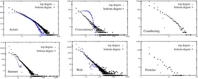
This decomposition scheme gives a bipartite version of any classical network. It is designed to produce (artificial) bipartite networks with the same kind of properties as the natural ones, in order to make them suitable for the modelling issues below. To this respect, it is important that we pick only one clique for each link, since we want the number of top nodes to be in the same order of magnitude as the size of the original network (if we take for example all the maximal cliques but not just one then we can obtain an exponential number of top nodes). Likewise, it is crucial to choose large cliques whenever we can since in real-world bipartite networks, a non-trivial number of large cliques appear. This is why we choosed to take maximal cliques. As shown in Figure 2, the degree distributions of the obtained artificial bipartite networks are very similar to the distributions of the natural bipartite ones: bottom degree distributions fit very well power laws, while top degree distributions are of two kinds, either Poisson shaped or heavy tailed.
This last point indicates that the distribution of cliques sizes (i.e. the top degree distributions) may vary qualitatively between networks. This is true both for natural bipartite networks and for the ones obtained using our decomposition scheme.
bottom degree top degree Actors 1 10 100 1000 10000 100000 1e+06 1 10 100 1000 top degree Cooccurrence bottom degree 1 10 100 1000 10000 1 10 100 1000 10000 top degree bottom degree Coauthoring 1 10 100 1000 10000 1 10 100 top degree bottom degree Internet 1 10 100 1000 10000 100000 1e+06 1 10 100 1000 10000 Web top degree bottom degree 1 10 100 1000 10000 100000 1e+06 1 10 100 1000 10000 top degree bottom degree Proteins 1 10 100 1000 10000 1 10 100
Figure 2: Top and bottom degree distributions for the natural bipartite versions of Ac-tors, Cooccurrence, and Coauthoring, and for the bipartite version of Internet, Web, and
Proteins obtained with the decomposition scheme.
Since all these networks have similar underlying bipartite structure, one may wonder if their properties (like clustering) can be viewed as consequences of this structure. We
explore this idea below.
Two bipartite models.
The first natural way to derive a model from our observations is to sample uniformly random bipartite networks with prescribed (top and bottom) degree distributions. As explained in [26], this can be achieved as follows: first generate both top and bottom nodes
and assign to each a degree drawn from the given distributions1, then create for each node
as many connection-points as its degree, and finally link top and bottom connection-points randomly.
The properties of this random bipartite model are studied in [17, 26], where it is shown, both analytically and empirically, that the obtained networks have the desired properties (mainly high clustering, and power law degree distribution). Therefore, these properties can be viewed as consequences of the underlying bipartite structure.
Notice that the degree of a bottom node is not its degree in the unipartite version of the bipartite network (see for instance Figure 1), but the number of cliques (top nodes) it belongs to (it is linked to). Therefore, it is not trivial that the random bipartite model captures well the original degree distribution. Likewise, the high clustering of the obtained network may be seen as a consequence of the fact that there are cliques of exactly the same sizes (distributed according to the top degree distribution), and it is indeed true. However, it was not clear until now that the presence of cliques is sufficient to capture this, and, more important, no method was known to sample realistic networks with both high clustering and power law degree distribution.
The random bipartite model assumes that two distributions, for both top and bottom degrees, are explicitly given. We can also use the preferential attachment principle to define them implicitly. Indeed, as already noticed, the bottom degree distributions gen-erally follow a power law. This leads to a growing model defined as follows. At each step, a new top node is added and its degree d is sampled from a prescribed (top) distribution (which qualitatively varies between networks). Then, for each of the d links of the new top node, either a new bottom node is added (with probability λ) or we pick one among the preexisting ones using preferential attachment (with probability 1 − λ). The parameter
λ is the overlap ratio, defined as 1 minus the ratio between the number of nodes and the
sum of the sizes of the cliques: λ = 1 − P n
v∈⊤d
o(v). We use it to compute the ratio of new
bottom nodes to which a new top node is connected, which ensures that the obtained network has this overlap ratio. It can be computed both on real-world bipartite networks and on ones obtained using the decomposition scheme, which gives values greater than 0.5 in general (see Table 1).
1Notice that this may lead to incompatible top and bottom degree sequences, in the sense that the
sum of top degrees is different of the sum of bottom degrees. In such a case, one can simply solve the problem by sampling again the degree of a randomly chosen top and bottom node, until the distributions are compatible.
By definition, at each step the bipartite network has the required degree distributions and the same overlap ratio as the original network. Notice that this construction process is very similar to the one observed in some real-world cases. For instance, Actors is built exactly this way: when a new movie is produced (which corresponds to the addition of a top node), it is linked to actors according to their popularity, and to some new actors, playing in a movie for the first time.
Original Rand. bip. Pref. att. Actors 1 10 100 1000 10000 100000 1 10 100 1000 10000 100000 Original Rand. bip. Pref. att. Cooccurence 1 10 100 1000 1 10 100 1000 10000 Rand. bip. Pref. att. Coauthoring Original 1 10 100 1000 10000 1 10 100 1000 Internet Original Pref. att. Rand. bip. 1 10 100 1000 10000 100000 1 10 100 1000 10000 100000 Web Original Rand. bip. Pref. att. 1 10 100 1000 10000 100000 1e+06 1 10 100 1000 10000 100000 Proteins Original Rand. bip. Pref. att. 1 10 100 1000 10000 1 10 100
Figure 3: The original degree distribution of our six examples, together with the ones of the unipartite networks obtained from the random bipartite model and with the prefer-ential attachment bipartite model.
The degree distribution and the clustering of the networks obtained with both models can be compared with the actual networks’ degree distribution and clustering, and with the performances of the main models currently used. This is summarized in Table 1 (clus-tering and other) and in Figure 3 (degree distributions). In several cases, the simulations fit the real-world values surprisingly well. In all the cases, our models give results much more accurate than the commonly used models, considering the all the features together. There are however differences between the values obtained from the bipartite models and the real-world networks. They are consequences of the following fact. In the original bipartite networks (both natural ones and the ones obtained from the decomposition), many top nodes have a large neighborhood intersection. In other words, the overlap between cliques is large, and more precisely, if two cliques have one node in common then they certainely have many. This behavior can be viewed as a kind of bipartite clustering, which is not captured by the bipartite models: the random linking implies that most cliques have only one node in common, if any. This is responsible both for the inaccuracy of the models concerning some clusterings and for the irregularities one can observe on some distributions.
Internet Web Actors Co-auth Co-occur Protein n 75885 325729 392340 16401 9297 2113 m 357317 1090108 15038083 29552 392066 2203 α 2.5 2.3 2.2 2.4 1.8 2.4 nc 269236 565116 127823 19885 13588 1940 λ 0.888 0.833 0.733 0.643 0.949 0.478 C 0.171 0.466 0.785 0.638 0.822 0.153 Crd 0.0001 0.00002 0.0002 0.0002 0.009 0.001 Cdd 0.0694 0.017 0.0057 0.001 0.26 0.007 Cab 0.0024 0.0005 0.0015 0.003 0.028 0 Cws 0.171 0.461 0.74 (*) 0.523 (*) 0.74 (*) 0.06 (*) Crb 0.32 0.663 0.767 0.542 0.831 0.187 Cgb 0.65 0.708 0.793 0.632 0.768 0.244 d 5.80 7 3.6 7.18 2.13 6.74 drd 5.25 5.47 2.97 7.57 2.06 10.4 ddd 3.25 4.48 2.95 5.77 2.36 5.73 dab 4.15 5.1 2.93 5.5 2.38 8.15 dws 5.90 11.23 2559 (*) 2269 (*) 55.6 (*) 509 (*) drb 2.97 3.2 3.06 5.07 2.06 5.8 dgb 2.81 3.53 2.83 3.98 2.6 5.45
Table 1: The main statistics for the complex networks we use in this paper. For each network,
we give its number of vertices n, its number of links m, the value of the exponent α of its power law degree distribution, its clustering coefficient C, and its average distance d. We also give the number of cliques nc in the corresponding decomposiiton, as well as the overlap ratio λ. Moreover, we give the values of these parameters for typical graphs with the same number of vertices and links obtained with commonly used models and the bipartite models: the purely random model [13] (Crdand drd), the random model with prescribed degree distribution [19, 20]
(Cdd and ddd), the Albert and Barab´asi model [3] (Cab and dab), Watts and Strogatz model [31]
(Cws and dws), the random bipartite model with prescribed degree distributions (Crb and drb),
and the growing one with preferential attachment (Cgb and dgb). Notice that purely random
graph and Watts and Strogatz ones have a Poisson degree distribution, which makes the α exponent irrelevant in these cases, and makes them irrelevant for realistic modelling of complex networks. Moreover, in the cases pointed by a star (*), the real clustering coefficient is too large to be obtained with the Watts and Strogatz model. Therefore we used in these cases the parameters inducing the maximal clustering, which yields very large average distances.
For example, in the case of Internet, we noticed the presence of a sub-network of only 94 nodes which contains all the 494 cliques of size 14 and more. This makes this sub-network very dense. On the other hand, in the unipartite versions of random bipartite networks, these large cliques are disseminated all over the network which brings two artifacts: there are a lot of nodes having a degree between 14 and 29 which explains the bump on degree distribution (a similar phenomenon can be observed on Web), and the clustering is drastically increased.
Finally, let us insist on the fact that our aim is to produce networks fitting qualitatively the properties of the original ones, which is achieved in all the cases. Moreover, the results we obtain are much more accurate than the ones obtained with commonly used models.
Conclusion.
In this communication, we proposed a scheme to decompose any complex network into a bipartite one. This allowed us to study and compare the statistics of both natural and artificial bipartite networks, which revealed surprising similarities. In particular, the bottom degree follows a power law, and there are large cliques in real-world networks.
The properties of various complex networks, like clustering and degree distributions, are also properties of unipartite versions of random bipartite networks. Therefore, they can be seen as consequences of a hidden underlying bipartite structure.
This leads us to propose both the random bipartite model and the growing bipartite model with preferential attachment as two general models for complex networks. The choice between these two models depends on one’s aim. For instance, the second should be preferred if the growth of the network is a key issue, whereas the first should be used in situations where one knows exactly the desired degree distributions.
The obtained networks fit very well the properties of real-world networks, using only their general bipartite structure. The bipartite models therefore provide an interesting alternative to those previously proposed. Of course, real-world networks have other prop-erties not captured by the bipartite models (we discussed the case of the overlap between cliques). There is still a lot to do in this direction, and certainely extensions of these models can be defined to improve their accuracy (we currently work in this direction). Acknowlegements.
We thank Cl´emence Magnien and James Martin for careful reading of preliminary versions and useful comments. We also thank the anonymous referees for their help in improving the manuscript.
References
[1] R. Albert and A.-L. Barab´asi. Emergence of scaling in random networks. Science, 286:509– 512, 1999.
[2] R. Albert and A.-L. Barab´asi. Statistical mechanics of complex networks. Reviews of Modern Physics 74, 47, 2002.
[3] R. Albert, H. Jeong, and A.-L. Barab´asi. Diameter of the world wide web. Nature, 401:130– 131, 1999.
[4] R. Albert, H. Jeong, and A.-L. Barab´asi. Error and attack tolerance in complex networks. Nature, 406:378–382, 2000.
[5] arXiv.org e Print archive. http://arxiv.org/.
[6] A.-L. Barab´asi. Linked: The New Science of Networks. Perseus Publishing, 2002. [7] B. Bollob´as. Random Graphs. Academic Press, 1985.
[8] S. Bornholdt and H.G. Schuster, editors. Handbook of Graphs and Networks. Wiley-VCH, 2003.
[9] Self-Organized Networks Database. http://www.nd.edu/~networks/database/index.html. [10] The Internet Movie Database. http://www.imdb.com/.
[11] S.N. Dorogovtsev and J.F.F. Mendes. Evolution of networks. Adv. Phys. 51, 1079-1187, 2002.
[12] S.N. Dorogovtsev, J.F.F. Mendes, and A. Samukhin. Structure of growing networks with preferential linking. Phys. Rev. Lett. 85, pages 4633–4636, 2000.
[13] P. Erd¨os and A. R´enyi. On random graphs I. Publ. Math. Debrecen, 6:290–297, 1959. [14] R. Ferrer and R.V. Sol´e. The small-world of human language. In Proceedings of the Royal
Society of London, volume B268, pages 2261–2265, 2001.
[15] Internet Maps from Mercator. http://www.isi.edu/div7/scan/mercator/maps.html. [16] R. Govindan and H. Tangmunarunkit. Heuristics for internet map discovery. In IEEE
INFOCOM 2000, pages 1371–1380, Tel Aviv, Israel, March 2000. IEEE.
[17] J.-L. Guillaume and M. Latapy. A realistic model for complex networks. 2003. cond-mat/0307095.
[18] H. Jeong, B. Tombor, R. Albert, Z. Oltvai, and A.-L. Barab´asi. The large-scale organization of metabolic networks. Nature, 407, 651, 2000.
[19] M. Molloy and B. Reed. A critical point for random graphs with a given degree sequence. Random Structures and Algorithms, pages 161–179, 1995.
[20] M. Molloy and B. Reed. The size of the giant component of a random graph with a given degree sequence. Combin. Probab. Comput., pages 295–305, 1998.
[21] C. Moore and M.E.J. Newman. Epidemics and percolation in small-worlds networks. Phys. Rev. E, 61:5678–5682, 2000.
[22] M.E.J. Newman. Scientific collaboration networks: I. Network construction and fundamen-tal results. Phys. Rev. E, 64, 2001.
[23] M.E.J. Newman. Scientific collaboration networks: II. Shortest paths, weighted networks, and centrality. Phys. Rev. E, 64, 2001.
[24] M.E.J. Newman. The spread of epidemic disease on networks. Phys. Rev. E, 66, 2002. [25] M.E.J. Newman. The structure and function of complex networks. SIAM Review, 45(2):167–
256, 2003.
[26] M.E.J. Newman, D.J. Watts, and S.H. Strogatz. Random graph models of social networks. Proc. Natl. Acad. Sci. USA, 99 (Suppl. 1):2566–2572, 2002.
[27] R. Pastor-Satorras and A. Vespignani. Epidemic spreading in scale-free networks. Phys. Rev. Lett., 86:3200–3203, 2001.
[28] R. Pastor-Satorras and A. Vespignani. Evolution and Structure of the Internet: A Statistical Physics Approach. Cambridge University Press, 2003. To appear.
[29] S.H. Strogatz. Exploring complex networks. Nature 410, March 2001. [30] Bible Today New International Version. http://www.tniv.info/bible/.
[31] D.J. Watts and S.H. Strogatz. Collective dynamics of small-world networks. Nature, 393:440–442, 1998.