HAL Id: hal-02393818
https://hal-univ-rennes1.archives-ouvertes.fr/hal-02393818
Submitted on 12 Feb 2020HAL is a multi-disciplinary open access archive for the deposit and dissemination of sci-entific research documents, whether they are pub-lished or not. The documents may come from teaching and research institutions in France or
L’archive ouverte pluridisciplinaire HAL, est destinée au dépôt et à la diffusion de documents scientifiques de niveau recherche, publiés ou non, émanant des établissements d’enseignement et de recherche français ou étrangers, des laboratoires
Patient-specific and real-time model of numerical
simulation of the hemodynamics of type B aortic
dissections
J Tomasi, F Le Bars, C Shao, A Lucas, M Lederlin, P Haigron, J P Verhoye
To cite this version:
J Tomasi, F Le Bars, C Shao, A Lucas, M Lederlin, et al.. Patient-specific and real-time model of numerical simulation of the hemodynamics of type B aortic dissections. Medical Hypotheses, Elsevier, 2020, 135, pp.109477. �10.1016/j.mehy.2019.109477�. �hal-02393818�
Patient-specific and real-time model of numerical simulation
of the hemodynamics of type B aortic dissections
J. TOMASI, MD 1, F. LE BARS, MD 1, C. SHAO 2, A. LUCAS, MD 3, M. LEDERLIN, MD, PhD 4,
P. HAIGRON, PhD 5, J.P. VERHOYE, MD, PhD 1
1 Service de Chirurgie Thoracique et Cardiovasculaire, CHU Pontchaillou, Rennes, France
2 Ansys Inc., Villeurbanne, France
3 Service de Chirurgie Vasculaire, CHU Pontchaillou, Rennes, France
4 Service de Radiologie, CHU Pontchaillou, Rennes, France
5 Laboratoire Traitement du Signal et de L’image (LTSI), INSERM 1099U, Université Rennes 1,
Rennes, France
Corresponding author
Name: Florent LE BARS, MD Address: CHU Pontchaillou
2 rue Henri Le Guilloux 35 000 RENNES FRANCE E-mail: Florent.LE.BARS@chu-rennes.fr Phone: 00 33 2 99 28 57 65 Fax: 00 33 2 99 28 24 96 Funding
The authors received no specific funding for this work, but it was made in partnership with Ansys Inc.
PREAMBLE
This scientific research work is the fruit of the participation of a multidisciplinary team,
involving doctors, researchers and engineers, confirmed and in the course of formation, within
an association between the LTSI * and the Ansys Inc.**.
From this article follows the realization of a science thesis of a Doctor of Medicine, a
doctorate of an engineer and a Master of Science of another Doctor of Medicine.
The role of the engineer consisted in the creation of the simulation model and the
optimization of this one, whereas the role of the doctors of medicine was to allow a clinical
coherence of the model during its development, to set up the clinical research allowing the
acquisition and the collection of the medical data and the parameterization of the final model
in order to recreate coherent clinical situations in simulation.
* Laboratoire Traitement du Signal et de l’Image, is an INSERM unit (Institut National de la
Santé et de la Recherche Médicale), working in close collaboration with the University Hospital
of Rennes on numerous medical research projects involving technologies and engineering
sciences.
ABSTRACT
Introduction: Regular monitoring of uncomplicated type B aortic dissection is essential
because 25 to 30% will progress to aneurysmal form. The predictive factors of this evolution
are not clearly defined, but they seem to be correlated with hemodynamic data.
Hypothesis: Our goal is to create a patient-specific and real-time model of numerical
simulation of the hemodynamics of uncomplicated type B aortic dissections in order to predict
the evolution of these pathologies for earlier treatment.
Method: This model consists in a coupling 0D (hydraulic-electric analogy) - 3D (CT angiography
segmentation) of the aortic arch with optimization by comparison to the 2D Phase Contrast
MRI data and using Reduced Order Models to drastically reduce computing times. We tested
our model on a healthy and a dissected patient. Then we realized different systolic blood
pressure scenarios for each case, which we compared.
Results: In the dissected patient, the blood pressure at the false lumen wall was less important
than the true lumen. Furthermore, the aortic wall shear stress and the velocity fields in aorta
increase at the entry and re-entry tears between the two lumens. The simulation of different
blood pressures scenarios shows a decrease in all these three parameters related to the
decrease of the systolic blood pressure.
Conclusion: Our model provides reliable patient-specific and real-time 3D rendering. It has
also allowed us to realize different flow variation scenarios to simulate different clinical
conditions and to compare them. However, the model still needs improvement in view of a
INTRODUCTION
Aortic dissection is a rare (3.2 / 100,000 inhab. /year) but serious disease (50% of mortality
at 48 hours and 90% at 3 months), which realizes a cleavage within the aortic wall what
creating a false lumen that may be responsible for aortic rupture and / or organ perfusion at
the acute phase.
We distinguish the forms interesting the ascending aorta (type A dissection), where the
risk of intra-pericardial rupture is high and for which urgent surgical management by
replacement of the ascending aorta is the reference, and type B dissections which by
definition does not interest the ascending aorta.
Currently, for the initial management of these type B aortic dissections, the decision tree
is as follows:
- Uncomplicated dissections (i.e. without signs of rupture or mal-perfusion) should benefit
from optimal medical treatment by blood pressure (BP) monitoring (systolic BP <120mmHg)
and active medical supervision.
- Complicated dissections should be surgically treated, for which Thoracic EndoVascular
Aortic Replacement (TEVAR) become the gold standard when anatomical conditions are
favorable (1).
Two essential evolutionary phases of these initially uncomplicated dissections must be
distinguished. The first is the acute phase between 0 and 30 days with a risk of mal-perfusion
and rupture for which surgical intervention is associated in 24%. The second is the chronic
phase where 25 to 30% will evolve to aneurysmal form or secondary mal-perfusions at 4 years
The current clinical problem is: Whose propose an early endovascular procedure in
uncomplicated situation to prevent chronic complications?
Existing anatomical elements that have been identified as predictors of poor long-term
outcome in type B dissections, such as an initial aortic diameter over 40 mm in the acute
phase, a false lumen over 22 mm of diameter, an elliptical true lumen and a circular false
lumen and an entry tear located less than 5 centimeters from the origin of the left subclavian
artery (3). But these are not enough to initiate a surgical management. The definition of this
sub-population concerned is therefore still debated.
A better understanding of hemodynamic events such as comprehension of pressure
regimes between the true and the false lumen, wall shear stress and blood velocities fields
can help to refine this complex hemodynamics. Some of these data are accessible through
medical imaging such as aortic geometry by CT or flow data by MRI. However, no examination
can quantify the pressure and the shear stress that apply to the aortic wall, as well as the
blood velocity fields. These data are therefore only accessible through computerized
simulation models (Computational Fluid Dynamics (CFD)) that are currently rarely
HYPOTHESIS / GLOBAL PROBLEM
The hypothesis of our work is to know if it is possible to predict the evolution of
uncomplicated type B aortic dissections in time through numerical simulation of
hemodynamics and this specifically for each patient.
One of the main challenges is to have shorter simulation times than real life so that the
simulation tool can have a clinical interest. The ultimate interest is to determine profiles of
patients at risk for chronic complications of their dissection and for whom earlier surgical
management would avoid these complications.
INITIAL PROBLEM
The first step of the work consists in the realization of the patient-specific and real-time
computer model, allowing the simulation of flow variations in the aortic arch in a healthy
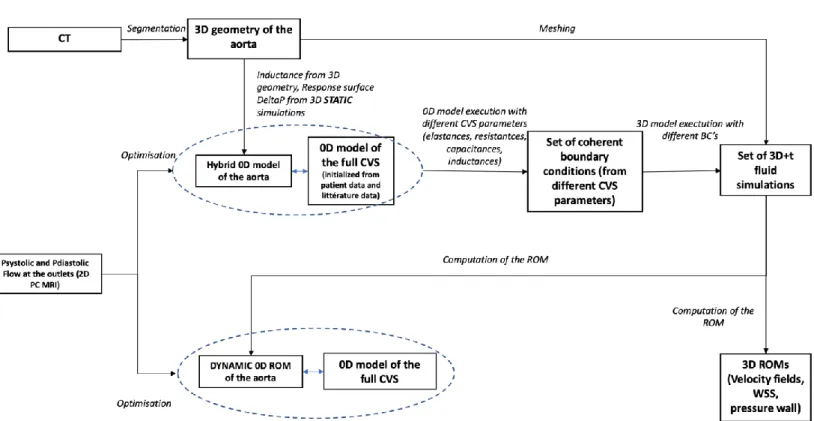
HYPOTHESIS ASSESMENT (Figure 1) Clinical data management
For the realization of our work we needed a healthy subject to create the healthy aorta
model and a subject with uncomplicated type B aortic dissection to test the model. The
healthy subject was included on the basis of volunteering and dissected subject was included
prospectively in the acute phase of his pathology after information, written and oral, clear,
fair and appropriate and not opposed from him to participate at the study. For both, the only
inclusion criterion was to be major and the exclusion criteria were having a pathological aorta
for the healthy subject, having aortic dissection of type A or type B complicated for the
dissected subject, and present a contraindication to performing an MRI for both groups.
Clinical data such as sex, age, heart rate, blood pressure and treatments were also
collected.
To carry out this study, we had the agreement of the patient protection committee
through the protocol “hors loi Jardé” because it involves the human person but does not
belong to an interventional study since the MRI is a common follow-up exam of the aortic
dissections.
Choice of 0D mode
To reduce computational time and make the model usable in clinical practice, we used
aortic arch model reduction using a 0D-3D coupled model to provide the boundary conditions
for the aortic arch 3D simulation. This 0D model is based on the concept of hydraulic-electrical
analogy: blood flow equivalent to an electrical current, blood pressure between two points to
a voltage, vessel elasticity to a capacitance (C), vascular resistances to a resistance (R) and
physiological variables of interest (e.g. pressure, flow and volumes) are uniformly distributed
in space. This model works in a closed-loop to get as close as possible to the full cardiovascular
system (CVS) with its three compartments, which are the systemic circulation, the pulmonary
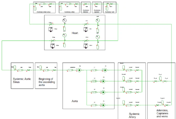
circulation and the heart. After a review of the literature we chose the 0D model of
Korakianitis et al. (4) because it is a simple model that represents the full CVS in the form of
closed loop while integrating various vascular segments of interest (coronary sinuses, arteries,
arterioles, capillary, veins). We then reproduced it on the Twin Builder software (Ansys,
Canonsburg, Pennsylvania, USA) (Figure 2).
3D geometrical modeling of the aorta
In our work we included two patients, one with healthy aorta and one with dissected aorta
(uncomplicated type B dissection starting just after the ostium of the left subclavian artery at
the outer aortic arch curvature) having already been operated several years ago on a
mechanical Bentall procedure (replacement of the aortic valve with a mechanical prosthesis
and of the initial part of the aorta with a synthetic tube) for aortic root aneurysm with aortic
valve regurgitation.
In these two patients we performed a chest CT scan, at low X-ray dose and without
contrast injection for the patient with healthy aorta and normal X-ray dose and contrast
injection for the dissected patient. These scanners made it possible to perform aortic
segmentation, using 3DSlicer software (open source software), to obtain the 3D geometric
models of these aortas (Figure 3). At the same time, we realized a 2D Phase Contrast (PC) MRI,
to obtain noninvasively the hemodynamic data that will serve as a reference for the
For a sake of simplicity to create our model, we were interested only at the hemodynamic
study of the aortic arch and the first centimeters of the descending thoracic aorta
(abandonment of the ascending aorta (AA) because it does not correspond to the definition
of dissection of type B). This gives us a system with one inlet (initial part of the arch) and four
outlets (brachiocephalic trunk (BT), left common carotid artery (LCC), left subclavian artery
(LS) and descending thoracic aorta (DA)) for the healthy patient and five outlets (BT, LCC, LS,
true and false lumen (TL and FL)) for the dissected patient. Dissected patient to whom we also
found two entries tears of the dissection just after the ostium of the LS, and two re-entries in
the DA.
0D Model modification
The direct coupling between the 0D model of the full CVS and the 3D aortic geometry is
complicated because the values of the 0D model parameters of the CVS are not available in
the literature. This step is essential because a wrong calibration of its parameters can lead to
a problem of correlation of the output of the 3D model of the stick which produces numerical
instabilities.
To circumvent this problem, an equivalent 0D model of aortic arch was created, based on
static simulations (absence of the time effect, open circuit) and electric model (inductance) to
have an approximation of the 3D transient fluid simulation of the arch and for secondarily be
coupled to the 0D model of the full CVS. Then this model allowed us to obtain pressure and
flow curves that served us as boundary conditions for our 3D simulation.
3D models are based on the resolution of Navier-Stokes equations, applied to the finite
element discretization of the 3D model. The 3D model of aortic arch was divided into five or
segment of the aortic arch was represented using an inductance and a pressure source whose
values are derived from static simulations. In our models we make the assumption that the
wall is rigid, so we did not use capacitance. For the representation of the wall of the aortic
arch the 3D volume consisted of a polyhedral mesh and eight prism layers, for the blood a
Newtonian incompressible fluid model was used and for the model of turbulence the model
SST k- ω.
For the computation of the pressures, the static simulation consists of applying an inlet
pressure (Pinlet) at the ascending aorta and flow rates at each outlet (Qoutlet) in order to
determine the outlet pressures (Poutlet). For this we did this simulation many times by varying
the values of Pinlet and Qoutlet applied. We have recovered at each calculation calculated
Poutlet (static ROM). From the results, we used a response surface which made it possible to
reduce the calculation times. This makes it possible to obtain instantaneously the values of
the pressure sources for each set of boundary conditions. For the calculation of the inductance
parameter in each branch, we used the geometrical values of each branch (radius and length)
assuming it was a perfect cylinder and we applied the Poiseuille law (Figure 4).
Then, the 0D model based on static simulations of the aortic arch was coupled to the full
CVS model. The three upper outlets were connected to a block consisting of resistance,
capacitance and inductance to represent the systemic arterioles, capillaries and veins of the
upper body. The two lower outlets were connected to the same block type to represent the
systemic part of the lower body. The fact to having capacitances in the full CVS model makes
it possible to simulate the compliance of the vessels. As a result, in our full CVS model, only
The integration of the static model of the aortic arch with the 0D model of the full CVS
allowed us at this stage to have a full CVS 0D model with the representation of the aortic arch
(Figure 5).
Personalization of the 0D Model using the 2D PC MRI Flow Data
Once the basic model 0D with integration of the aortic arch was realized, it remained to
calibrate it to make it patient-specific. The adjusted parameters were the resistance,
capacitance, and inductance values of the systemic part of the model, as well as the atrial and
ventricular elastance parameters. The aim was to correlate the flows at the outlet calculated
from the 0D model (flow / pressure curves - Dynarom) to the flows obtained from the patient's
2D PC MRI data, which serve as objective references. And this throughout the cardiac cycle, in
systole and diastole.
For this we used the Levenberg-Marquardt optimization method to optimize the model
(5). This method solves non-linear least squares problems and has shown good performance
in minimizing least-squares curve fitting.
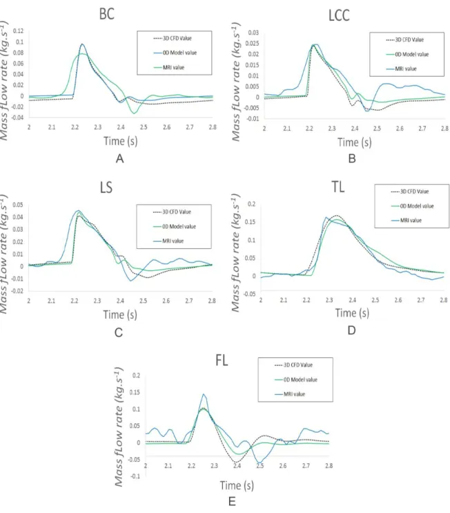
As a result of the optimization, the flows rates at the outlet of the 3D transient fluid
simulations and the 0D model of the full CVS were very close, particularly in the systolic phase.
Note that the reverse flow phenomenon is underestimated with the 0D model for all outputs,
except for true light. (Figure 6).
0D model simulation results (flow / pressure curves)
Once the 0D model was set up, we performed the simulations using the Twin Builder
software to obtain the results of the simulation in the form of flow and pressure curves
Attribution of the 0D model’s boundary conditions
However, all the difficulty in this 0D model was the attribution of the boundary conditions
so that the results from the 3D transient fluid simulation were clinically plausible. We
performed several calculations with different boundary conditions to obtain multiple results
in order to create a Reduced-Order Modeling (ROM). As a reminder, a ROM aims to reduce
the complexity of mathematical calculations by reducing the size of the space or the degrees
of freedom to obtain an approximation of the original model. The ROM requires an important
learning set, hence the interest to having a wide range of variation between the different
boundary conditions obtained. Value ranges are then assigned for the input flow and the
outputs pressures (e.g. PAs [80; 180 mmHg]).
We also varied the parameters of the 0D models (resistances, capacitances, inductance
and elastance) to obtain different ranges of values for the input flow and the pressure. For
each set of boundary conditions, we performed a 3D transient fluid simulation for which the
computation time is approximately 24 hours for 3 cardiac cycles.
Integration of data from the 0D model and 3D representation
To obtain the images of the simulation, at each calculation, we saved the values that
interested us at each time step chosen. In our study we are interested only in the peak systole
to study the part of the cardiac cycle where the blood pressure is the most important. On the
other hand, for ROM and 3D calculations we took into account the whole cardiac cycle.
From these results we could create ROMs. Our ROM model consists of nonlinear
differential equations that connect the solver inputs to the solver outputs using neural
At this stage of our work we use two different types of ROMs: one calculates the transient
results of aortic flow and pressure to replace the static model (dynamic ROM) and the other
calculates the 3D physical variables (dynamic ROMs) which provides 3D values of the aortic
arch for each of the hemodynamic data of interest (x3): wall shear stress, wall pressure and
blood velocity field.
The results obtained from the 3D dynamic ROM simulation were then transmitted to the
CFD-Post software (Ansys) to obtain the 3D representations and make comparisons between
the different scenarios (Figure 8).
Model optimization
Once the aortic arch dynamic ROM was functional, it replaced the initial static 0D model
of the aortic arch (static simulations of pressures and inertances) to obtain a 0D dynamic ROM
model of the aortic arch.
Parameters of the 0D model (dynamic this time) were optimized by a new confrontation
with the 2D PC MRI data to match to the clinical data of the patient at rest.
The comparison between our final 0D dynamic ROM model and the 3D transient fluid
simulation shows a relative difference on average 1.55% and an absolute maximum difference
of 4.26mmHg for all cumulative Poutlets for the healthy patient. For the dissected patient,
these values are 0.61% and 3.66mmHg respectively. Knowing that the computation time of
the 3D transient fluid simulations is on average 17 hours for the healthy patient and 23 hours
for the dissected patient, while the 0D dynamic ROM model only takes a few seconds for both
Use in a clinical situation
Now we have a final 0D model with integration of the aortic arch for a healthy patient and
for a dissected patient (model 0D dynamic ROM of the arc and model 0D full CVS) (Figure 9).
This allows us to perform different flow simulations by modifying certain parameters, such as
heart rate, to simulate certain real-life situations (stress, stress) or the effects of a medication
(antihypertensive, bradycardic) and obtain hemodynamic data from the aortic arch in real
time.
EMPIRICAL DATA
In our research, we had two patients, one with a healthy aorta and the other with a
dissected aorta, with whom we wanted to simulate different scenarios of BP variations in
order to test our model and then be able to consider different scenarios of prediction of
evolution of type B aortic dissection as a function of adherence to medical treatment.
For the healthy patient with controlled systolic BP (sBP) (i.e. sBP <120 mmHg) measured
at 115 mmHg and diastolic BP (dBP) at 75 mmHg on 2D PC MRI, we simulated high blood
pressure (HBP) (i.e. sBP > 140 mmHg).
For the dissected patient with moderately controlled sBP (i.e. sBP between 120 and 140
mmHg) measured at 135 mmHg and dBP at 73 mmHg on 2D PC MRI, we used two scenarios
of sBP. A reduction to obtain a controlled sBP (i.e. <120 mmHg) and an increase to obtain an
uncontrolled sBP (i.e. > 140 mmHg).
As a reminder, in the case of aortic dissections, the blood pressure objective is less than
Healthy patient case "High pressure" scenario
To simulate the "high pressure" scenario, we chose to simulate vasoconstriction by
increasing vascular resistance (venous) without changing the cardiac frequency (CF).
Before simulation and according to the MRI data the healthy patient had a systolic ejection
volume (SEV) at 93 ml and a CF at 66 bpm, which by the relation Q = SEV x CF gave a cardiac
flow (Q) at 6.1 L / min and a Q peak at 0.45 L / sec.
After simulation through our 0D model we achieved HBP with a sBP at 145 mmHg with an
increase of dBP at 115 mmHg but a decrease of Q peak at 0.38L / sec.
Healthy patient simulations
A comparison of the aortic wall pressure shows a greater wall pressure in the "high
pressure" scenario. It is also noted that the blood flow is laminar in both cases since there is
very little pressure wall variation (Figure 10).
The comparison of the aortic wall shear stress shows more stress zones at the level of the
Supra-Aortic Trunks (SAT) but not at the level of the aorta. The analysis of the differences
between the two models shows a very small difference in the order of less than 20 Pa / 0,15
mmHg in favor of greater stress for the healthy patient with "controlled pressure" scenario
(Figure 11).
The comparison of the aortic blood velocities fields shows accelerations at the level of the
SAT and at the outer curvature of the initial part of the aortic arch. The analysis of the
differences between the two models shows a very small difference of the order of less than
Dissected patient case
"Controlled pressure" scenario
To simulate the "controlled pressure" scenario, we chose to simulate beta-blocker
antihypertensive drug use as it is the main antihypertensive drug used in aortic dissection. The
action of beta-blockers is primarily at the cardiac level by reducing heart rate, cardiac
excitability and myocardial contractibility. So, we focused on acting on these parameters
through our model, to reduce cardiac output. Based on the patient's MRI data, the patient
had a SEV at 69 ml, a CF at 76 bpm, a Q at 5.3 L / min and a Q peak at 0.38L / sec. We therefore
first directly decreased the heart rate at 60 bpm in the parameters of our model and secondly
divided by 8.33 the initially defined parameters of elastance of the left atrium and the left
ventricle to have a SEV equivalent to 69ml. With these two modifications we obtained through
the 0D simulation a Q at 4.1 L / min (69 x60 / 1000) with a Q peak at 0.31 L / sec, a sBP peak
at 112 mmHg and a dBP peak at 55 mmHg.
"High pressure" scenario
To simulate the "high pressure" scenario we had several physiological possibilities of BP
increase. We chose to vary the responsible factors of chronic HBP, either arterial resistance
simulating vasoconstriction or venous capacitance simulating hypervolemia (7).
First, note that the sum of systemic vascular resistance in our 0D model for the dissected
reference patient is 82 MPa.s / m3 for normal values from the literature (6) between 70 and
160 MPa.s / m3 reinforcing the accuracy of our model. Moreover, in our 0D model, for the
reference dissected patient the arterial resistances of the FL are less important than those of
In both "vasoconstriction" and "hypervolemia" scenarios we were able to obtain the same
sBP values of 165 mmHg, either by increasing the arterial resistances 6.5 times, or by
increasing the venous capacitance 2.5 times. On the other hand, the values of dBP and Q
differed. In the "vasoconstriction" scenario, the dBP was 92 mmHg and the Q peak was stable
at 0.37 L / sec for a stable Q as well. In the "hypervolemia" scenario, the dBP was 88 mmHg,
whereas the Q peak was increased to 0.47 L / sec, indicating an increase in Q.
Dissected patient simulations
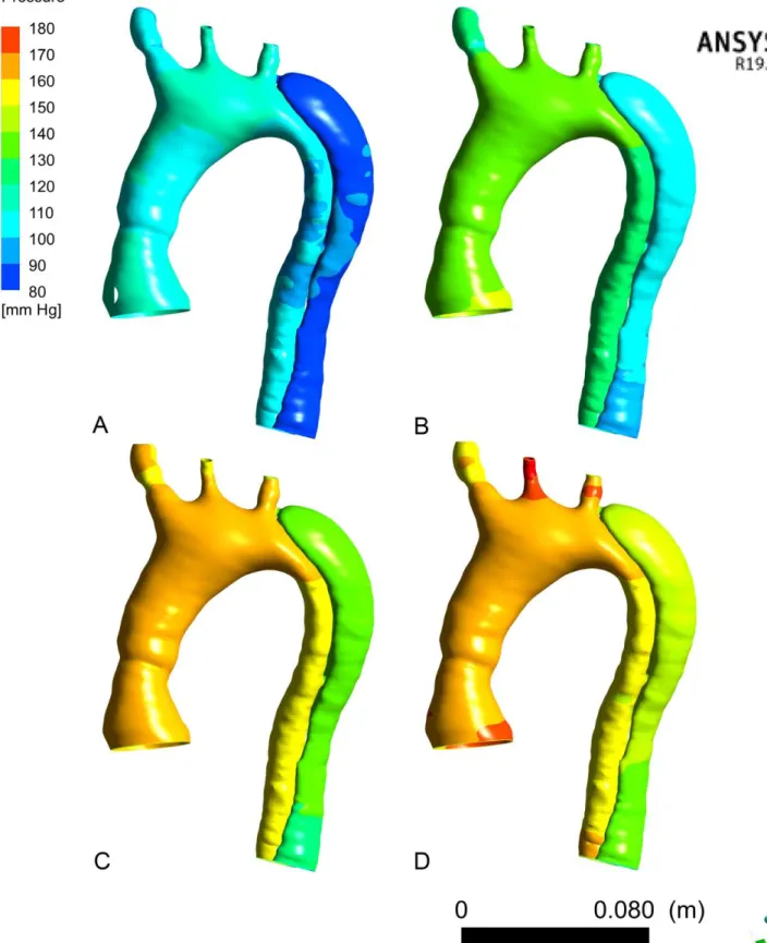
The comparison of the aortic wall pressures of the 4 scenarios applied shows for each of
the scenarios a lesser pressure at the FL wall (approximately 30mmHg) (Figure 13). As for the
TL, the wall pressure of the FL also increases with the increase of sBP. For the last two
scenarios (Figure 13 C and D) the pressure in the arch and the TL is broadly similar, however
the Q peak causes a slight increase of the pressure wall of the FL for the scenario "high
pressure by hypervolemia" (Figure 13 D).
The comparison of the aortic wall shear stress of the 4 scenarios applied shows for each
of the scenarios, zones of greater wall shear stress at the level of the suture zone of the
ascending aorta, at the two entries tears of the dissection after the ostium of the left
subclavian artery, at the two re-entries tears in the descending thoracic aorta and at the aortic
wall of the FL in front these four communications (Figure 14). It is also noted that these wall
shear stress increase at these locations with increasing sBP. As for wall pressures, the wall
shear stress at the aortic wall are increased in the "high pressure by hypervolemia" scenario
(Figure 14 D) where the Q peak is higher.
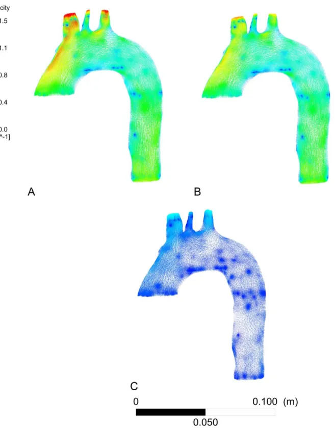
The comparison of aortic blood velocities fields of the 4 scenarios shows for each of the
aorta, at the two entries tears of dissection after leaving the ostium of the left subclavian
artery and the two re-entries in the descending thoracic aorta (Figure 15). We also note that
these speeds increase at these locations with the increase in sBP. As with wall pressures and
wall shear stress, blood velocities in the aorta are increased in the "high pressure by
hypervolemia" scenario (Figure 15 D) where the Q peak is higher.
DISCUSSION Results interpretation
The analysis between the two scenarios in the healthy patient, shows a very small
difference in values, of the order of less than 20 Pa / 0,15 mmHg for wall shear stress and less
than 0.5 m / sec for blood velocities, favor of the "controlled pressure" scenario. This is
explained by the fact that the Q peak of the patient "controlled pressure" is greater (0.45 vs
0.38 L / sec). This notion shows the interest of decreasing sBP but also Q in the management
of patients in the context of cardiovascular prevention (role of betablockers).
In the dissected patient, analysis of the results showed a decrease of wall pressure in the
FL and a decrease of wall shear stress and blood velocities at the level of communications
between the two lumens related to the decrease in sBP. This confirms the interest of a
reduction of sBP in the management of aortic dissections to limit the extension of the FL and
its rupture in the acute phase and allow its healing and to limit the risk of aneurysmal evolution
(main complication of aortic type B dissections in long-term) (8,9).
We also note that vascular sutures disrupt vessel architecture and hemodynamics, making
State of art
The first step in our work through this article is a feasibility study of our patient-specific
and real-time fluid model of numerical simulation. The findings found are similar to other
studies simulating aortic flow by fluid mechanics in uncomplicated type B aortic dissections
(10-15). They also find an increase of wall shear stress at the entries and re-entries associated
with an increase in velocity fields at the same level. This confirms the good functioning of our
model. On the other hand, these models only transcribe numerically the clinical data of these
patients and do not allow the modification of characteristics such as BP or Q to simulate other
hemodynamic conditions.
Alimohammadi et al. (14) and Dillon-Murphy et al. (15) also integrate a 0D model but use
a Windkessel 0D model which is an open model unlike our closed loop of the full CVS model
which allows us a more precise description of the blood circulation, and therefore to make
different scenarios by varying the parameters, which is much more restricted with a
Windkessel model because of the absence of compartmentalization of the systemic
circulation.
Moreover, thanks to the use of the ROMs we can obtain the results in real time contrary
to the 3D transient fluid simulations (24h for 3 cardiac cycles).
At this stage of our work the originality of our model resides in the way whose is obtained
our model of simulation through a full CVS 0D model and ROM, offering multiple technical and
Advantage of 0D models (full CVS, static arch + inductance)
As previously stated, our 0D model is closed (full body) which allows to have a correlation
between the inlet and outlet and thus a better numerical stability, allowing the realization of
different scenarios.
Moreover, the model integrates many compartments (heart, aortic arch, capillary
arterioles, veins, ...), this allows to simulate different clinical scenarios by varying the
parameters of the model and at different levels.
As for him, the model 0D static + inductance of the arch, makes it possible to avoid directly
coupling of the full CVS 0D model with the 3D model and to obtain pressure and velocity
curves for the 3D computation which is more stable numerically for the calculation.
ROM innovations
The ROM allows to have an instant and realistic representation of the aortic arch in the 0D
dynamic ROM model. This makes the optimization process possible since the number of
calculations is important.
The ROM also allows to have 3D results for any setting of the 0D system and this very
quickly (few seconds).
Advantage of our models
The advantages of any numerical flow simulation reside in obtaining hemodynamic data
in a non-invasive way for patients and at lower cost.
The advantage of the ROM compared to the 3D transient fluid simulation is that the
less than 2% (1.55% and 0.61%). This temporal advantage (real-time) makes it possible to
envisage a daily clinical application which was until now impossible.
Due to the use of CT images for the 3D geometrical representation of aortas coupled with
hemodynamic data by the realization of a 2D PC MRI, we were able to create a patient specific
simulation model, which allows have applicable results to each patient in the daily clinic.
The advantage of the 0D model is that it makes it possible to interact with the various
characteristics of the model in order to vary different values such as CF, Q and / or BP and
thus perform 3D flow simulations that are not derived from the measurements of the MRI
data of the patient but derived from hypothetical scenarios while remaining patient specific.
Limitations
There are several limits to our work. Firstly, we have been limited to the study of the aortic
arch and not to the entire aorta for reasons of simplicity of the model. We have imposed to
the ROM of the aortic arch a rigid and not compliant wall (unlike the rest of the 0D model of
the full CVS) in order to make fewer complex calculations. We have only confronted our model
to one healthy patient and one dissected patient. To obtain the ROMs that allow
instantaneous results, it is necessary first to have made several 3D fluid calculations, which
takes time (about 24 hours). The use of a 4D PC MRI would allow a better confrontation of the
results obtained. There is also a bias that emerges from the fact that the dissected patient has
already undergone cardiac surgery of the aortic valve and the initial segment of the ascending
aorta, which can disturb the hemodynamics at the exit of the heart.
As this work is still in the research phase, several steps are not yet optimized for an instant
clinical application. It requires four different computing platforms and manual controls (0D
Expected improvements
This work presented being that the first part of a research work more consequent, the
model is destined to evolve. The first step will be to create a model of full aorta, from the
aortic sinus to the iliac arteries with integration of a compliant wall of this aorta.
The second step will be the integration of a fatigue model of the aortic wall to simulate
several days or months of cardiac cycles to obtain a predictive model of evolution of the aortic
dissections specific to each patient. The difficulty is to obtain less computation time than the
real time. This would determine the patients most at risk of developing aneurysms and
progression of dissections. The goal is to provide earlier treatment of uncomplicated type B
aortic dissections.
CONCLUSION
The use of the 0D model and ROMs enables a reliable patient-specific and real-time
numerical simulation of the hemodynamics of uncomplicated type B aortic dissections,
opening the doors to clinical use. They also allow simulations in different flow conditions,
which allowed us to confirm the interest of blood pressure reduction in the treatment of aortic
dissections. Being at the beginning of our research, the model is destined to evolve, the goal
is to predict the long-term evolution of aortic dissections and to offer earlier treatment to
REFERENCES
1. Olsson C, Thelin S, Ståhle E, Ekbom A, Granath F. Thoracic aortic aneurysm and dissection:
increasing prevalence and improved outcomes reported in a nationwide population-based
study of more than 14,000 cases from 1987 to 2002. Circulation. 12 déc
2006;114(24):2611‑8.
2. Weiss G, Wolner I, Folkmann S, Sodeck G, Schmidli J, Grabenwöger M, et al. The location
of the primary entry tear in acute type B aortic dissection affects early outcome. Eur J
Cardiothorac Surg. sept 2012;42(3):571‑6.
3. Booher AM, Isselbacher EM, Nienaber CA, Trimarchi S, Evangelista A, Montgomery DG, et
al.The IRAD classification system for characterizing survival after aortic dissection. Am J
Med. août 2013;126(8):730.e19-24.
4. Korakianitis T, Shi Y. A concentrated parameter model for the human cardiovascular
system including heart valve dynamics and atrioventricular interaction. Medical
Engineering & Physics 28.7 (sept. 2006).
p. 613-628, ISSN : 1350-4533, DOI : 10.1016/j.medengphy.2005.10.004.
5. Gavin HP. The Levenberg-Marquardt method for nonlinear least squares curve-fitting
problems. In 2013.
6. Washington University School of Medecine Department of Surgery. Klingensmith, Mary E.
Li Ern Chen; Sean C Glasgow (2008).
7. G. D. Fink, « Sympathetic Activity, Vascular Capacitance and Long-Term Regulation of
Arterial Pressure », Hypertension, vol. 53, no 2, p. 307-312, févr. 2009.
8. Editor’s Choice – Management of Descending Thoracic Aorta Diseases - European Journal
9. Erbel R, Aboyans V, Boileau C, Bossone E, Bartolomeo RD, Eggebrecht H, et al. 2014 ESC
Guidelines on the diagnosis and treatment of aortic diseasesDocument covering acute and
chronic aortic diseases of the thoracic and abdominal aorta of the adultThe Task Force for
the Diagnosis and Treatment of Aortic Diseases of the European Society of Cardiology
(ESC). Eur Heart J. 2014 Nov 1;35(41):2873–926.
10. Shang EK, Nathan DP, Fairman RM, Bavaria JE, Gorman RC, Gorman JH, et al. Use of
computational fluid dynamics studies in predicting aneurysmal degeneration of acute type
B aortic dissections. Journal of Vascular Surgery. 2015 Aug;62(2):279–84.
11. Cheng Z, Tan FP, Riga CV, Bicknell CD, Hamady MS, Gibbs RG, et al. Analysis of flow patterns
in a patient-specific aortic dissection model. J Biomech Eng 2010;132:051007.
12. Karmonik C, Partovi S, Muller-Eschner M, Bismuth J, Davies MG, Shah DJ, et al.
Longitudinal computational fluid dynamics study of aneurysmal dilatation in chronic
DeBakey type III aortic dissection. J Vasc Surg 2012;56:260-3.
13. Cheng Z, Riga C, Chan J, Hamady M, Wood NB, Chesire JW, et al. Initial findings and
potential applicability of computational simulation of the aorta in acute type B dissection.
J Vasc Surg 2013;57(Suppl): 35S-45S.
14. Alimohammadi M, Agu O, Balabani S, Díaz-Zuccarini V. Development of a patient-specific
simulation tool to analyse aortic dissections: Assessment of mixed patient-specific flow
and pressure boundary conditions. Medical Engineering & Physics. 2014 Mar;36(3):275–
84.
15. Dillon-Murphy D, Noorani A, Nordsletten D, Figueroa CA. Multi-modality image-based
computational analysis of haemodynamics in aortic dissection. Biomechanics and
FIGURES
Figure 1: Global diagram of the realization of the simulation model
Figure 3: Surface rendering of aortic arch of healthy (A) and dissected (B) patient after
segmentation
Figure 5: Full cardiovascular system 0D model with integration of the static model of the aortic
Figure 6: Comparison of the flow curves at each outlet between the results of the 3D transient
fluid and 0D simulations, and the values of the 2D PC MRI
A: Flow in the Brachiocephalic Trunk (BT); B: Flow in the Left Common Carotid (LCC); C: Flow
Figure 7: Comparison of flow curves from 2D PC MRI data (blue curve) and 0D model
simulations (burgundy curve)
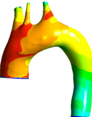
Figure 10: 3D modelling of aortic pressure wall of the healthy patient
A: from 2D PC MRI data, "controlled pressure" scenario
Figure 11: Comparison of 3D model of aortic wall shear stress of the healthy patient
A: 3D modeling of aortic wall shear stress of the healthy patient from 2D PC MRI data,
"controlled pressure" scenario
B: 3D modeling of aortic wall shear stress of the healthy patient from 0D model simulation,
Figure 12: Comparison of 3D model of aortic blood velocities fields of the healthy patient
A: 3D modeling of velocities fields in the aorta of the healthy patient from 2D CP MRI data,
"controlled pressure" scenario
B: 3D modeling of velocities fields in the aorta of the healthy patient from 0D model
Figure 13: 3D modelling of aortic pressure wall of the dissected patient
A: from 0D model simulation, "controlled pressure" scenario
B: from 2D CP MRI data, "moderately controlled pressure" scenario
Figure 14: 3D Modeling of aortic wall shear stress of the dissected patient
A: from 0D model simulation, "controlled pressure" scenario
B: from 2D CP MRI data, "moderately controlled pressure" scenario
C: from 0D model simulation, "high pressure by vasoconstriction" scenario
Figure 15: 3D modelling of aortic blood velocities field of the dissected patient
A: from 0D model simulation, "controlled pressure" scenario
B: from 2D CP MRI data, "moderately controlled pressure" scenario