HAL Id: hal-00301301
https://hal.archives-ouvertes.fr/hal-00301301
Submitted on 18 Jun 2004HAL is a multi-disciplinary open access
archive for the deposit and dissemination of sci-entific research documents, whether they are pub-lished or not. The documents may come from teaching and research institutions in France or abroad, or from public or private research centers.
L’archive ouverte pluridisciplinaire HAL, est destinée au dépôt et à la diffusion de documents scientifiques de niveau recherche, publiés ou non, émanant des établissements d’enseignement et de recherche français ou étrangers, des laboratoires publics ou privés.
Stratosphere-troposphere exchange from the Lagrangian
perspective: a case study and method sensitivities
M. S. Bourqui
To cite this version:
M. S. Bourqui. Stratosphere-troposphere exchange from the Lagrangian perspective: a case study and method sensitivities. Atmospheric Chemistry and Physics Discussions, European Geosciences Union, 2004, 4 (3), pp.3249-3284. �hal-00301301�
ACPD
4, 3249–3284, 2004 Stratosphere-troposphere exchange: a case study M. S. Bourqui Title Page Abstract Introduction Conclusions References Tables Figures J I J I Back CloseFull Screen / Esc
Print Version Interactive Discussion
© EGU 2004 Atmos. Chem. Phys. Discuss., 4, 3249–3284, 2004
www.atmos-chem-phys.org/acpd/4/3249/ SRef-ID: 1680-7375/acpd/2004-4-3249 © European Geosciences Union 2004
Atmospheric Chemistry and Physics Discussions
Stratosphere-troposphere exchange from
the Lagrangian perspective: a case study
and method sensitivities
M. S. Bourqui
Institute for Atmospheric and Climate Science, ETHZ, Switzerland
Received: 30 April 2004 – Accepted: 4 June 2004 – Published: 18 June 2004 Correspondence to: M. S. Bourqui ([email protected])
ACPD
4, 3249–3284, 2004 Stratosphere-troposphere exchange: a case study M. S. Bourqui Title Page Abstract Introduction Conclusions References Tables Figures J I J I Back CloseFull Screen / Esc
Print Version Interactive Discussion
© EGU 2004
Abstract
An important part of extra-tropical stratosphere-to-troposphere transport occurs in as-sociation with baroclinic wave breaking and cut-off decay at the tropopause. In the last decade many studies have attempted to estimate stratosphere-troposphere exchange (STE) in such synoptic events with various methods, and more recently efforts have 5
been put on inter-comparing these methods. However, large uncertainties remain on the sensitivities to methods intrinsic parameters, and on the best measure for STE with regard to end effects on chemistry.
The goal of the present study is to address these two fundamental issues in the con-text of the application of a trajectory-based Lagrangian method, which has been applied 10
in the past to climatological studies and has also been involved in inter-comparison studies, to a typical baroclinic wave breaking event.
The analysis sheds light on (i) the fine mesoscale temporal and spatial structures that are associated with episodic, rapid inflows of stratospheric air into the troposphere; (ii) the spatial resolution of 1◦×1◦ required to reasonably capture STE fluxes in such 15
a wave breaking event; (iii) the effective removal of spurious exchange events using a threshold residence time; (iv) the relevance of residence time distributions for capturing the effective chemical forcing of STE; (v) the large differences in the temporal evolution and geographical distribution of STE fluxes across the 2 and the 4 potential vorticity unit iso-surface definitions of the tropopause.
20
1. Introduction
The exchange of mass between the stratosphere and the troposphere has important implications for climate and life conditions on the earth’s surface. Injection of ozone-rich stratospheric air into the troposphere is recognised to significantly force the chem-istry and subsequently the radiation (e.g.Roelofs and Lelieveld, 1997), and can en-25
ACPD
4, 3249–3284, 2004 Stratosphere-troposphere exchange: a case study M. S. Bourqui Title Page Abstract Introduction Conclusions References Tables Figures J I J I Back CloseFull Screen / Esc
Print Version Interactive Discussion
© EGU 2004 2002). Transport of tropospheric air (with natural and anthropogenic emissions) into
the stratosphere perturbs the stratospheric chemistry and can have consequences as important as stratospheric ozone depletion. For convenience, we use hereafter the abbreviations STT for stratosphere-to-troposphere transport, TST for troposphere-to-stratosphere transport, and STE for general troposphere-to-stratosphere-troposphere exchange. 5
STE has received a lot of attention during the last two decades, and some key prop-erties have been identified.
On the one hand, STE can be seen to some extent as the lowest branch of the Brewer-Dobson circulation (Holton et al., 1995). The latter, understood here as the mean residual circulation resulting from the Transformed Eulerian Mean framework 10
(Andrews et al.,1987), is mainly driven by planetary wave breaking within the middle stratosphere ’surf zone’ (McIntyre and Palmer, 1983; Haynes et al., 1991). Yet, the vertical mass flux in the tropopause region associated with this circulation exhibits very different distributions whether it is calculated across PV1 iso-surfaces, isentropes or isobaric surfaces, due to the different vertical motion of these surfaces relative to the 15
flow (Juckes, 2001). On the other hand, tropospheric dynamics influence to a large extent the tropopause region and hence the flux across the tropopause.
In the extra-tropics, injection of stratospheric air into the troposphere has been detected almost exclusively in regions of upper-level troughs and cut-off lows (e.g. Danielsen, 1980; Shapiro, 1980; Ancellet et al., 1991; Langford et al., 1996; Eisele 20
et al.,1999). These structures are part of baroclinic wave life-cycles and are frequently associated with the production of folding and filamentation structures (e.g.Bush and Peltier, 1994;Bithell et al.,1999). The physical processes responsible for STT have been analysed in numerous studies and a variety of mechanisms has been identi-fied. Their relative importance varies significantly from case to case. The presence of 25
clouds in the upper-troposphere (often induced on the warm, downstream side of an upper-level trough) and the associated latent heat release leads systematically to a sig-nificant inflow of stratospheric air into the troposphere (e.g.Lamarque and Hess,1994;
1
ACPD
4, 3249–3284, 2004 Stratosphere-troposphere exchange: a case study M. S. Bourqui Title Page Abstract Introduction Conclusions References Tables Figures J I J I Back CloseFull Screen / Esc
Print Version Interactive Discussion
© EGU 2004 Wirth,1995a). Turbulence in the region of the jet stream in absence of clouds (clear air
turbulence) has been identified (Shapiro,1976) and its significance for stratosphere-troposphere exchange demonstrated (Shapiro, 1980). The formation of small-scale filaments or folds and their irreversible mixing is also recognised to account for a signif-icant part of the overall exchanged mass (e.g.Price and Vaughan,1993;Hartjenstein, 5
2000). A few studies have also analysed the physical processes involved in TST in the extra-tropics. Radiative effects in anticyclones, in particular those related to the water vapour profile, can induce upward transport (e.g.Hoskins et al.,1985;Zierl and Wirth, 1997). Additionally, intense convective complexes which overshoot the tropopause are likely to inject tropospheric air into the stratosphere at the anvil outflow (e.g. Poulida 10
et al.,1996;Stenchikov et al.,1996) or via breaking of gravity waves generated above cumulus clouds (Wang,2003).
Methods estimating STE at synoptic scales must be able to resolve the motions of the flow and of the tropopause at the scales on which the involved physical processes are acting, otherwise they may misrepresent the differential motion of the flow and the 15
tropopause. However, if such methods are to produce estimates on the global scale, they must in addition be applicable to global meteorological data with synoptic-scale resolution such as operational (re-)analysis data. In past studies, such quantifications have been carried out using merely four types of methods: (1) the methods based upon Eulerian formulations of the cross-tropopause flux and estimating individual terms of 20
the formulation (e.g.Wei,1987;Wirth,1995b;Wirth and Egger,1999), (2) the methods explicitely estimating the non-advective part of the motion of the tropopause (Lamarque and Hess,1994;Wirth and Egger,1999), (3) the methods using a trajectory-based La-grangian representation of the flow (e.g.Wernli and Davies,1997;Stohl,2001;Wernli and Bourqui,2002), (4) the methods using transport schemes with physics parameter-25
izations and estimating the cross-tropopause transport of a passive tracer (e.g.Gray, 2003).
The study ofWirth and Egger(1999) inter-compared in the context of a case-study several methods based on Eulerian formulations and a method of type (2) employing
ACPD
4, 3249–3284, 2004 Stratosphere-troposphere exchange: a case study M. S. Bourqui Title Page Abstract Introduction Conclusions References Tables Figures J I J I Back CloseFull Screen / Esc
Print Version Interactive Discussion
© EGU 2004 trajectories. They suggested that methods of type (1) produce reasonable estimates
when formulated with a PV-vertical coordinate and produce noisy estimates in all other cases. Note that the PV-vertical coordinate formulation of the mass flux requires a direct estimate of the material derivative of PV. This quantity was available as model output in the study ofWirth and Egger(1999), but can not in general be derived from 5
meteorological fields with a reasonable confidence. They also suggested that type (2) methods produce reliable estimates. In another inter-comparison study,Kowol-Santen et al. (2000) estimated STE from a mesoscale model output with a type (1) methodol-ogy formulated in isentropic vertical coordinates and a type (3) method. Although the net mass flux estimated from the two methods was in agreement, the separated STT 10
and TST mass fluxes were found noisier in the type (1) method.
Wernli and Bourqui(2002) recently introduced a Lagrangian method using a “thresh-old residence time”. This method is based on a representation of the flow by three-dimensional trajectories, started from a dense three-three-dimensional grid and computed using wind fields from the European Centre for Medium-Range Weather Forecasts 15
(ECMWF) operational analyses. Exchange events are then selected from the trajec-tories that reside within the troposphere and the stratosphere before and after having crossed the tropopause for a period longer than a given threshold residence time τ∗. They produced a one-year climatology of exchange in the extra-tropical northern hemi-sphere with a detailed geographical distribution which was in quantitative agreement 20
with independent results from methods cast in the zonal mean framework. The exten-sion of the climatology to fifteen years merely confirmed these results (Sprenger and Wernli,2003).
Within the recent EU project STACCATO (Stohl et al.,2003), this trajectory-based Lagrangian method took part in a method inter-comparison and verification exercise 25
based upon selected case studies of STE in the European sector (Meloen et al.,2003; Cristofanelli et al.,2003). The inter-comparison included in particular Lagrangian trans-port models with physics parameterizations, chemical transtrans-port models and general circulation models (type 4). It was shown that purely trajectory-based approaches
ACPD
4, 3249–3284, 2004 Stratosphere-troposphere exchange: a case study M. S. Bourqui Title Page Abstract Introduction Conclusions References Tables Figures J I J I Back CloseFull Screen / Esc
Print Version Interactive Discussion
© EGU 2004 yield lower bound estimates of STE because they capture the large-scale transport but
no turbulent nor diffusive processes. Particle dispersion models with parameterized turbulence led to slightly larger cross-tropopause mass fluxes, while estimates from relatively coarse scale global models were distinctively larger and were shown to suf-fer from numerical diffusion. Indeed, for the cases under consideration, based upon a 5
limited observational data set available for validation, and in sight of the uncertainties implied by parameterizations on transport, the trajectory-based Lagrangian approach accurately identified regions subject to stratosphere-to-troposphere transport and pro-vided quantitative estimates that can be regarded as realistic lower bounds.
The independent study of Gray(2003) suggested also, using a passive tracer in a 10
mesoscale model, that a large part of the cross-tropopause mass flux comes from the model explicit advection, with still a maximum of 38% attributed to parameterized convection and to a lesser extend to parameterized turbulent mixing. They showed in addition a substantial sensitivity of the estimates to the horizontal resolution.
A key element introduced in the study ofWernli and Bourqui(2002) was the thresh-15
old residence time, used to select the “significant” exchange events. They suggested that anticipated errors in the mass flux due to derivation of PV and trajectory calcu-lation were likely to introduce spurious exchange events mostly associated with small residence times. Based upon this assumption and the fact that small residence times imply potentially weak chemical action, they suggested to filter out the small residence 20
time events by employing a threshold residence time. Interestingly, the dependence of their mass flux estimates STT and TST with the threshold residence time did not seem to converge to any fixed flux within the range of residence times of days. A recent theoretical work has been carried out on this question byHall and Holzer(2003). They concluded that in the small threshold residence time limit, in absence of scale limi-25
tations, the separated fluxes diverge, or equivalently, the gross fluxes are completely dominated by fluid elements residing infinitesimally. And in presence of scale limita-tions due to finite data resolution, the gross fluxes are dominated by the smallest scales resolved.
ACPD
4, 3249–3284, 2004 Stratosphere-troposphere exchange: a case study M. S. Bourqui Title Page Abstract Introduction Conclusions References Tables Figures J I J I Back CloseFull Screen / Esc
Print Version Interactive Discussion
© EGU 2004 The motivation of the present study is to gain a deeper understanding of the
method-ology introduced in Wernli and Bourqui (2002), and along with this a deeper un-derstanding of basic cross-tropopause transport properties, in the context of a case study with special emphases on the residence time, the data resolution and the PV-tropopause definition. In addition, the potential offered by the method for detailed 5
physical analyses of the processes involved is illustrated.
The structure of the paper is as follows. In Sect. 2 we describe the data set and the Lagrangian method. Then, in Sect. 3 the baroclinic wave event under consideration is rapidly described, results of STE estimates are presented and further details are shown using three-dimensional views. In Sect. 4 is discussed the sensitivity of the method to 10
data resolution, threshold residence time and the PV-tropopause definition. And finally, conclusions are drawn in Sect. 5.
2. Data and method
The cross-tropopause flux calculation is based on hourly outputs of the limited-area Europa Model (EM) of the German Weather Service (Majewski,1991). The resolution 15
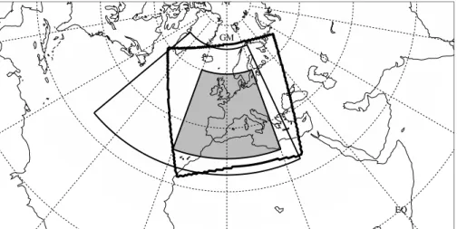
in the model is 0.5◦×0.5◦in the horizontal and 40 levels in the vertical2. The hindcast simulation is performed for a duration of 162 h from 1 September 1997, 00:00 UTC to 7 September 1997, 18:00 UTC, and uses the six-hourly ECMWF analysis fields (T213L31) as initial and boundary conditions. The simulation domain is drawn in Fig.1 by the bold line. The simulation results compare reasonably well with the ver-20
ifying ECMWF analyses (not shown), and reproduce correctly the different phases of the synoptic and mesoscale development both in amplitude and location. A slightly smaller domain than the simulation domain is used for the quantification of exchange (see Fig.1, filled domain). To enable the computation of trajectories outside the
simu-2
Levels every 20 hPa in the tropopause region between 150 and 510 hPa, and every 30 hPa elsewhere with the top level at 30 hPa.
ACPD
4, 3249–3284, 2004 Stratosphere-troposphere exchange: a case study M. S. Bourqui Title Page Abstract Introduction Conclusions References Tables Figures J I J I Back CloseFull Screen / Esc
Print Version Interactive Discussion
© EGU 2004 lation domain ECMWF analysis data are used to extend the data domain to the whole
northern hemisphere.
The method for quantifying the stratosphere-troposphere exchange flux is an adap-tation of the trajectory-based method introduced byWernli and Bourqui(2002) allowing for a higher temporal and spatial resolution of the data within a limited area (Bourqui, 5
2001). We summarise here the main features of the method and the parameters that were used to achieve the results presented in Sect. 3. The sensitivity of the method to the main parameters is discussed in Sect. 4.
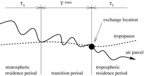
The definition of an exchange event is based on the condition that the trajectory re-sides for a time period longer than a given threshold residence time τ∗in either sides of 10
the tropopause before and after having crossed the tropopause (see schematic illustra-tion in Fig.2). The trajectories are computed with the three-dimensional LAGRangian ANalysis TOol LAGRANTO (Wernli and Davies,1997) based on Petterssen’s kinematic method (Petterssen,1956). In this study, the 2 PVU3iso-surface is used as tropopause definition because it mimics reasonably well the thermal tropopause in the extra-tropics 15
(Holton et al.,1995) and is a well-defined, continuous surface with conservation prop-erties.
The set of exchange trajectories is obtained by a three-step computation scheme. First, the time-dependent flow is discretisized spatially and temporally into a set of tra-jectories. The trajectories are started every 12 h for a length of 12 h from a starting grid 20
extending vertically from 600 to 50 hPa and horizontally as shown in Fig.1. The starting points are separated from each other horizontally by 0.5◦ and vertically by 5 hPa, so that each trajectory represents an air mass∆m= g−1·∆x·∆y·∆p≈157×109kg. Second, the 12 h trajectories which cross the 2 PVU iso-surface are prolongated for 5 days both backwards and forwards. Third, the selection is performed on every prolongated trajec-25
tory according to the conceptual model illustrated in Fig.2. Each trajectory must reside within the troposphere and the stratosphere for time periods longer than the threshold residence time τ∗. The two residence time periods, within the troposphere and within
3
ACPD
4, 3249–3284, 2004 Stratosphere-troposphere exchange: a case study M. S. Bourqui Title Page Abstract Introduction Conclusions References Tables Figures J I J I Back CloseFull Screen / Esc
Print Version Interactive Discussion
© EGU 2004 the stratosphere, are separated by a transition time smaller than Tmaxtrans. This maximum
transition time allows the trajectories to oscillate around the tropopause while crossing it. The parameters used here are 12 h for the threshold residence time τ∗ and 6 h for the maximum transition time Tmaxtrans.
Finally, the exchange mass flux is given by the sum of the mass transported by 5
the trajectories which experience an exchange within a 1◦×1◦grid-square during each period of 12 h.
In essence, this method is identical to the one used byWernli and Bourqui(2002). The transition period of 6 h is introduced here only because of the increased temporal data resolution.
10
3. Results
3.1. Synoptic evolution of the tropopause
The synoptic situation corresponds to the late stage of a typical baroclinic wave de-velopment similar to the anticyclonic-shear case described by Davies et al. (1991) and Thorncroft et al. (1993), and includes the break-up of a stratospheric streamer4 15
and the decay of the resulting cut-off. Figure 3 shows the time sequence of poten-tial temperature interpolated onto the 2 PVU iso-surface and the presence of clouds at 350 hPa (red contours). The two-dimensional representation of the tropopause pro-vided in Fig.3gives some indication of its vertical structure, however without showing folded structures (in case of folded structures, only the highest level is represented). 20
The dynamical interpretation of these maps is similar to that of isentropic potential vorticity charts (Hoskins et al.,1985;Hoskins,1991).
The elongated, north-south oriented streamer arrives over western Europe and
be-4
FollowingAppenzeller et al.(1996), a streamer is a synoptic-scale equatorward advection of high potential vorticity on an isentropic PV map.
ACPD
4, 3249–3284, 2004 Stratosphere-troposphere exchange: a case study M. S. Bourqui Title Page Abstract Introduction Conclusions References Tables Figures J I J I Back CloseFull Screen / Esc
Print Version Interactive Discussion
© EGU 2004 gins to break on 1 September around 12:00 UTC. It takes about 3 days to break up all
isentropic contours in the range 325–340 K on the 2 PVU tropopause. However, most of the tropopause irreversible deformation associated with the break-up occurs between 1 Septtember, 06:00 UTC and 2 September, 06:00 UTC (Fig.3a–c). During this period, a cloud forms and decays right on the eastern edge of the streamer. It is followed to the 5
east by another cloud formation which disappears on 3 September, 06:00 UTC. These cumulus cloud formations are triggered by the northward and upward advection of hu-mid air driven by the cyclonic circulation induced by the streamer itself, and are proba-bly reinforced by the passage of moist air over the Pyrenees. Then, from 2 September, 06:00 UTC, the resulting PV cut-off, located over the Mediterranean, is clearly detached 10
from the parent wave structure from 3 September, 06:00 UTC onwards (Fig.3e–h). It starts immediately to decay and almost disappears by 5 September, 00:00 UTC. 3.2. Estimates of stratosphere-troposphere exchange
Figure 4 gives the sequence of the 12-h integrated net mass exchange between 1 September, 00:00 UTC and 5 September, 00:00 UTC. On the time scale of 12 h TST 15
and STT occur principally in geographically separated regions, and therefore the net flux gives a fairly comprehensive representation of the separated fluxes: positive for STT and negative for TST.
The general structure of STE patterns reveals well identifiable zones of strong ex-change activity and a relatively weak background. The active zones are confined in 20
space and time and occur almost exclusively in the region of the stratospheric intru-sion. Two major exchange episodes can be identified:
(1) On 1 Septtember, 12:00–24:00 UTC (Fig.4b) a distinct structure of strong STT is found in association with the breaking of the streamer. Exchange is concentrated at the streamer’s tip and in the zone of irreversible deformation where the break-up 25
occurs and a cut-off detaches from the polar PV reservoir.
ACPD
4, 3249–3284, 2004 Stratosphere-troposphere exchange: a case study M. S. Bourqui Title Page Abstract Introduction Conclusions References Tables Figures J I J I Back CloseFull Screen / Esc
Print Version Interactive Discussion
© EGU 2004 occurs around the cut-off low and then towards its centre. This exchange pattern
is related to the slow decay of the cut-off.
Some weaker but still distinct structures can also be seen. For instance, on 2 Septem-ber, 00:00–12:00 UTC (Fig.4c) east of the streamer a region of exchange is observed in association with the locally raised tropopause above the cloud (Fig.3c). And on 3 5
September, 12:00–24:00 UTC (Fig.4f), a north-south oriented tongue of TST is located to the west of the stretching zone, and is related to the thin “tropospheric streamer5” which occurs in this region (Fig.3f).
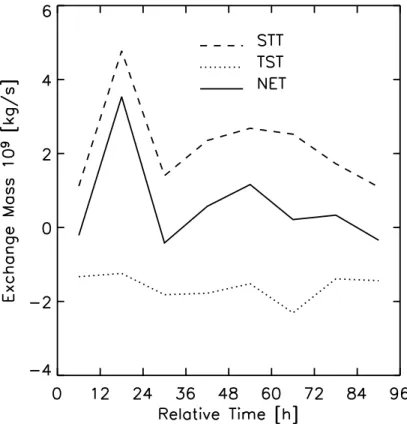
The time evolution of total mass exchange associated with the synoptic development is provided in Fig. 5. The two major STE events are clearly visible. The total STT 10
associated with the streamer break-up episode is 206×1012kg (1 September, 12:00– 24:00 UTC), and with the cut-off decay episode 288×1012kg (3 September, 12:00– 24:00 UTC). These two episodes led to a comparable mass exchange although the rate of exchange was roughly four times larger in the first one. The TST time evolution does not show any major exchange episode, so that the net transport follows roughly 15
the STT time evolution.
For the entire four days period, the overall mass exchange amounts to 763×1012kg for STT, 554×1012kg for TST, and 209×1012kg for the net transport.
3.3. Details of the streamer break-up episode
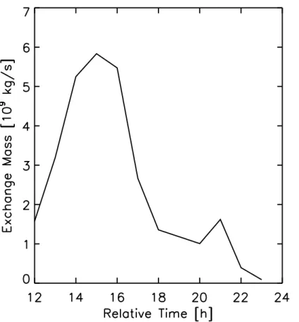
The detailed hourly development of the net mass flux during the streamer break-up 20
episode is represented in Fig. 6 between 12:00 and 24:00 UTC of 1 September. It reveals that the exchange of mass attributed to the streamer break-up is limited to a time period of only 6 h, with a peak at 15:00–16:00 UTC.
5
A tropospheric streamer denotes the reverse of a stratospheric streamer, i.e. an elongated pool of tropospheric air with low PV values stretching northwards which can be seen on an isentropic PV map.
ACPD
4, 3249–3284, 2004 Stratosphere-troposphere exchange: a case study M. S. Bourqui Title Page Abstract Introduction Conclusions References Tables Figures J I J I Back CloseFull Screen / Esc
Print Version Interactive Discussion
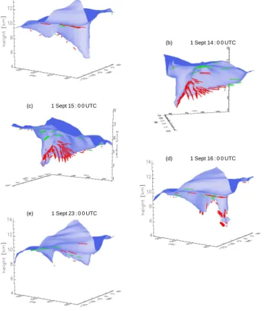
© EGU 2004 Five stages of the three-dimensional tropopause evolution during this explosive
break-up are presented in Fig. 7: (a) well before (10:00 UTC), (b) near the begin-ning (14:00 UTC), (c) at the maximum (15:00 UTC), (d) near the end (16:00 UTC), and (e) well after (23:00 UTC) the event. At 10:00 UTC (Fig.7a), the tropopause penetrates deeply into the troposphere and reaches elevations down to 5–6 km. The intrusion has 5
a smooth vertical flank which rolls up cyclonically at the southern tip. The bottom of the flank is nearly aligned with isentropic surfaces. Then, between 14:00 UTC and 16:00 UTC, the flank is rapidly eroded. An arched structure is progressively formed, leading to a “child” intrusion at the northern boundary and an isolated vertical tube at the southern boundary (Fig.7d). And finally (Fig.7e), the lower part of the stratospheric 10
tube is entirely mixed and the tropopause resembles its state eleven hours earlier but with a much shallower intrusion.
The temporal evolution of the tropopause erosion shown in Fig.7gives credit to our estimates of the hourly evolution of exchange mass flux shown in Fig.6. In particular, the mass flux peaks at 15:00 UTC while the tropopause is experiencing its strongest 15
irreversible deformation. STT and TST trajectories are represented near the exchange time as red and green traces in Fig.6. There is an excellent agreement between the diagnosed locations of STT events and the zone of erosion of the tropopause.
This detailed time sequence also reveals how a large amount of stratospheric air mass can be injected into the troposphere on the mesoscale.
20
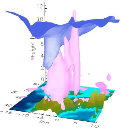
The streamer break-up coincides temporally with the intense cumulus cell east of the streamer and north of the Pyrenees. The cloud cell strengthens and grows vertically as the streamer is advected eastwards. It reaches a maximum size between 14:00 and 17:00 UTC and then decays very rapidly. Figure8represents the cloud cell relatively to the tropopause at 14:00 UTC. Comparison of (i) the time evolution of this cloud with that 25
of exchange and (ii) the position and shape of the cloud with the locations of exchange in Figs.7 and 8, gives first indications that exchange is triggered by the cloud. Note that in this case most exchange events take place on the side of the cloud, and nearly no events are found directly above the cloud (Fig.4b). However, a detailed analysis of
ACPD
4, 3249–3284, 2004 Stratosphere-troposphere exchange: a case study M. S. Bourqui Title Page Abstract Introduction Conclusions References Tables Figures J I J I Back CloseFull Screen / Esc
Print Version Interactive Discussion
© EGU 2004 the exchange processes is beyond the scope of this paper.
4. Sensitivity analyses
4.1. Sensitivity to data resolution
The STE flux estimates described in the previous section have been repeated for vari-ous data resolutions obtained by degradation of the original data set (0.5◦× 0.5◦×1 h). 5
All trajectories as well as the tropopause have been re-computed using the coarser, degraded data. This method allows to keep exactly the same meteorological evolution at every resolution. The temporal evolution of total cross-tropopause mass flux for the various data resolutions is shown in Fig.9separately when degrading space and time resolutions.
10
The STT results show a clear response to varying spatial resolutions. While the 0.5◦ and 1◦ resolutions lead roughly to similar results, the 2◦ resolution produces a strong underestimate of STT during the break-up phase as well as the late cut-off de-cay phase. This underestimate is obviously due to a too coarse representation of the tropopause deformation. A slight underestimate of STT in the late cut-off decay phase 15
is also seen with the 1◦ resolution, which indicates that structures of a scale smaller than 1◦ contribute to the cut-off decay, though to a small extent. TST estimates do not show a clear response to the degradation of spatial resolution. The 1◦ resolution pro-duces substantially larger values, while the 2◦resolution gets a very different temporal structure. This unexpected response is thought to be caused by the simple data degra-20
dation scheme which produces an anomalously large variability in the vertical velocity of low resolution fields, in particular in the tropopshere. The resulting net flux shows a reduced magnitude at low spatial resolutions, but keeps its gross temporal structure. The total net mass flux over the whole period of 96 h is very sensitive to the horizontal resolution: 209×1012kg at 0.5◦resolution, 27×1012kg at 1◦, and −15×1012kg at 2◦. 25
ACPD
4, 3249–3284, 2004 Stratosphere-troposphere exchange: a case study M. S. Bourqui Title Page Abstract Introduction Conclusions References Tables Figures J I J I Back CloseFull Screen / Esc
Print Version Interactive Discussion
© EGU 2004 resolution, the STT is slightly overestimated during the late cut-off decay phase at the
3 h resolution, while it is increased by a quasi-constant noise at the 6 h resolution. The TST responds in a similar way. The noise introduced in both STT and TST mostly cancels in the net mass flux, and thanks to this symmetry, the effect of the temporal resolution on the total net mass flux becomes relatively smaller: 209×1012kg at 1 h 5
resolution, 138×1012kg at 3 h resolution, and 128×1012kg at 6 h resolution. Note that the latter considerations also hold for a spatial resolution of 1◦instead of the 0.5◦ (not shown).
4.2. Sensitivity to threshold residence time
The spatial smoothening of the tropopause, consequence of the derivation of PV from 10
limited resolution data, and the interpolations within the trajectory calculation scheme are suspected to produce oscillations of trajectories around the tropopause even if the flow is PV-conservative. This may introduce lots of spurious exchange events with rather short residence times. Some information on these spurious events can be gained by hypothesizing that lowering the spatial resolution increases the smoothening 15
of the tropopause, and hence increases the number of spurious exchange events. An extra experiment has been carried out to investigate specifically this question. For every data resolutions, 90 h long trajectories have been started from our usual starting grid forward in time on 1 September, 00:00 UTC and backwards on 4 Septem-ber, 18:00 UTC. The distributions of time intervals between two successive cross-20
tropopause events along the trajectories, both happening within the simulation domain, are shown in Fig.10. Obviously, the general shape of the distributions are strongly constrained by the length of trajectories and the requirement that successive crossing points must be within the simulation domain. To account for this constraint and other possible effects of the system, we use the 0.5◦, 1 h resolution distribution as reference 25
distribution. Compared to this reference distribution, the distributions for lower spatial resolutions with 1 h temporal resolution show remarkable increased frequencies of in-terval times smaller than about 8 h, and no significant difference above. The effects of
ACPD
4, 3249–3284, 2004 Stratosphere-troposphere exchange: a case study M. S. Bourqui Title Page Abstract Introduction Conclusions References Tables Figures J I J I Back CloseFull Screen / Esc
Print Version Interactive Discussion
© EGU 2004 lower temporal resolutions is a truncation of the distribution of interval times lower than
about the temporal resolution itself.
This result justifies the hypothesis that lowered spatial resolutions induce more spu-rious cross-tropopause events. And furthermore, it shows clearly that spuspu-rious events can be removed to a large extent by setting a threshold residence time larger than 8 h. 5
The dependence with the threshold residence time of the temporal evolution of STE for the highest data resolution is shown in Fig. 11. A confirmation of the ability of the residence time criterion to remove properly spurious events comes from the com-parison of STE estimates with τ∗=12 h and without residence time criterion. In effect, although the raw STE fluxes are three to five times larger than the STE fluxes with 10
τ∗=12 h, and although the temporal evolution differ strongly, the net fluxes are very
similar. This demonstrates that a large number of exchange events in the raw STE fluxes are associated with residence time smaller than 12 h which cancel each other in the net flux at each time step. The cross-tropopause flux estimated with the residence time criterion preserves the relevant exchange fluxes, and leads to a net flux which is 15
of the same order of magnitude as the individual STT and TST.
For τ∗≥12 h, the dependence of the STE fluxes with τ∗ is smaller and is more or less constant throughout the temporal evolution. Slightly different dependences on τ∗ can nevertheless be seen, as for instance in the begining of the cut-off decay, where fewer short residence times than normal are present in the STT. This illustrates how 20
a broader layer around the tropopause can influence the cross-tropopause mass flux when estimated as a function of τ∗.
Note finally that the problem of inability in estimating the exchange flux at residence times lower than about 8 h is not specific of the Lagrangian approach, but also per-tains, in a dissimulated way, to the Eulerian approach. In effect, the Eulerian approach 25
couples time derivatives with spatial derivatives of limited resolution data and this way introduces spurious exchange fluxes.
ACPD
4, 3249–3284, 2004 Stratosphere-troposphere exchange: a case study M. S. Bourqui Title Page Abstract Introduction Conclusions References Tables Figures J I J I Back CloseFull Screen / Esc
Print Version Interactive Discussion
© EGU 2004 4.3. Dependence on the PV-tropopause definition
The STE mass flux can significantly differ depending on the applied tropopause defi-nition. Here, we explore the dependence of STT and TST on the PV-level defining the dynamical tropopause over a range between 1.5 and 5 PVU.
Figure12 shows the temporal evolution of STT, TST and NET mass fluxes. In gen-5
eral, for both STT and TST, the mass flux is monotonically decreasing with the PV level, but the function of the PV level is not constant along the time and clearly depends on the synoptics. In particular, the STT associated with the explosive streamer break-up and with the cut-off decay occurs only at levels below 4 PVU. Above 4 PVU, a differ-ent, flater temporal evolution is seen, with largest STT taking place during the period 10
1 September, 12:00 UTC–3 September, 00:00 UTC. The NET mass flux shows also a strong contrast between the levels below 4 PVU, where the break-up and cut-off de-cay phases are captured, and the levels above, again dominated by the 1 September, 12:00 UTC–3 September, 00:00 UTC period.
The synoptics of exchange patterns for the different PV levels during the explosive 15
break-up phase is shown in Fig. 13. In the streamer’s tip, STT occurs exclusively at levels below 4 PVU, while in the region where isentropic PV contours break from the polar high PV reservoir, STT is seen over the whole range of PV levels. Note that these graphs have been scaled individually to put emphasis on the spatial structure. As the overall magnitude of STT decreases with higher PV levels, TST becomes relatively 20
more important. At 5 PVU the magnitudes are comparable and the dominating patterns of both STT and TST are compact and tied to the streamer, with TST on the western edge of the streamer and in the Y structure to the north, and STT within the streamer.
An important consequence is that the 4 PVU iso-surface can not be considered as a proxy of PV levels underneath as far as STE is concerned.
ACPD
4, 3249–3284, 2004 Stratosphere-troposphere exchange: a case study M. S. Bourqui Title Page Abstract Introduction Conclusions References Tables Figures J I J I Back CloseFull Screen / Esc
Print Version Interactive Discussion
© EGU 2004
5. Conclusions
In this study, STE mass flux was estimated within a typical baroclinic wave breaking event and subsequent cut-off decay using a method adapted fromWernli and Bourqui (2002). The detailed analysis of STE associated with the event illustrated how fine temporal and spatial mechanisms can lead to large mass fluxes across the tropopause. 5
In particular we showed the explosive nature of the streamer breakup, which happened over a period of 4–6 h. The two phases of the synoptic evolution that are the break-up and the cut-off decay were found to contribute to a similar extent in the total exchange mass flux.
A comparison of our results with other published estimates is shown in Table1. Our 10
estimates are of comparable magnitude, though rather on the lower edge of the range of estimates of these other studies. A reason for having relatively small values may come from the threshold residence time, which filters out the part of the mass flux associated with τ∗<12 h. However, it must be emphasized that the variety of synoptic
situations, seasons, and the sizes of domains and time windows over which mass 15
fluxes are averaged are all factors which, beside the remaining uncertainties in the methodologies, contribute to enlarge the range of estimates.
Furthermore, the comparison of the total mass flux obtained in this case study with the autumn mass flux in the European sector ofWernli and Bourqui(2002) suggests that tropopause perturbations like the one studied here may just follow one another 20
every 3-5 days on average, and this way, produce frequent, episodical transport of mass across the tropopause.
The analysis of the sensitivity of the method to key parameters led to the following conclusions:
Data resolution: The sensitivity to the spatial resolution arises mostly from the scale
25
required to correctly represent the processes that play relevant roles. A data resolution of 1◦×1◦is found to give correct estimates of STT, and a resolution of 2◦×2◦ is found to be too coarse. The large sensitivity of TST to spatial resolution is thought to be mainly
ACPD
4, 3249–3284, 2004 Stratosphere-troposphere exchange: a case study M. S. Bourqui Title Page Abstract Introduction Conclusions References Tables Figures J I J I Back CloseFull Screen / Esc
Print Version Interactive Discussion
© EGU 2004 caused by an artefact in the degradation method and needs to be further studied. The
sensitivity to temporal resolution showed that a nearly constant noise was introduced at the 6 h resolution in both STT and TST, which mostly cancels in the net flux.
Threshold residence time: The threshold residence time is found to be very effective
in removing spurious exchange events, as spurious events are largely associated with 5
residence times smaller than 8 h. It is also shown that STT and TST fluxes are associ-ated with continuous distributions of residence times which can vary depending on the synoptics. As a consequence, there is no unique choice for the threshold residence time, and larger values of τ∗can be used to emphasize more significant exchanges.
PV-level tropopause: STE estimates showed also an interesting dependence on the
10
choice of the PV-level defining the tropopause. The mass transported across PV-levels higher than or equal to 4 PVU showed a different global evolution, with the largest part of STT occuring at the break-up of the streamer, no STT at the streamer’s tip and weak STT around the cut-off during its decay phase.
The chemistry of the troposphere and the lower stratosphere is very sensitive to 15
cross-tropopause inflows, and a few important consequences for the chemistry can be drawn from this study:
(i) The use of rough STE fluxes without removing spurious exchanges would lead to a dramatic overestimate of the chemical effect of STE.
(ii) The effective chemical action of exchanged masses is closely related to the resi-20
dence time distribution associated with exchange. In particular, both the flux across the tropopause and the transport properties in the upper-troposphere and lower-stratosphere are key for estimating/modelling chemical effects of STE.
(iii) The mass flux across iso-PV surfaces has different patterns above and below 4 PVU, which suggests that STE estimated across the 4 PVU or 5 PVU iso-surfaces 25
can not be used as a proxy for the 2 PVU. Furthermore, if we assume that the 2 PVU iso-surface acts as an upper boundary for the troposphere, inflow of stratospheric air into the troposphere must be considered across the 2 PVU surface. On the other hand, the inflow of tropospheric air into the stratosphere, as estimated across the 4 PVU
iso-ACPD
4, 3249–3284, 2004 Stratosphere-troposphere exchange: a case study M. S. Bourqui Title Page Abstract Introduction Conclusions References Tables Figures J I J I Back CloseFull Screen / Esc
Print Version Interactive Discussion
© EGU 2004 surface, may better represent the relevant patterns.
Acknowledgements. The author wishes to thank H. Wernli and H. Davies for many discussions
and valuable comments on earlier versions of this paper. Meteoswiss is thanked for providing access to ECMWF data.
References
5
Ancellet, G., Pelon, J., Beekmann, M., Papayannis, A., and M ´egie, G.: Ground-based studies of ozone exchanges between the stratosphere and the troposphere, J. Geophys. Res., 96, 22 401–22 421, 1991. 3251
Andrews, D. G., Holton, J. R., and Leovy, C. B.: Middle Atmosphere Dynamics, Academic Press, San Diego, Calif., 1987. 3251
10
Appenzeller, C., Davies, H. C., and Norton, W. A.: Fragmentation of stratospheric intrusions, J. Geophys. Res., 101, 1435–1456, 1996. 3257
Bithell, M., Gray, L. J., and Cox, B. D.: A three-dimensional view of the evolution of midlatitude stratospheric intrusions, J. Atmos. Sci., 56, 673–688, 1999. 3251
Bourqui, M.: Analysis and Quantification of STE: A Novel Approach, Ph.D. thesis, Swiss
Fed-15
eral Institute of Technology (ETH), 2001. 3256
Bush, A. B. G. and Peltier, W. R.: Tropopause folds and synoptic-scale baroclinic wave life cycles, J. Atmos. Sci., 51, 1581–1604, 1994. 3251
Cristofanelli, P., Bonasoni, P., Collins, W., Feichter, J., Forster, C., James, P., Kentarchos, A., Kubik, P. W., Land, C., Meloen, J., Roelofs, G. J., Siegmund, P., Sprenger, M., Schnabel, C.,
20
Stohl, A., Tobler, L., Tositti, L., Trickl, T., and Zanis, P.: Stratosphere-to-troposphere transport: A model and method evaluation, J. Geophys. Res., 108, 8525, doi:10.1029/2002JD002 600, 2003. 3253
Danielsen, E. F.: Stratospheric source for unexpectedly large values of ozone measured over the pacific ocean during Gametag, August 1977, J. Geophys. Res., 85, 401–412, 1980.
25
3251
Davies, H. C., Sch ¨ar, C., and Wernli, H.: The palette of fronts and cyclones within a baroclinic wave development, J. Atmos. Sci., 48, 1666–1689, 1991. 3257
Eisele, H., Scheel, H. E., Sladkovic, R., and Trickl, T.: High-resolution Lidar measurements of stratosphere-troposphere exchange, J. Atmos. Sci., 56, 319–330, 1999. 3251
ACPD
4, 3249–3284, 2004 Stratosphere-troposphere exchange: a case study M. S. Bourqui Title Page Abstract Introduction Conclusions References Tables Figures J I J I Back CloseFull Screen / Esc
Print Version Interactive Discussion
© EGU 2004
Gray, S. L.: A case study of stratosphere to troposphere transport: The role of con-vective transport and the sensitivity to model resolution, J. Geophys. Res., 108, 4590, doi:10.1029/2002JD003 317, 2003. 3252,3254,3271
Hall, T. M. and Holzer, M.: Advective-diffusive mass flux and implications for
stratosphere-5
tropopshere exchange, Geophys. Res. Lett., 30, 1222, doi:10.1029/2002GL016 419, 2003. 3254
Hartjenstein, G.: Diffusive decay of tropopause folds and the related cross-tropopause mass flux, Mon. Weather Rev., 128, 2958–2966, 2000. 3252
Haynes, P. H., Marks, C. J., McIntyre, M. E., Shepherd, T. G., and Shine, K. P.: On the
“down-10
ward control” of extratropical diabatic circulations by eddy-induced mean zonal forces, J. Atmos. Sci., 48, 651–678, 1991. 3251
Holton, J. R., Haynes, P. H., McIntyre, M. E., Douglass, A. R., Rood, R. B., and Pfister, L.: Stratosphere-troposphere exchange, Rev. Geophys., 33, 403–439, 1995. 3251,3256 Hoskins, B. J.: Towards a PV-θ view of the general circulation, Tellus, 43, 27–35, 1991. 3257
15
Hoskins, B. J., McIntyre, M. E., and Robertson, A. W.: On the use and significance of isentropic potential vorticity maps, Quart. J. Roy. Meteorol. Soc., 111, 877–946, 1985. 3252,3257 Juckes, M. N.: A generalisation of the transformed Eulerian-mean meridional circulation, Quart.
J. Roy. Meteorol. Soc., 127, 147–160, 2001. 3251
Kowol-Santen, J., Elbern, H., and Ebel, A.: Estimation of cross-tropopause airmass fluxes
20
at midlatitudes: Comparison of different numerical methods and meteorological situations, Mon. Weather Rev., 128, 4045–4057, 2000. 3253,3271
Lamarque, J. F. and Hess, P. G.: Cross-tropopause mass exchange and potential vorticity budget in a simulated tropopause folding, J. Atmos. Sci., 51, 2246–2269, 1994. 3251,3252, 3271
25
Langford, A. O., Masters, C. D., Proffitt, M. H., Hsie, E.-Y., and Tuck, A. E.: Ozone measure-ments in a tropopause fold associated with a cut-off low system, Geophys. Res. Lett., 23, 2501–2504, 1996. 3251
Majewski, D.: The Europa-Modell of the Deutscher Wetterdienst, Numerical Methods in Atmo-spherics Models, ECMWF, II, 147–191, 1991. 3255
30
McIntyre, M. E. and Palmer, T. N.: Breaking planetary waves in the stratosphere, Nature, 305, 593–600, 1983. 3251
Meloen, J., Siegmund, P., van Velthoven, P., Kelder, H., Sprenger, M., Wernli, H., Kentarchos, A., Roelofs, G., Feichter, J., Land, C., Forster, C., James, P., Stohl, A., Collins, W., and
ACPD
4, 3249–3284, 2004 Stratosphere-troposphere exchange: a case study M. S. Bourqui Title Page Abstract Introduction Conclusions References Tables Figures J I J I Back CloseFull Screen / Esc
Print Version Interactive Discussion
© EGU 2004
Cristofanelli, P.: Stratosphere-troposphere exchange: A model and method intercomparison, J. Geophys. Res., 108, 8526, doi:10.1029/2002JD002 274, 2003. 3253
Petterssen, S.: Motion and motion systems, Vol I, Weather analysis and forecasting, McGraw-Hill, 1956. 3256
5
Poulida, O., Dickerson, R., and Heymsfield, A.: Stratosphere-troposphere exchange in a mid-latitude mesoscale convective complex, 2. Numerical simulations, J. Geophys. Res., 101, 6823–6836, 1996. 3252
Price, J. D. and Vaughan, G.: On the potential for stratosphere-troposphere exchange in cut-off low systems, Quart. J. Roy. Meteorol. Soc., 119, 343–365, 1993. 3252
10
Roelofs, G.-J. and Lelieveld, J.: Model study of the influence of cross-tropopause O3transport on tropospheric O3levels, Tellus, 49B, 38–55, 1997. 3250
Shapiro, M. A.: The role of turbulent heat flux in the generation of potential vorticity in the vicinity of upper – level jet stream systems, Mon. Weather Rev., 104, 892–906, 1976. 3252 Shapiro, M. A.: Turbulent mixing within tropopause folds as a mechanism for the exchange of
15
chemical constituents between the stratosphere and troposphere, J. Atmos. Sci., 37, 994– 1004, 1980. 3251,3252
Sprenger, M. and Wernli, H.: A northern hemispheric climatology of cross-tropopause exchange for the ERA-15 time period, J. Geophys. Res., 108, 8521, doi:10.1029/2002JD002 636, 2003. 3253
20
Stenchikov, G., Dickerson, R., Pickering, K., Ellis, W. J., Doddridge, B., Kondragunta, S., Poul-ida, O., Scala, J., and Tao, W. K.: Stratosphere-troposphere exchange in a mid-latitude mesoscale convective complex. 2. Numerical simulations, J. Geophys. Res., 101, 6837– 6851, 1996. 3252
Stohl, A.: A one-year Lagrangian “climatology” of airstreams in the northern hemisphere
tropo-25
sphere and lowermost stratosphere, J. Geophys. Res., 106, 7263–7279, 2001. 3252 Stohl, A., Bonasoni, P., Cristofanelli, P., Collins, W., Feichter, J., Frank, A., Forster, C.,
Gera-sopoulos, E., Gggeler, H., James, P., Kentarchos, T., Kromp-Kolb, H., Kr ¨uger, B., Land, C., Meloen, J., Papayannis, A., Priller, A., Seibert, P., Sprenger, M., Roelofs, G. J., Scheel, H. E., Schnabel, C., Siegmund, P., Tobler, L., Trickl, T., Wernli, H., Wirth, V., Zanis, P., and
30
C.Zerefos: Stratosphere-troposphere exchange: Areview, and what we have learned from STOCCATO, J. Geophys. Res., 108, 8516, doi:10.1029/2002JD002 490, 2003. 3253 Thorncroft, C. D., Hoskins, B. J., and McIntyre, M. E.: Two paradigms of baroclinic-wave
ACPD
4, 3249–3284, 2004 Stratosphere-troposphere exchange: a case study M. S. Bourqui Title Page Abstract Introduction Conclusions References Tables Figures J I J I Back CloseFull Screen / Esc
Print Version Interactive Discussion
© EGU 2004
Wang, P. K.: Moisture plumes above thunderstorms anvils and their contributions to cross-tropopause transport of water vapor in midlatitudes, J. Geophys. Res., 108, D6, 4194, doi:10.1029/2002JD002 581, 2003. 3252
Wei, M.-Y.: A new formulation of the exchange of mass and trace constituents between the
5
stratosphere and the troposphere, J. Atmos. Sci., 44, 3079–3086, 1987. 3252
Wernli, H. and Bourqui, M.: A Lagrangian “1-year climatology” of (deep) cross-tropopause exchange in the extratropical Northern Hemisphere, J. Geophys. Res., 107, D2, 4021, doi:10.1029/2001JD000 812, 2002. 3250,3252,3253,3254,3255,3256,3257,3265 Wernli, H. and Davies, H. C.: A Lagrangian-based analysis of extratropical cyclones. Part I: The
10
method and some applications, Quart. J. Roy. Meteorol. Soc., 123, 467–489, 1997. 3252,
3256,3271
Wirth, V.: Diabatic heating in an axisymetric cut-off cyclone and related stratosphere-troposphere exchange, Quart. J. Roy. Meteorol. Soc., 121, 127–147, 1995a. 3252
Wirth, V.: Comments on “A new formulation of the exchange of mass and trace constituents
15
between the stratosphere and the troposphere”, J. Atmos. Sci., 52, 2491–2493, 1995b. 3252 Wirth, V. and Egger, J.: Diagnosing extratropical synoptic-scale stratosphere-troposphere
ex-570
change: A case study, Quart. J. Roy. Meteorol. Soc., 125, 635–655, 1999. 3252, 3253, 3271
Zierl, B. and Wirth, V.: The role of radiation for stratosphere-troposphere exchange in an upper tropospheric anticyclone, J. Geophys. Res., 102, 23 883–23 894, 1997. 3252
ACPD
4, 3249–3284, 2004 Stratosphere-troposphere exchange: a case study M. S. Bourqui Title Page Abstract Introduction Conclusions References Tables Figures J I J I Back CloseFull Screen / Esc
Print Version Interactive Discussion
© EGU 2004 Table 1. STE mass flux estimates from published case studies using different diagnostic
meth-ods, in 1014kg/day over the region of interest. The data used are either operational analysis data or model outputs. Method types: (1) methods based upon Eulerian formulations of the cross-tropopause flux using the mentioned vertical coordinate; (2) methods explicitely estimat-ing the non-advective part of the motion of the tropopause; (3) the methods usestimat-ing a trajectory-based Lagrangian representation of the flow; (4) the methods using transport schemes with physics parameterizations and estimating the cross-tropopause transport of a passive tracer.
Author Method Trop STT TST NET
Lamarque and Hess(1994) type 2 2 PVU 5.9 4.7 1.2
Wernli and Davies(1997) type 3 2 PVU 1.7 0.7 0.9
Wirth and Egger(1999) type 2 4 PVU 2.2 0.7 1.5
type 1 (PV) 2.1 0.5 1.6
type 1 (p) 2.9 1.9 1.0
type 1 (θ) 3.8 2.0 1.8
Kowol-Santen et al.(2000) type 3 2 PVU 28.7 19.7 9
Gray(2003) type 4 2 PVU 7.0 – –
Present study type 3 2 PVU 1.9 1.4 0.5
ACPD
4, 3249–3284, 2004 Stratosphere-troposphere exchange: a case study M. S. Bourqui Title Page Abstract Introduction Conclusions References Tables Figures J I J I Back CloseFull Screen / Esc
Print Version Interactive Discussion
© EGU 2004
M. S. Bourqui: Stratosphere-troposphere exchange: A case study
3
NP
EQ GM
Fig. 1. Domains used in the methodology. Filled: diagnosis domain
for cross-tropopause transport, bold line: EM simulation domain,
solid line: trajectory starting grid domain.
residence period tropospheric residence period stratospheric transition period air parcel tropopause
τ
T trans exchange locationτ
s tFig. 2. Conceptual Lagrangian model of an exchange event. A
trajectory has experienced a significant exchange if
τ
s> τ
∗,
τ
t>
τ
∗, and
T
trans< T
transmax
.
tial sensitivity of the estimates to the horizontal resolution.
A key element introduced in the study of Wernli and
Bourqui (2002) was the threshold residence time, used to
se-lect the significant exchange events. They suggested that
an-ticipated errors in the mass flux due to derivation of PV and
trajectory calculation were likely to introduce spurious
ex-change events mostly associated with small residence times.
Based upon this assumption and the fact that small
resi-dence times imply potentially weak chemical action, they
suggested to filter out the small residence time events by
em-ploying a threshold residence time. Interestingly, the
depen-dence of their mass flux estimates STT and TST with the
threshold residence time did not seem to converge to any
fixed flux within the range of residence times of days. A
recent theoretical work has been carried out on this question
by Hall and Holzer (2003). They concluded that in the small
threshold residence time limit, in absence of scale
limita-tions, the separated fluxes diverge, or equivalently, the gross
fluxes are completely dominated by fluid elements residing
infinitesimally. And in presence of scale limitations due to
finite data resolution, the gross fluxes are dominated by the
smallest scales resolved.
The motivation of the present study is to gain a deeper
understanding of the methodology introduced in Wernli and
Bourqui (2002), and along with this a deeper understanding
of basic cross-tropopause transport properties, in the context
of a case study with special emphases on the residence time,
the data resolution and the PV-tropopause definition. In
addi-tion, the potential offered by the method for detailed physical
analyses of the processes involved is illustrated.
The structure of the paper is as follows. In Section 2 we
describe the data set and the Lagrangian method. Then, in
Section 3 the baroclinic wave event under consideration is
rapidly described, results of STE estimates are presented and
further details are shown using three-dimensional views. In
Section 4 is discussed the sensitivity of the method to data
resolution, threshold residence time and the PV-tropopause
definition. And finally, conclusions are drawn in Section 5.
2
Data and Method
The cross-tropopause flux calculation is based on hourly
out-puts of the limited-area Europa Model (EM) of the German
Weather Service (Majewski, 1991). The resolution in the
model is 0.5
◦×
0.5
◦in the horizontal and 40 levels in the
vertical
2. The hindcast simulation is performed for a duration
of 162 h from 1 Sept 1997 00 UTC to 7 Sept 1997 18 UTC,
and uses the six-hourly ECMWF analysis fields (T213L31)
as initial and boundary conditions. The simulation domain is
drawn in Fig. 1 by the bold line. The simulation results
com-pare reasonably well with the verifying ECMWF analyses
(not shown), and reproduce correctly the different phases of
the synoptic and mesoscale development both in amplitude
and location. A slightly smaller domain than the simulation
domain is used for the quantification of exchange (see Fig. 1,
filled domain). To enable the computation of trajectories
out-side the simulation domain ECMWF analysis data are used
to extend the data domain to the whole northern hemisphere.
The method for quantifying the stratosphere-troposphere
exchange flux is an adaptation of the trajectory-based method
introduced by Wernli and Bourqui (2002) allowing for a
higher temporal and spatial resolution of the data within a
limited area (Bourqui, 2001). We summarise here the main
features of the method and the parameters that were used to
achieve the results presented in Section 3. The sensitivity of
the method to the main parameters is discussed in Section 4.
The definition of an exchange event is based on the
condi-tion that the trajectory resides for a time period longer than
a given threshold residence time τ
∗in either sides of the
tropopause before and after having crossed the tropopause
(see schematic illustration in Fig. 2). The trajectories are
computed with the three-dimensional LAGRangian ANalysis
TOol LAGRANTO (Wernli and Davies, 1997) based on
Pet-terssen’s kinematic method (Petterssen, 1956). In this study,
2
Levels every 20 hPa in the tropopause region between 150 and
510 hPa, and every 30 hPa elsewhere with the top level at 30 hPa.
www.atmos-chem-phys.org/acp/0000/0001/
Atmos. Chem. Phys., 0000, 0001–15, 2004
Fig. 1. Domains used in the methodology. Filled: diagnosis domain for cross-tropopause
transport, bold line: EM simulation domain, solid line: trajectory starting grid domain.
ACPD
4, 3249–3284, 2004 Stratosphere-troposphere exchange: a case study M. S. Bourqui Title Page Abstract Introduction Conclusions References Tables Figures J I J I Back CloseFull Screen / Esc
Print Version Interactive Discussion
© EGU 2004
M. S. Bourqui: Stratosphere-troposphere exchange: A case study
3
NP
EQ GM
Fig. 1. Domains used in the methodology. Filled: diagnosis domain
for cross-tropopause transport, bold line: EM simulation domain,
solid line: trajectory starting grid domain.
residence period tropospheric residence period stratospheric transition period air parcel tropopause
τ
Ttrans exchange locationτ
s tFig. 2. Conceptual Lagrangian model of an exchange event. A
trajectory has experienced a significant exchange if
τ
s> τ
∗,
τ
t>
τ
∗, and
T
trans< T
transmax
.
tial sensitivity of the estimates to the horizontal resolution.
A key element introduced in the study of Wernli and
Bourqui (2002) was the threshold residence time, used to
se-lect the significant exchange events. They suggested that
an-ticipated errors in the mass flux due to derivation of PV and
trajectory calculation were likely to introduce spurious
ex-change events mostly associated with small residence times.
Based upon this assumption and the fact that small
resi-dence times imply potentially weak chemical action, they
suggested to filter out the small residence time events by
em-ploying a threshold residence time. Interestingly, the
depen-dence of their mass flux estimates STT and TST with the
threshold residence time did not seem to converge to any
fixed flux within the range of residence times of days. A
recent theoretical work has been carried out on this question
by Hall and Holzer (2003). They concluded that in the small
threshold residence time limit, in absence of scale
limita-tions, the separated fluxes diverge, or equivalently, the gross
fluxes are completely dominated by fluid elements residing
infinitesimally. And in presence of scale limitations due to
finite data resolution, the gross fluxes are dominated by the
smallest scales resolved.
The motivation of the present study is to gain a deeper
understanding of the methodology introduced in Wernli and
Bourqui (2002), and along with this a deeper understanding
of basic cross-tropopause transport properties, in the context
of a case study with special emphases on the residence time,
the data resolution and the PV-tropopause definition. In
addi-tion, the potential offered by the method for detailed physical
analyses of the processes involved is illustrated.
The structure of the paper is as follows. In Section 2 we
describe the data set and the Lagrangian method. Then, in
Section 3 the baroclinic wave event under consideration is
rapidly described, results of STE estimates are presented and
further details are shown using three-dimensional views. In
Section 4 is discussed the sensitivity of the method to data
resolution, threshold residence time and the PV-tropopause
definition. And finally, conclusions are drawn in Section 5.
2
Data and Method
The cross-tropopause flux calculation is based on hourly
out-puts of the limited-area Europa Model (EM) of the German
Weather Service (Majewski, 1991). The resolution in the
model is 0.5
◦×
0.5
◦in the horizontal and 40 levels in the
vertical
2. The hindcast simulation is performed for a duration
of 162 h from 1 Sept 1997 00 UTC to 7 Sept 1997 18 UTC,
and uses the six-hourly ECMWF analysis fields (T213L31)
as initial and boundary conditions. The simulation domain is
drawn in Fig. 1 by the bold line. The simulation results
com-pare reasonably well with the verifying ECMWF analyses
(not shown), and reproduce correctly the different phases of
the synoptic and mesoscale development both in amplitude
and location. A slightly smaller domain than the simulation
domain is used for the quantification of exchange (see Fig. 1,
filled domain). To enable the computation of trajectories
out-side the simulation domain ECMWF analysis data are used
to extend the data domain to the whole northern hemisphere.
The method for quantifying the stratosphere-troposphere
exchange flux is an adaptation of the trajectory-based method
introduced by Wernli and Bourqui (2002) allowing for a
higher temporal and spatial resolution of the data within a
limited area (Bourqui, 2001). We summarise here the main
features of the method and the parameters that were used to
achieve the results presented in Section 3. The sensitivity of
the method to the main parameters is discussed in Section 4.
The definition of an exchange event is based on the
condi-tion that the trajectory resides for a time period longer than
a given threshold residence time τ
∗in either sides of the
tropopause before and after having crossed the tropopause
(see schematic illustration in Fig. 2). The trajectories are
computed with the three-dimensional LAGRangian ANalysis
TOol LAGRANTO (Wernli and Davies, 1997) based on
Pet-terssen’s kinematic method (Petterssen, 1956). In this study,
2
Levels every 20 hPa in the tropopause region between 150 and
510 hPa, and every 30 hPa elsewhere with the top level at 30 hPa.
www.atmos-chem-phys.org/acp/0000/0001/
Atmos. Chem. Phys., 0000, 0001–15, 2004
Fig. 2. Conceptual Lagrangian model of an exchange event. A trajectory has experienced a
significant exchange if τs>τ
∗ , τt>τ
∗
, and Ttrans<Tmaxtrans.
ACPD
4, 3249–3284, 2004 Stratosphere-troposphere exchange: a case study M. S. Bourqui Title Page Abstract Introduction Conclusions References Tables Figures J I J I Back CloseFull Screen / Esc
Print Version Interactive Discussion
© EGU 2004
4 M. S. Bourqui: Stratosphere-troposphere exchange: A case study
GM (a) GM (b) GM (c) GM (d) GM (e) GM (f) GM (g) GM (h)
Fig. 3. Time evolution ofθ [K] on the 2PVU surface, at (a) 1 Sept 06 UTC, (b) 1 Sept 18 UTC, (c) 2 Sept 06 UTC, (d) 2 Sept 18 UTC, (e) 3
Sept 06 UTC, (f) 3 Sept 18 UTC, (g) 4 Sept 06 UTC, (h) 4 Sept 18 UTC. Black lines represent the 325 and 330 K isentropic contours. Red lines: cloud water content contours for 1 × 10⁻⁵(dashed) and 8 × 10⁻⁵(solid) kg/kg at 350 hPa.
Atmos. Chem. Phys., 0000, 0001–15, 2004 www.atmos-chem-phys.org/acp/0000/0001/
Fig. 3. Time evolution of θ (K) on the 2PVU surface, at (a) 1 September, 06:00 UTC, (b)
1 September, 18:00 UTC, (c) 2 September, 06:00 UTC, (d) 2 September, 18:00 UTC, (e)
3 September, 06:00 UTC,(f) 3 September, 18:00 UTC, (g) 4 September, 06:00 UTC, (h) 4
September, 18:00 UTC. Black lines represent the 325 and 330 K isentropic contours. Red lines: cloud water content contours for 1×10⁻⁵(dashed) and 8×10⁻⁵(solid) kg/kg at 350 hPa.
ACPD
4, 3249–3284, 2004 Stratosphere-troposphere exchange: a case study M. S. Bourqui Title Page Abstract Introduction Conclusions References Tables Figures J I J I Back CloseFull Screen / Esc
Print Version Interactive Discussion
© EGU 2004
M. S. Bourqui: Stratosphere-troposphere exchange: A case study 5
GM (a) GM (b) GM (c) GM (d) GM (e) GM (f) GM (g) GM (h)
Fig. 4. Time evolution of the estimated net cross-tropopause mass flux (STT-TST), averaged over every time intervals of 12 h, in 10−3kg s−1m−2. (a) 1 Sept 00-12 UTC, (b) 1 Sept 12-24 UTC, (c) 2 Sept 00-12 UTC, (d) 2 Sept 12-24 UTC, (e) 3 Sept 00-12 UTC, (f) 3 Sept 12-24 UTC, (g) 4 Sept 00-12 UTC, (h) 4 Sept 12-24 UTC. Bold lines represent the 325 and 330 K isentropic contours on the 2 PVU-tropopause.
www.atmos-chem-phys.org/acp/0000/0001/ Atmos. Chem. Phys., 0000, 0001–15, 2004
Fig. 4. Time evolution of the estimated net cross-tropopause mass flux (STT-TST), averaged
over every time intervals of 12 h, in 10−3kg s−1m−2. (a) 1 September, 00:00–12:00 UTC, (b) 1
September, 12:00–24:00 UTC, (c) 2 September, 00:00–12:00 UTC, (d) 2 September, 12:00–
24:00 UTC, (e) 3 September, 00:00–12:00 UTC, (f) 3 September, 12:00–24:00 UTC, (g) 4
September, 00:00-12:00 UTC, (h) 4 September, 12:00–24:00 UTC. Bold lines represent the


![Fig. 3. Time evolution of θ [K] on the 2PVU surface, at (a) 1 Sept 06 UTC, (b) 1 Sept 18 UTC, (c) 2 Sept 06 UTC, (d) 2 Sept 18 UTC, (e) 3 Sept 06 UTC, (f) 3 Sept 18 UTC, (g) 4 Sept 06 UTC, (h) 4 Sept 18 UTC](https://thumb-eu.123doks.com/thumbv2/123doknet/14617223.546552/27.918.205.501.44.509/time-evolution-surface-sept-sept-sept-sept-sept.webp)
![[PDF] Le langage fonctionnel Caml en pdf | Cours informatique](data:image/gif;base64,R0lGODlhAQABAIAAAP///wAAACH5BAEAAAAALAAAAAABAAEAAAICRAEAOw==)