Mesospheric turbulence during PMWE-conducive conditions

(1)

HAL Id: hal-00302804

https://hal.archives-ouvertes.fr/hal-00302804

Submitted on 24 May 2007

HAL is a multi-disciplinary open access

archive for the deposit and dissemination of sci-entific research documents, whether they are pub-lished or not. The documents may come from teaching and research institutions in France or abroad, or from public or private research centers.

L’archive ouverte pluridisciplinaire HAL, est destinée au dépôt et à la diffusion de documents scientifiques de niveau recherche, publiés ou non, émanant des établissements d’enseignement et de recherche français ou étrangers, des laboratoires publics ou privés.

Mesospheric turbulence during PMWE-conducive

conditions

C. M. Hall, A. H. Manson, C. E. Meek, S. Nozawa

To cite this version:

C. M. Hall, A. H. Manson, C. E. Meek, S. Nozawa. Mesospheric turbulence during PMWE-conducive conditions. Atmospheric Chemistry and Physics Discussions, European Geosciences Union, 2007, 7 (3), pp.7035-7049. �hal-00302804�

(2)

ACPD

7, 7035–7049, 2007 Mesospheric turbulence during PMWE-conducive conditions C. M. Hall et al. Title Page Abstract Introduction Conclusions References Tables Figures ◭ ◮ ◭ ◮ Back Close Full Screen / Esc

Printer-friendly Version Interactive Discussion

Atmos. Chem. Phys. Discuss., 7, 7035–7049, 2007 www.atmos-chem-phys-discuss.net/7/7035/2007/ © Author(s) 2007. This work is licensed

under a Creative Commons License.

Atmospheric Chemistry and Physics Discussions

Mesospheric turbulence during

PMWE-conducive conditions

C. M. Hall1, A. H. Manson2, C. E. Meek2, and S. Nozawa3

1

Tromsø Geophysical Observatory, University of Tromsø, Norway

2

University of Saskatchewan, Saskatoon, Canada

3

Nagoya University, Nagoya, Japan

Received: 5 March 2007 – Accepted: 16 May 2007 – Published: 24 May 2007 Correspondence to: C. M. Hall (chris.hall@tgo.uit.no)

(3)

ACPD

Abstract

Strong radar returns at VHF known as Polar Mesospheric Winter Echoes (PMWE) seem to occur during periods of intense ionisation of the mesosphere. Apart from a mechanism to produce such ionisation, viz. solar proton precipitation, other prerequi-sites have been proposed, such as neutral air turbulence. Here, we employ a medium

5

frequency radar to examine whether the atmospheric state is conducive to the appear-ance of PMWE; echo power signatures (isolated lower mesospheric echoes – “ILME”) are indicators of the necessary ionisation at sufficient depth in the middle atmosphere, and also echo fading times give information on turbulence. We fail to find evidence for causal relationship between ILME and turbulence but suggest that on occasion

turbu-10

lence may be enhanced related to proton precipitation. The results presented provide a basis for investigating whether turbulence is a prerequisite for PMWE.

1 Introduction

Polar Mesospheric Winter Echoes (PMWE) are phenomena observed in the mid-mesosphere by VHF radar (e.g. Kirkwood et al., 2002; Belova et al., 2005; L ¨ubken et

15

al., 2006; Zeller et al., 2006). It has been found that the echoes coincide with consid-erable ionisation, for example that arising from proton precipitation, and several other prerequisites have been proposed, including neutral turbulence (Brattli et al., 2006). Our aim in this study is to map the presence of enhancements in turbulent intensity by identifying when daily means at selected heights significantly exceeded monthly

20

means for those heights. The observations are from near Tromsø in Northern Norway using the Tromsø medium frequency (MF) radar situated at 70◦_{N, 19}◦_{E operating at}

2.78 MHz and described in detail by Hall (2001).

Protons from the sun enter the Earth’s atmosphere in the polar regions, low latitudes being shielded by the geomagnetic field (Birch et al., 2005), ionisation resulting from

25

this precipitation subsequently occurring primarily during daylight hours due to negative 7036

(4)

ACPD

ion chemistry (e.g. Hargreaves, 1993; Hargreaves and Birch, 2005) (there is a twilight effect not relevant here). At medium frequency, radars observe strong echoes associ-ated with proton precipitation, these appearing as distinct daytime layers because the signal from higher up is totally absorbed in the ionised medium. The MF-radar iso-lated lower mesospheric echoes have been investigated by Hall et al. (2006) and we

5

will refer to them as “ILME” for convenience. It should not be forgotten, though, that although apparently occurring simultaneously, the ILME and PMWE mechanisms are not the same: the former are only apparent layers, whereas the latter are presumably truly layered phenomena. Nevertheless, comparing reports of MF-radar isolated lower mesospheric echoes (ILME) with VHF radar PMWE suggests that whenever ILME are

10

observed, we may anticipate PMWE also, although not at the same altitudes. Proton flux information for this study has been obtained from GOES spacecraft data courtesy of the U.S. Dept. of Commerce, NOAA, Space Environment Center and in particular we shall employ the daily >1 MeV particles cm−2_day−1_sr−1_values.

In addition, MF-radars are able to make estimates of the turbulent energy dissipation

15

rate, ε, which we shall denote by ε’ (Hall et al., 1998). Such estimates are usually to be interpreted as “upper limits” since contributions to the energy dissipation from very short period gravity waves may also be present, however, ε’ does exhibit the an-ticipated spatial and temporal behaviour of turbulent energy dissipation and we shall use it as an indicator of turbulent activity and not as an absolute parameter.

Calcu-20

lating ε’ involves using a value of the Brunt-V äis äl ä frequency, again as described by Hall et al. (1998), however use of a time-varying height dependent model can result in apparent layering in the resulting ε’. In order to avoid this, since layers of enhanced turbulence are exactly what we are trying to locate in this particular study, we have employed a height independent, but time-varying estimate based on height-averaged

25

profiles derived from temperature measurements from a co-located meteor-radar (Hall et al., 2007). Since we ultimately use excursions of ε’ relative to monthly means (spec-ified forthwith) this simplification is just(spec-ified and helps preclude misinterpretation of the results. We determine ε’ at an altitude resolution of 3 km and a time resolution of 5 min

(5)

ACPD

and then formulate the monthly and daily means at each altitude along with the re-spective standard deviations. We define turbulence at a given day and altitude to be significantly enhanced wherever the daily mean exceeds the sum of the corresponding monthly mean and one standard deviation. The excursion of the daily mean beyond the 1-sigma variability of the monthly value will be referred to as ∆ε’.

5

For each day in 2003–2006 inclusive, we have (a) obtained the >1 MeV proton flux, (b) determined the numbers of ILME per day and (c) determined ∆ε’ (the last two met-rics wherever MF-radar data were available). In the next section we shall intercompare these three datasets using different forms of presentation.

2 Results

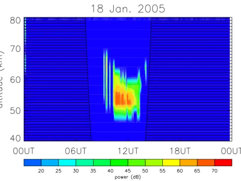
10

In Fig. 1 we show a typical isolated lower mesospheric echo observed by the Tromsø MF radar on 18 January 2005. Although a typical ILME, this date was chosen in partic-ular because it coincides with a PMWE event observed by a nearby VHF radar (L ¨ubken et al., 2006) and also in situ measurements of positive ion density fluctuations (Brattli et al., 2006). The echo is “isolated” because the radio wave above has been totally

15

absorbed by the ionized medium. Other echoes – partial reflections from refractive index structuring as the radio wave propagates through the lower ionosphere – have been excluded as being “normal”. By using signals from all altitudes and times we are able to construct the altitude profile of ε’ as shown in Fig. 2. In Fig. 2, the monthly mean profile (i.e. for January 2005) and its associated standard deviation, the latter

20

to be interpreted as the monthly variability, are shown by the black line and horizontal bars; the red line is the mean profile for 18 January, and the ochre region represents the variability; the numbers appearing to the right of the profiles give the numbers of 5-minute profiles comprising the daily average value at each height. We define a sig-nificant degree of turbulence to be wherever the mean profile for the day in question

25

exceeds the monthly mean plus one standard deviation. We can see that this is the case for measurements at 73 and 76 km (marginal at 70 and 79 km). One should note

(6)

ACPD

that the absolute values for estimates of turbulent energy dissipation rate using radar and in situ measurements should probably not be compared; nevertheless the radar method indicates larger upper limits for ε than usual in the very same altitude region as Brattli et al. (2006) report turbulence parameterized by lower limits for ε. At least on 18 January 2005, there is a degree of qualitative agreement between our method of

5

identifying enhanced turbulence and the more direct in situ method.

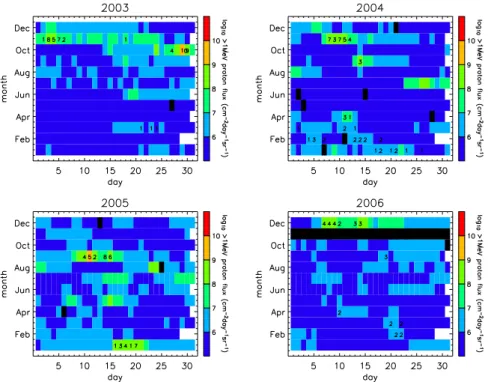
The information in Fig. 3 is, to some degree a repetition of that presented earlier by Hall et al. (2006), but only for the years 2003–2006 inclusive and with the 2006 re-sults being new. In the panels of the figure each day of the year can be identified by a large colour-coded pixel and numbers written over these pixels indicate the number

10

of hours of ILME during that day. “Black” days have no data. Essentially common to all days (with isolated, presumably spurious, exceptions) is that ILME are not observed unless the >1 MeV proton flux exceeds 106cm−2_day−1_sr−1_{and in the winter half of the}

year. Moreover, longer sequences of ILME are often associated with extended periods of larger fluxes (e.g. >107cm−2

day−1

sr−1

). Although observed short-lived instances

15

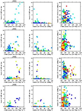
of ILME could be due to particularly energetic auroral precipitation, enhanced proton fluxes may, in general, be regarded as a necessary condition. Fig. 4 is a new repre-sentation of the information in Fig. 3 and including the ∆ε’ results described earlier. Since we have no a priori reason to examine any specific altitude, we have determined the median of ∆ε’ over the altitude interval 61–91 km. Several altitude intervals were

20

tested along with means instead of medians and the results are not shown here: using medians excludes spuriously large values and the chosen altitude interval covers the preferred PMWE and PMSE heights and yields a substantial number of data points. For each of the years 2003–2006 inclusive (arranged top to bottom) there are 3 pan-els: (i) hours of ILME per day as a function of >1MeV proton flux vs., (ii) hours of ILME

25

per day as a function of median ∆ε’ from the height interval 61–91 km, and (iii) median ∆ε’ as a function of >1 MeV proton flux (arranged left to right). The scatter plots are colour coded such that blues are winter days, reds are summer days, orange-yellow are early and late summer, and cyan-green are early and late winter. The first column

(7)

ACPD

essentially shows the same information as in Fig. 3, i.e. that the threshold for there being ILME (short-lived echoes of <1 h of ILME per day are included along the bottom axis) is approximately 106cm−2

day−1

sr−1

and fluxes of over 107cm−2

day−1

sr−1

are generally required for ILME events of more than 2 h per day. Furthermore the absence of yellow/orange/red symbols for >1 h per day events demonstrates ILME to be a

win-5

ter phenomenon. The second column simply illustrates a lack of correlation between enhanced turbulence and ILME: the majority of non-zero turbulence enhancements, at least as identified by the median of ∆ε’ from the height interval 61–91 km are not associated with ILME and there is no evidence whatsoever for strong turbulence giving rise to long ILME sequences. The third column attempts to identify any relationship

10

between enhanced proton flux and enhanced turbulence, but does not offer an unam-biguous answer. Enhancements in turbulence are caused by a variety of mechanisms which results in a spread of points in the figure. We cannot exclude the possibility that proton precipitation may affect turbulence generation, for example by modification of the temperature structure and we shall address this forthwith.

15

3 Discussion

The formats of Figs. 3 and 4 have been chosen to provide visual qualitative assess-ments of any correlations between ILME, proton flux and turbulence. The relation or rather dependence of ILME on enhanced proton flux has already been established by Hall et al. (2006) and the presence of ILME (a medium frequency radar phenomenon)

20

seems indicative of conditions conducive to PMWE observation by VHF radar. In the absence of any clear relation between turbulence and ILME, we have not deemed it necessary to attempt a quantitative correlation analysis between these parameters. At the same time it is not obvious that enhanced proton precipitation capable of pene-trating into the lower mesosphere and conceivably modifying the temperature structure

25

should not influence turbulence production. Given that enhanced proton fluxes can never be the sole causes of enhanced turbulence, we should expect the considerable

(8)

ACPD

spread in points in the 3rd column of Fig. 4. Nevertheless, one might perceive a sug-gestion of a weak dependence of ∆ε’ on proton flux, particularly in 2004 and 2006. Although this is material for a study in itself we can examine some known ILME/PMWE periods in more detail.

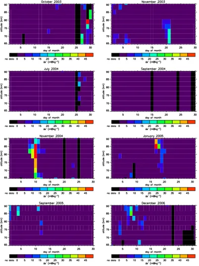
We have selected 8 months featuring enhanced proton fluxes from the 4 years of data

5

portrayed in Fig. 3 and have plotted ∆ε’ as a function of day and height (Fig. 5). Rather than make visually attractive contour plots, we have colour-coded day-wide 3 km high rectangles according to the actual ∆ε’. From an examination of these selected periods combined with the proton flux information from Fig. 3, we note the following:

1. 2003 October and November. Proton fluxes were relatively large from 14 October

10

until the end of November. Turbulence on 15 October corresponds to an isolated day with ∼107cm−2

day−1

sr−1

proton flux, but the increased fluxes on 23 October did not result in increased turbulence. All days during the Halloween event at the end of October featured increased turbulence. All days in November featuring enhanced turbulence corresponded to large proton fluxes, but not vice versa.

15

2. 2004. In July proton fluxes were enhanced from 23 to the end of the month with corresponding turbulence enhancements on 26 and 28. In mid-September en-hanced proton fluxes (inducing IMLE) failed to enhance turbulence. In November fluxes exceeded 107cm−2_day−1_sr−1 _{between 7 and 13 (ILME on 8–12) and}

tur-bulence was correspondingly enhanced on 8–13.

20

3. 2005. In January proton fluxes exceeded 106cm−2_day−1_sr−1 _{during the whole}

month and exceeded 107cm−2

day−1

sr−1

on 16–22; isolated turbulence enhance-ments occurred on 4 and 8 and there was a more general enhancement in the period 17–20. In September proton fluxes exceeded 107cm−2_day−1_sr−1_{on 8–17}

(ILME on several of these days) but turbulence was only enhanced on 11 and 12.

25

No outstanding proton fluxes characterize 1 and 4 September when turbulence was also enhanced.

(9)

ACPD

4. 2006. Proton fluxes were elevated during much of December, but particularly in the period 7–22; enhanced turbulence was seen on 6–13 (also when ionisation was sufficient for ILME).

Turbulent intensity (recall that it is identified here by instances where the estimated energy dissipation rate at a given height and day exceeds the corresponding monthly

5

mean plus one standard deviation) may be temporarily and locally enhanced by a vari-ety of mechanisms including wind shear, tropospheric forcing of gravity waves, changes in gravity wave filtering, convective instability etc. Enhancements in turbulence may therefore occur irrespective of high proton flux events. It is a difficult task to isolate enhancements which are in some way caused by proton precipitation but all the same,

10

it is difficult to dismiss the simultaneity of large proton fluxes and significant ∆ε’ as co-incidental. Jackman et al. (2007) have reported how a solar proton event, specifically October-November 2003, can cause ozone depletion and thus a cooling of the upper stratosphere and lower mesosphere and at the same time Joule heating of the up-per mesosphere. These effects were predicted to be most pronounced in the summer

15

hemisphere (lower mesosphere cooling by up to 2.5K and upper mesosphere heating by up to 4 K), but that the winter hemisphere sunlit atmosphere is not affected cannot be precluded. Detailed modelling will be required to investigate how the temperature structure changes caused by stratospheric cooling and upper mesospheric heating will affect gravity wave (GW) propagation into the mesosphere and stability. Qualitatively

20

though, an increase in the lapse rate in the lower/ middle mesosphere would encourage convective instability while decreasing the lapse rate near the mesopause would en-courage gravity wave saturation, and the whole scenario is compatible with an increase in turbulence.

We can thus both summarize the probable ILME mechanism and hypothesize a

pos-25

sible PMWE mechanism:

1. Solar proton events → deeper ionisation in polar regions during daylight → larger non-deviative absorption in winter → echoes at MF having the appearance of

(10)

ACPD

layers: ILME

2. Solar proton events → destruction of ozone combined with Joule heating modifies temperature profile → increased GW saturation, convective instability and possi-bly GW flux → more turbulence → ionisation + turbulence give rise to echoes at VHF: PMWE

5

4 Conclusions

While there is a clear correlation between enhanced solar proton precipitation and ILME occurrence (and hence, presumably, PMWE), there is no evidence for correla-tion between turbulent intensity and ILME. We do, on the other hand, find evidence for enhanced turbulence generation associated with enhanced proton flux. Obviously,

10

turbulence can be caused by a variety of atmospheric conditions, so finding enhanced turbulence when there is only normal proton flux is no surprise, and similarly large proton fluxes do not necessarily generate turbulence. Nevertheless large proton fluxes indeed appear to coincide with turbulent energy dissipation rates in excess of monthly averages. A full investigation of the mechanism for this is outside the scope of this

15

study but meanwhile our results provide a basis for investigating whether turbulence is a prerequisite for PMWE.

References

Belova, E., Kirkwood, S., Ekeberg, J., Osepian, A., H ¨aggstr ¨om, I., Nilsson, H., and Rietveld, M.: The dynamical background of polar mesosphere winter echoes from simultaneous

20

EISCAT and ESRAD observations, Ann. Geophys., 23, 1239–1247, 2005,

http://www.ann-geophys.net/23/1239/2005/.

Birch, M. J., Hargreaves, J. K., Senior, A., and Bromage, B. J. I.: Variations in cutoff latitude during selected solar energetic proton events, J. Geophys. Res., 110, A07221, doi:10.1029/2004JA010833, 2005.

(11)

ACPD

Brattli, A., Blix, T. A., Lie-Svendsen, Ø. , Hoppe, U.-P. , L ¨ubken, F.-J. , Rapp, M. , Singer, W. , Lat-teck, R., and Friedrich, M.: Rocket measurements of positive ions during polar mesosphere winter echo conditions, Atmos. Chem. Phys., 6, 5515–5524, 2006,

http://www.atmos-chem-phys.net/6/5515/2006/.

Hall, C. M.: The Ramfjormoen MF radar (69◦_{N, 19}◦_{E): Application development 1990-2000, J.}

5

Atmos. Solar-Terr. Phys., 63, 171–179, 2001.

Hall, C. M., Meek, C. E., and Manson, A. H.: Turbulent energy dissipation rates from the University of Tromsø/University of Saskachewan MF radar, J. Atmos Solar Terr. Phys, 60, 437–440, 1998.

Hall, C. M., Meek, C. E. and Manson, A. H., and Nozawa, S.: Isolated lower mesospheric

10

echoes seen by medium frequency radar at 70◦_{N, 19}◦_{E, Atmos. Chem. Phys., 6, 5307–}

5314, 2006,http://www.atmos-chem-phys.net/6/5307/2006/.

Hall, C. M., Aso, T., and Tsutsumi, M.: Atmospheric stability at 90 km, 78◦_{N, 16}◦_{E, in press}

Earth Planets Space, 2007.

Hargreaves, J. K.: The solar-terrestrial environment, 420pp., Cambridge University Press,

15

Cambridge, UK, 1992.

Hargreaves, J. K. and Birch, M. J.: On the relations between proton influx and D-region electron densities during the polar-cap absorption event of 28–29 October 2003, Ann. Geophys., 23, 3267–3276, 2005,http://www.ann-geophys.net/23/3267/2005/.

Jackman, C. H., Roble, R. G., and Fleming, E. L.: Mesospheric dynamical changes induced

20

by the solar proton events in October–November 2003, Geophys. Res. Lett., 34, L04812, doi:10.1029/2006GL028328, 2007.

Kirkwood, S. C., Barabash, V., Belova, E., Nilsson, H., Rao, T. N., Stebel, K., Osepian, A., and Chilson, P. B.: Polar mesosphere winter echoes during solar proton events, Adv. Polar Upper Atmos. Res., 16, 111–125, 2002.

25

L ¨ubken, F.-J., Strelnikov, B., Rapp, M., Singer, W., Latteck, R., Brattli, A., Hoppe, U.-P., and Friedrich, M.: The thermal and dynamical state of the atmosphere during polar meso-sphere winter echoes, Atmos. Chem. Phys., 6, 13–24, 2006,

http://www.atmos-chem-phys.net/6/13/2006/.

Zeller, O., Zecha, M., Bremer, J., Latteck, R., and Singer, W.: Mean characteristics of

meso-30

spheric winter echoes at mid- and high latitudes, J. Atmos. Solar Terr. Phys., 68, 1087–1104, doi:10.1016/j.jastp.2006.02.015, 2006.

(12)

ACPD

(13)

ACPD

Fig. 2. Estimates of turbulent energy dissipation rate, denoted by ε’ for 18 January 2005.

The black line with associated variability bars shows the January 2005 mean and standard deviation; the red line and ochre shaded region show the mean profile for 18 January and its standard deviation respectively; the numbers to the right of the profiles indicate the numbers of 5-min samples at each height comprising the mean profile for 18 January. Turbulence is deemed to be significantly enhanced over the monthly mean wherever the day-average (red) profile is greater than the monthly mean plus one standard deviation (black lines).

(14)

ACPD

Fig. 3. Yearly tables of month versus day for Tromsø the period 2003–2006 inclusive. For days

when ILME were detected (according to the criteria of Hall et al., 2006) the total number of hours are indicated. The background colours indicate >1 MeV proton fluxes. Black indicates whenever the Tromsø MF radar experienced operation problems of some kind.

(15)

ACPD

Fig. 4. Scatter plots for the period 2003–2006 (top to bottom) inclusive. Leftmost column: hours

of ILME per day as a function of >1 MeV proton flux vs.; centre column: hours of ILME per day as a function of median ∆ε’ from the height interval 61–91 km; rightmost column: median ∆ε’ as a function of >1 MeV proton flux (arranged left to right). The scatter plots are colour coded such that blues are winter days, reds are summer days, orange-yellow are early and late summer, and cyan-green are early and late winter.

(16)

ACPD

Fig. 5. The metric ∆ε’ as a function of height and day for selected months during which notable