Multiculturalism and Growth: Skill-Specific Evidence from the Post-World War II Period

HAL Id: halshs-01425462

https://halshs.archives-ouvertes.fr/halshs-01425462

HAL is a multi-disciplinary open access archive for the deposit and dissemination of sci-entific research documents, whether they are pub-lished or not. The documents may come from teaching and research institutions in France or abroad, or from public or private research centers.

L’archive ouverte pluridisciplinaire HAL, est destinée au dépôt et à la diffusion de documents scientifiques de niveau recherche, publiés ou non, émanant des établissements d’enseignement et de recherche français ou étrangers, des laboratoires publics ou privés.

Frédéric Docquier, Riccardo Turati, Jérôme Valette, Chrysovalantis Vasilakis

To cite this version:

Frédéric Docquier, Riccardo Turati, Jérôme Valette, Chrysovalantis Vasilakis. Multiculturalism and Growth: Skill-Specific Evidence from the Post-World War II Period. 2017. �halshs-01425462�

C E N T R E D'E T U D E S E T D E R E C H E R C H E S S U R L E D E V E L O P P E M E N T I N T E R N A T I O N A L

SÉRIE ÉTUDES ET DOCUMENTS

Multiculturalism and Growth: Skill-Specific

Evidence from the Post-World War II Period

Frédéric Docquier, Riccardo Turati, Jérôme Valette, Chrysovalantis Vasilakis

Études et Documents n° 24

December 2016

To cite this document:

Docquier F., Turati R., Valette J., Vasilakis C. (2016) “Multiculturalism and Growth: Skill-Specific Evidence from the Post-World War II Period”, Études et Documents, n° 24, CERDI.

http://cerdi.org/production/show/id/1838/type_production_id/1

CERDI

65 BD. F. MITTERRAND

63000 CLERMONT FERRAND – FRANCE

TEL.+33473177400

FAX +33473177428

2

The authors Frédéric Docquier

FNRS & IRES, Université Catholique de Louvain (Belgium), and FERDI (France). E-mail: frederic.docquier@uclouvain.be

Riccardo Turati

IRES, Université Catholique de Louvain (Belgium). E-mail: r.turati@uclouvain.be

Jérôme Valette

CERDI – Clermont Université, Université d’Auvergne, UMR CNRS 6587, 65 Bd F. Mitterrand, 63009 Clermont-Ferrand, France.

E-mail: jerome.valette@udamail.fr

Chrysovalantis Vasilakis

IRES, Université Catholique de Louvain (Belgium) and Bangor Business School (United Kingdom). E-mail: chvasi-lakis@gmail.com

Corresponding author: Jérôme Valette

This work was supported by the LABEX IDGM+ (ANR-10-LABX-14-01) within the program “Investissements d’Avenir” operated by the French National Research Agency (ANR).

Études et Documents are available online at: http://www.cerdi.org/ed

Director of Publication: Vianney Dequiedt Editor: Catherine Araujo Bonjean

Publisher: Mariannick Cornec ISSN: 2114 - 7957

Disclaimer:

Études et Documents is a working papers series. Working Papers are not refereed, they constitute

research in progress. Responsibility for the contents and opinions expressed in the working papers rests solely with the authors. Comments and suggestions are welcome and should be addressed to the authors.

3

Abstract

This paper empirically revisits the impact of multiculturalism (as proxied by indices of birthplace diversity and polarization among immigrants, or by epidemiological terms) on the macroeconomic performance of US states over the 1960-2010 period. We test for skill-specific effects of multiculturalism, controlling for standard growth regressors and a variety of fixed effects, and accounting for the age of entry and legal status of immigrants. To identify causation, we compare various instrumentation strategies used in the existing literature. We provide converging and robust evidence of a positive and significant effect of diversity among college-educated immigrants on GDP per capita. Overall, a 10% increase in high-skilled diversity raises GDP per capita by 6.2%. On the contrary, diversity among less educated immigrants has insignificant effects. Also, we find no evidence of a quadratic effect or a contamination by economic conditions in poor countries.

Keywords

Immigration, Culture, Birthplace diversity, Growth.

JEL Codes

F22, J61

Acknowledgment

We are grateful to Simone Bertoli, Jean-Louis Combes, Oded Galor and Hillel Rapoport for helpful comments. This paper has also benefited from discussions at the SEPIO Workshop on Cultural Diversity (Paris, May 2016), at the Workshop on “The Importance of Elites and their Demography for Knowledge and Development” (Louvain-la-Neuve, June 2016), at the XII Migration Summer School at EUI (Florence, July 2016) and at the 7th International Conference "Economics of Global Interactions: New Perspectives on Trade, Factor Mobility and Development" (Bari, September 2016). The first author is grateful for the financial support from the Fonds spéciaux de recherche granted by the National Fund for Scientific Research (FNRS grant n. 14679993).

1 Introduction

Patterns of international migration to industrialized countries have drastically changed since World War II (WW2). On average, the share of foreigners in the population of high-income countries increased from 4.9 to 11.7% between 1960 and 2010 (Özden et al., 2011).1 _This phenomenon has similarly affected the United States (from 5.4 to 13.6%), the members of the European Union (from 3.9 to 12.2%), Canada and Australia (from 15 to 22%). In addition, this change has been predominantly driven by immigration from developing countries; the share of South-North immigrants in the population of high-income countries increased from 2.0 to 8.7% in half a century.2 _{This growing inflow of people coming from geographically,} economically and culturally distant countries raises specific issues, as it has conceivably brought different skills and abilities, but also different social values and norms, or different ways of thinking. Although a large body of literature has focused on the size and skill structure of immigration flows, the macroeconomic effects of multiculturalism, as well as the channels through which they materialize, are still uncertain.

This paper empirically revisits the impact of multiculturalism on the macroeconomic per-formance of US states (proxied by their level of GDP per capita) in the aftermath of WW2. Our analysis combines three distinctive features. First, we rely on panel data available for a large number of regions over a long period. Our sample covers all US states over the 1960-2010 period in ten-year intervals. The use of panel data allows us to better deal with unobserved heterogeneity and endogeneity issues. This is crucial because economic prosper-ity and the degree of diversification of production are likely to attract people from different cultural origins. Multiculturalism is thus likely to respond to changes in the economic envi-ronment (see Alesina and La Ferrara (2005)), implying that causation is hard to establish in a cross-sectional setting. To control for unobserved heterogeneity and reverse causation biases, our paper uses a great variety of geographic and time fixed effects, and combines various instrumentation strategies that have been used in the existing literature. Second, we system-atically investigate whether the economic effect of multiculturalism is heterogeneous across skill groups. The costs and benefits from multiculturalism are likely to vary with the levels

1_{This is not the case in developing countries, where the average immigration rate has decreased by half}

(from 2.3 to 1.1%) since 1960. Although the worldwide stock of international migrants increased from 91.6 to 211.2 million, the worldwide share of international migrants has been fairly stable since 1960, fluctuating around 3%. This is only 0.3 percentage points above the level observed in the early 20th century (McKeown, 2004).

2_{Immigration from developing countries accounts for 98% of the 1960-2010 rise in immigration to}

high-income countries, for 80% in the European Union, for 120% in the United States, and for 150% in Australia and Canada. Trends in immigration to the US are presented in the supplementary appendix.

of task complexity and interaction between workers; meanwhile, high-skilled and low-skilled immigrants are likely to heterogeneously propagate social values and norms across borders. We account for this by using skill-specific measures of multiculturalism. In addition, taking advantage of the availability of microdata, we compute our indices of multiculturalism for different groups of immigrants (by age of entry or by legal status). Third, we jointly test for different technologies and/or channels of transmission. We follow Alesina et al. (2016) and proxy multiculturalism with indices of birthplace diversity, measuring the probability that two randomly-drawn individuals from a particular state have different countries of birth. In alternative specifications, we allow for non-linear effects, and include epidemiological (or contamination) forces, as well as an index of birthplace polarization of the workforce.

Our paper belongs to a recent and increasing strand of literature which considers that culture can be a feature which differentiates individuals in terms of their attributes, that this differentiation may have positive or negative effects on people’s productivity, and that culture is affected by the country of birth (which determines the language and social norms individuals were exposed to in their youth, the education system, etc.). On the one hand, homogenous people are more likely to get along well, which implies that multiculturalism may reduce trust or increase communication, cooperation and coordination costs. Moreover, birthplace diversity can also be the source of epidemiological effects, as argued by Collier (2013) and Borjas (2015): by importing their “bad” cultural, social and institutional models, migrants from developing countries may contaminate the entire set of institutions in their country of adoption, levelling the world distribution of technological capacity downwards. On the other hand, cultural diversity also enhances complementarities across diverse pro-ductive traits, stimulating innovations and the collective capacity to solve problems; a more diverse group is likely to spawn different cultures with various solutions to the same problem. Evidence of such costs and benefits has been found in micro studies. For example, Parrotta et al. (2014) investigate the effect of different forms of diversity (by education, age group, and nationality) on the productivity of Danish firms, using a matched employer-employee database. They find a negative effect of workers’ diversity by nationality on productivity. On the contrary, Ozgen et al. (2014) find that birthplace diversity increases the likelihood of innovations using Dutch firm-level survey data, and Boeheim et al. (2012) find a positive effect of diversity on productivity using Austrian data. Finally, Kahane et al. (2013) find a positive effect of diversity on hockey team performance using data from the NHL (the North American National Hockey League).

for interdependencies between firms, industries, and/or regions. Existing studies have iden-tified significant and positive effects of multiculturalism on comparative development and on disparities in economic performance across modern societies.3 _{Ottaviano and Peri (2006) use} US data by metropolitan area over the 1970-1990 period. In their (log of) wage regressions, the coefficient of diversity varies between 0.7 and 1.5. Ager and Brückner (2013) use US data by county during the 1870-1920 period: the coefficient of diversity in the output per capita regressions varies between 0.9 and 2.0. In these two studies, endogeneity issues are solved by using a shift-share method, i.e. computing the diversity index on the basis of predicted immigrant stocks. More precisely, the change in immigration to a region is pre-dicted as the product of the global change in immigration to the US by the regional share in total immigration in the initial year. A more recent study accounting for the education level of immigrants is that of Alesina et al. (2016); it is the most similar to ours. They use cross-sectional data on immigration stocks by education level for a large set of countries in the year 2000, and develop a pseudo-gravity first-stage model to predict migration stocks and birthplace diversity indices. They also identify a positive effect of birthplace diversity in countries with GDP per capita above the median, and a stronger effect for diversity among college-educated workers. The effect of diversity on the log of GDP per capita is around 0.1 when computed on low-skilled workers, while the effect of diversity among the highly skilled varies between 0.2 and 0.3. Similarly, Suedekum et al. (2014) use annual German data by region from 1995 to 2006. Over this short period, they find a lower effect of diversity on the log of German wages (about 0.1 for diversity among high-skilled foreigners, and 0.04 for diversity among the low skilled) when fixed effects and IV methods are used.

Our empirical analysis relies on high-quality US census data by state over the 1960-2010 period. The choice of this period is guided by the 1965 amendments to the Immigration and Nationality Act, which led to an upward surge in U.S. immigration and diversity (as in Ottaviano and Peri (2006)). Birthplace diversity is almost perfectly correlated with the state-wide proportion of immigrants, which has increased threefold since 1960 in all skill groups. It is thus statistically impossible to disentangle the effects of birthplace diversity from those of the size of immigration. For this reason, we opt for a benchmark model that includes the immigration rate and a birthplace diversity index pertaining to the immigrant

3_{On the contrary, the empirical literature on ethnic and linguistic fractionalization identifies negative}

effects on economic growth (at least in developing countries). As for Ashraf and Galor (2013) (2013), they use the concept of genetic diversity (capturing within-group heterogeneity in genomes between regions), and find that it explains about 25% of the different development outcomes (as proxied by population density) around the year 1500, i.e. before the age of mass migration. They identify an inverted-U shape relationship, suggesting that there is an optimal level of diversity for economic development.

population. In line with Alesina et al. (2016) and Suedekum et al. (2014), we find that diversity among college-educated immigrants is positively associated with the level of GDP per capita; however, diversity among less educated immigrants has insignificant (or weakly significant) effects. Another remarkable result is that the estimated coefficient is divided by four when geographic and year fixed effects are included. Overall, a 10% increase in diversity among college-educated immigrants raises GDP per capita by 6.2%. These results are robust to the exclusion of some census years, to the set of US states included in the sample, and to the measurement of diversity. The results hold true when we eliminate states with the greatest or smallest levels of immigration share, states located on the Mexican border, and states with the lowest proportions of immigrants. They are also valid when we exclude undocumented immigrants and those who arrived in the US at a young age. Importantly, we find no evidence of an inverted-U shaped relationship a la Ashraf and Galor (2013), or of a negative epidemiological effect a la Collier (2013) and Borjas (2015). On the contrary, we find that immigrants from richer countries have a smaller effect on GDP per capita than those from poorer countries; we interpret this as a confirmation that diversity among college-educated immigrants matters more than the economic conditions at origin. Finally, birthplace diversity is negatively correlated with the index of polarization in the immigrant population. If, instead of diversity, a high-skilled polarization index is used, we obtain a highly significant and negative effect on GDP per capita.

To address endogeneity issues, we consider two instrumentation strategies that have been used in the related literature. The first one is a shift-share strategy a la Ottaviano and Peri (2006) which includes the predicted diversity indices based on total US immigration stocks by country of origin, and the bilateral state shares observed in 1960. The second strategy consists in instrumenting diversity indices, using the immigration predictions of a pseudo-gravity regression that include interactions between year dummies and the geographic distance between each country of origin and each state of destination (in line with Feyrer (2009) or Alesina et al. (2016)). In both cases, diversity among college-educated migrants remains highly significant, while diversity among the less educated is insignificant or weakly significant. In the preferred specification, the coefficient of high-skilled diversity is equal to 0.616. At first glance, this seems important because the average diversity index among college-educated immigrants equals 0.937 in 2010; hence, increasing diversity from zero to 0.937 increases GDP per capita by 58%. However, in 2010, the high-skilled diversity index ranges from 0.797 to 0.976. If all US states had the same level of diversity as the District of Columbia (0.976), the average GDP per capita of the US would be 2.33% larger, the

coefficient of variation across states would be 2.37% smaller, and the Theil index would decrease by 3.45%, only. By comparison, if all US states had the same average level of human capital as the District of Columbia, the average GDP per capita of the US would be 8.32% larger, the coefficient of variation across states would be 9.77% smaller, and the Theil index would decrease by 16.06%. Although diversity has non-negligible effects on cross-state disparities, its macroeconomic implications are rather limited.4 _{We reach the same conclusion} when using the longitudinal dimension of the data. The US-state average level of diversity among college-educated migrants increased by 7 percentage points between 1960 and 2010; this explains a 3.5% increase in macroeconomic performance (i.e. only one fiftieth of the total change in the US level of GDP per capita).

The remainder of the paper is organized as follows. Section 2 describes our main diversity measures and documents the global trends in cultural diversity in the aftermath of WW2. Section 3 describes our empirical strategy. The results are discussed in Section 4. Finally, Section 5 concludes.

2 Diversity in the Aftermath of WW2

Following Ottaviano and Peri (2006), Ager and Brückner (2013), Suedekum et al. (2014) and Alesina et al. (2016), we consider that the cultural identity of individuals is mainly determined by their country of birth. The rationale is that the competitiveness of modern-day economies is closely linked to the average level of human capital of workers and to the complementarity between their skills. Workers originating from different countries were trained in different school systems and are more likely to bring complementary skills, cognitive abilities and productive traits. In our benchmark model, our key explanatory variable is an index of birthplace diversity (or birthplace fractionalization), which can be computed for each US state and for the high-skilled and low-skilled populations separately. In subsection 2.1, we first define various measures of birthplace diversity, establish links between them, and discuss their statistical correlation with the average immigration rate. In subsection 2.2, we then document the global US trends in cultural diversity observed in the aftermath of WW2.

4_{The GDP per capita of Hawaii (diversity index of 0.797) would be 11.66% larger if Hawaii had the same}

diversity index as the District of Columbia; the difference in high-skilled diversity explains about 4.7% of the total income gap between these two states in 2010.

2.1 The Birthplace Diversity Index

In line with existing studies, we first define a Herfindahl-Hirschmann index of birthplace diversity, T DS

r,t, which can be computed for the skill group S = (L, H, A) (L for the low skilled, H for the high skilled, and A for both groups), for each region r = (1, ..., R) and for each year t = (1, ..., T ). Our index measures the probability that two randomly-drawn individuals from the type-S population of a particular region originate from two different countries of birth. As shown by Alesina et al. (2016) in a cross-country setting, the birthplace diversity index is poorly correlated with genetic or ethnolinguistic fractionalization indices. The index is written:

T D_r,tS = I X i=1 k_i,r,tS (1 k_i,r,tS ) = 1 I X i=1 (k_i,r,tS )2, (1) where kS

i,r,tis the share of individuals of type S, born in country i, and living in region r, in the type-S resident population of the region at year t. Computing the birthplace diversity index requires collecting panel data on the structure of the population by region of destination, by country of origin, and by education level. Our sample includes all US states (including the District of Columbia) between 1960 and 2010 in ten-year intervals, i.e. r = (1, ..., 51) and t = (1960, ..., 2010). Our choice to conduct the analysis at the state level is guided by the availability of long-term data series on macroeconomic performance, and by the comparability with cross-country results. We identify a common set of 195 countries of origin, including the US as a whole.5

Building on Alesina et al. (2016), the additive decomposition of the diversity index al-lows to distinguish between the Between and the Within components of the diversity index, T DS

r,t = BDr,tS + W DSr,t. On the one hand, the Between component BDr,tS measures the prob-ability that a randomly-drawn pair of type-S residents includes a native and an immigrant, irrespective of where the immigrant comes from:

BD_r,tS = 2k_r,r,tS (1 kS_r,r,t). On the other hand, the residual Within component W DS

r,t measures the probability that a randomly-drawn pair of type-S residents includes two immigrants born in two different countries:

5_{We disregard heterogeneity between US natives born in different states (e.g. a Texan native is considered}

W D_r,tS = I X

i6=r

k_i,r,tS (1 k_i,r,tS k_r,r,tS ).

In the US context, the evolution of the birthplace diversity index among residents is almost totally driven by the change in the Between component of diversity, BD_{r,t, which}S only depends on the proportion of immigrants. The median share of the Between component in total diversity, BDA

r,t/T DAr,t, equals 0.98% and its quartiles are equal to 0.92% and 0.97%. Similar findings are found for the low-skilled and high-skilled populations. Consequently, birthplace diversity in group S is almost perfectly correlated with the region-wide proportion of immigrants.6 _{On average, the Pearson correlation between T D}S

r,t and the total share of immigrants in the population, mS

r,t = (1 kSr,r,t), equals 0.99 for all S. It is thus impossible to statistically disentangle the effects of diversity from those of immigration. For this reason and in line with existing works, our empirical specification distinguishes between the size of immigration and the variety of immigrants.

To capture the variety effect, we start from the Within component of the diversity index. The Within component can be expressed as the product of the square of the immigration rate (the probability that two randomly-drawn individuals are immigrants) by an index of diversity among immigrants, MDS

r,t. The latter measures the probability that two randomly-drawn immigrants from region r originate from two different countries of birth. We have:

W D_r,tS = (1 kS_r,r,t)2M D_r,tS (2) = (1 kS_r,r,t)2X i6=r bkS i,r,t(1 bkSi,r,t), where bkS

i,r,t = ki,r,tS /(1 kr,r,tS ) is the share of immigrants from origin country i in the total immigrant population of region r. Contrary to the total index of diversity and to its Between and Within components, the correlation between MDS

r,t and the total immigration rate, mSr,t, is small (on average, -0.19). This allows us to simultaneously include these two variables in the same regression without fearing collinearity problems.

6_{This is shown in Table A4 in the Appendix, which provides correlations between diversity indices, and}

2.2 Diversity in US States

Population data at the state level for the US are available from the Integrated Public Use Microdata Series (IPUMS). IPUMS data are drawn from the federal census of the American Community Surveys. For each census year, they allow characterizing the evolution of the American population by country of birth, age, level of education, and year of arrival in the US, among others. We extracted the data from 1960 to 2010 in ten-year intervals, using the 1% census sample for the years 1960 and 1970, the 5% census sample for the years 1980, 1990 and 2000, and the American Community Survey (ACS-1%) sample for the year 2010. Regarding the origin countries of immigrants, we consider the full set of countries available in 2010, although some of them had no legal existence in the previous census years. Hence, for the years 1960 to 1990, data for the former USSR, former Yugoslavia and former Czechoslovakia are split using the country shares observed in the year 2000. In addition, we treat five pairs of countries as a single entity; this is the case of East and West Germany, Kosovo, Serbia and Montenegro, North and South Korea, North and South Yemen, and Sudan and South Sudan. Finally, we allocate individuals with a non-specified (or an imperfectly specified, respectively) country of birth proportionately to the country shares in the US population (or to the country shares in the US population originating from the reported region, respectively).

In our benchmark regressions, we restrict our micro sample to all individuals aged 16 to 64, who are likely to affect the macroeconomic performance of their state of residence. We distinguish between two skill groups. Individuals with at least one year of college are classified as highly skilled, whereas the rest of the population is considered as low skilled. We define as US natives all individuals born in the US or in US-dependent territories such as American Samoa, Guam, Puerto Rico, the US Virgin Islands and other US possessions. Other foreign-born individuals are referred to as immigrants.

In alternative regressions, we only consider immigrants who arrived in the US after a certain age, or immigrants who are likely to have a legal status. As for the age-of-entry correction, we sequentially eliminate immigrants who arrived before the age of 5, 6, ... , 25. In order to proxy the number of undocumented immigrants, we follow the “residual method-ology” described in Borjas (2016), and use information on the respondents’ characteristics (such as citizenship, working sector, occupation, whether they receive public assistance, etc.).

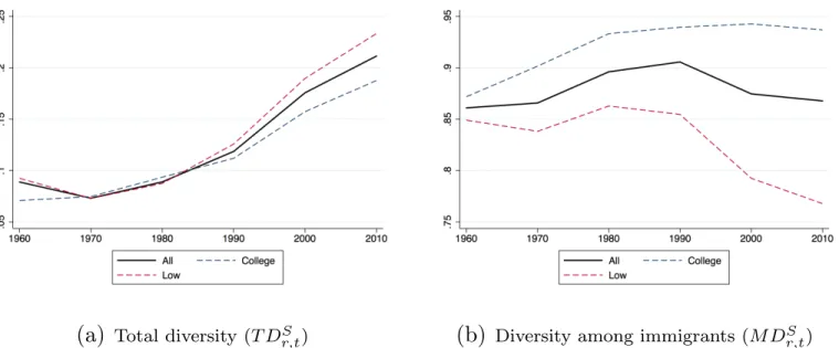
Figure 1: Trends in birthplace diversity in US states, 1960-2010

(a)

r,t)

(b)

Notes: Diversity among residents is defined as in Eq. (1), whereas diversity among immigrants is defined as in Eq. (2). Source: Authors’ elaboration on IPUMS data.

We use IPUMS data to identify the bilateral stocks and shares of international migrants, kS

i,r,t, in the population of each state r, by country of origin i and by education level S in the year t. We thus construct comprehensive matrices of "Origin ⇥ State ⇥ Skill" stocks and shares from 1960 to 2010 in ten-year intervals.7 _{Missing observations are considered} as zeroes, even if a positive number of immigrants is identified for an adjacent year.8 _The evolution of the average index of cultural diversity is described in Figure 1, whereas Figure 2 represents differences in the average level of diversity across US states.

Figure 1(a) describes the evolution of the birthplace diversity index computed for the resident population, T DS

r,t for all S, between 1960 and 2010. Looking at the average of all US states, the birthplace diversity index among residents increased from about 0.09 in 1960 to 0.21 in 2010, reflecting the general rise in immigration to the US. A large portion of this change occurred after 1990. Nevertheless, this average trend conceals important differences between US states and between skill groups. As far as cross-state differences are concerned, the number of immigrants drastically increased in states such as California

7_{We distinguish between 195 countries of birth and 50 US states plus the District of Columbia. The list}

of countries and states are provided in the Appendix A2, as well as descriptive statistics by state (see Table A3).

8_{The number of zeroes equals 33,145 out of a sample of 59,670 observations (55.5%). The missing values}

(+195%) or New York (+91%); on the contrary, the number of foreign-born individuals remained small and stable in other states such as Montana or Maine. Regarding differences between skill groups, changes in immigration rates were larger for the low skilled than for college graduates, particularly after the year 1980. This is mainly due to the large inflows of low-skilled Mexicans observed during the last three decades, which drastically affected the level of diversity in states located on the West Coast and along the US-Mexican border, as illustrated by Figure 2(a).

Second, Figure 1(b) describes the evolution of the diversity index computed for the im-migrant population, MDS

r,t for all S. It shows that on average, the level of diversity in the immigrant population varies across skill groups. Diversity among college-educated immi-grants has always been greater than diversity among the less educated. This might be due to the fact that college-educated migrants are less prone to concentrate in regions where large migration networks exist; they consider moving to more (geographically) diversified lo-cations. Differences between skill groups drastically increased after 1960. On the one hand, diversity among high-skilled immigrants increased during the sixties and seventies, possibly due to the the Immigration and Nationality Act of 1965. Changes have been smaller since 1980 despite the Immigration Act of 1990, which allocated 50,000 additional visas (in the form of a lottery) to people from non-typical origin countries. On the other hand, diversity among low-skilled immigrants has fallen since 1980. Again, the latter decline is mainly ex-plained by the large inflows of low-skilled Mexicans. Along the Mexican border and on the West Coast, the probability that two randomly-drawn immigrants were born in two different countries decreased as the share of Mexicans increased. This is also illustrated in Figure 2(b), which reveals important cross-state differences in the long-run average level of diversity among immigrants.

In sum, the evolution of diversity among immigrants varies across US states and over time. Figure A2 in the Appendix reveals that diversity among immigrants decreased in states located along the US-Mexican border and on the West Coast. A rise in diversity was observed in other states (such as Maine or Vermont). Our panel data analysis takes advantage of these intra-state and inter-state variations to identify a causal effect of diversity on macroeconomic performance.

Figure 2: Cross-state differences in birthplace diversity, 1960-2010 average index

(a) Diversity among residents (T DA

r,t)

(b)Diversity among immigrants (MDA

r,t)

Notes: Diversity among residents is defined as in Eq. (1), whereas diversity among immigrants is defined as in Eq. (2). The two maps present the average birthplace diversity observed between 1960 and 2010. Alaska and Hawaii are not represented. Source: Authors’ elaboration on IPUMS data.

3 Empirical Strategy

Our goal is to identify the effect of multiculturalism on the macroeconomic performance of US states.9 _{The level of macroeconomic performance is measured by the log of the Gross}

9_{In the supplementary Appendix, a complementary analysis is conducted on the 34 OECD member}

Domestic Product (GDP) per capita. In subsection 3.1, we present the benchmark specifica-tion in which multiculturalism is proxied by the skill-specific indices of birthplace diversity described in Section 2. In subsection 3.2, we consider alternative specifications for the trans-mission of cultural shocks, which can be tested jointly with birthplace diversity or separately. Subsection 3.3 discusses the two instrumentation strategies that we use to deal with endo-geneity issues. Finally, subsection 3.4 presents the data sources used to construct our control variables and instruments.

3.1 Benchmark Specification

Our benchmark empirical model features the log of GDP per capita as the dependent variable. In line with Ottaviano and Peri (2006), Ager and Brückner (2013), Suedekum et al. (2014) and Alesina et al. (2016), our specification is written:

log(yr,t) = 1M DSr,t+ 2mSr,t+ 0Xr,t+ r+ t+ "r,t, (3) where log(yr,t) is the log of GDP per capita in region r at year t, MDS

r,t is the type-S birthplace diversity among immigrants (proxy for the variety of immigrants), and mS

r,t is the proportion of immigrants in the working-age population of type S. The latter variable captures the other channels through which the level of immigration affects macroeconomic performance (e.g. labor market, fiscal or market-size effects). We opt for a static specification and assume that changes in diversity fully materialize within 10 years. This spares us from dealing with the endogeneity of the lagged dependent, an important issue in dynamic models with a short-panel dimension (Nickel, 1981).10

The coefficient 1 is our coefficient of interest. It captures the effect of multicultural-ism on macroeconomic performance. Using skill-specific measures of cultural diversity and immigration, S = (L, H, A), we can identify whether the level and significance of 1 vary across skill groups. We first estimate Eq. (3) using pooled OLS regressions, bearing in mind that such regressions raise a number of econometric issues that might generate inconsistent estimates. The key issue when using pooled OLS regressions is the endogeneity of the main

not report the educational structure of migration stocks. To capture skill-specific effects, we combine it with the 1990-2000 estimates of the bilateral proportion of college graduates provided in Artuc et al. (2015). The second drawback is that it relies on imputation techniques to fill the missing bilateral cells. Despite the lower quality of the data, our fixed-effect analysis globally confirms the results obtained for US states.

10_{Nevertheless, in Appendix Tables A9 and A10, we provide the results of dynamic GMM regressions with}

internal or external instruments, and with different lag structures. In these regressions, the lagged dependent is insignificant or weakly significant, which reinforces the credibility of our static benchmark specification. In addition, the effect of diversity is similar to that obtained in the static model.

variable of interest, the index of diversity. Endogeneity can be due to a number of reasons. These reasons include the existence of uncontrolled confounding variables causing both de-pendent and indede-pendent variables, the existence of a two-way causal relationship between these variables, or a measurement problem.

To mitigate the possibility of an omitted variable bias, the benchmark model includes a vector Xi,t of time-varying covariates. It includes the log of population, the log of the region-wide average educational attainment of the working-age population (as measured by the years of schooling or highest degree completed), and the log of the urbanization rate. In addition, our specification includes a full set of region and year fixed effects, r and t, which allows us to better account for unobserved heterogeneity (including initial conditions in 1960). To solve the reverse causation and measurement problems, we combine two methods of instrumental variables described in subsection 3.3.

3.2 Alternative Specifications

Our benchmark specification Eq. (3) assumes linear effects of the level of immigration and of the variety of immigrants on the log of GDP per capita. The literature on multicultural-ism suggests that the technology of transmission of cultural shocks can be different. Three alternative specifications are considered in the robustness analysis. 11

First, looking at the effect of genetic diversity on economic development, Ashraf and Galor (2013) and Ashraf et al. (2015) consider a quadratic specification, which allows them to identify an optimal level of diversity. In our context, cultural diversity may also induce costs and benefits, implying that its effect on macroeconomic performance could be better captured by an inverted-U shape relationship. We thus naturally extend our benchmark specification by adding the square of the birthplace diversity index.

Second, Ager and Brückner (2013) consider two measures of cultural diversity. The first one is our standard index of fractionalization; the second one is a measure of cultural polarization. The rationale is that a more polarized population can be associated with increased social conflict and a reduction in the quality and quantity of public good provision.

11_{The birthplace diversity index MD}S

r,t does not account for the cultural distance between origin and

destination countries. It assumes that all groups are culturally equidistant from each other. Another extension consists therefore in multiplying the probability that two randomly-drawn immigrants were born in two different countries by a measure of cultural distance between these two countries. For the latter, we use the database on genetic distance between countries, constructed by Spolaore and Wacziarg (2009). Genetic distance is based on blood samples and proxies the time since two populations had common ancestors. It is worth noticing that our results are robust to the use of an augmented diversity index and are reported in the supplementary Appendix.

In line with Montalvo and Reynal-Querol (2003) and Montalvo and Reynal-Querol (2005), the polarization index captures how far the distribution of a population is from the bimodal distribution. It is written: T P_r,tS = 1 I X i=1 0.5 kS i,r,t 0.5 !2 kS_i,r,t. (4)

Applied to the immigrant population, the index is maximized when there are two groups of immigrants which are of equal size (i.e. 50%). For US states, the polarization index exhibits a correlation of -0.89 with the fractionalization index. Hence, including these two variables in the same regression is risky. In our robustness checks, we thus consider alternative specifications in which the birthplace diversity index is replaced by a polarization index (MPS

r,t) computed for the type-S immigrant population (i.e. using bki,r,tS instead of ki,r,tS in Eq. (4)).

Third, another strand of the literature focuses on migration-induced transfers of norms, and tests for potential epidemiological or contamination effects. Transfers of norms from origin to destination countries have been examined by a limited set of studies.12 _Comparing the economic performance of US counties from 1850 to 2010, Fulford et al. (2015) show that the country-of-ancestry distribution of the population matters, and that the estimated effect of ancestry is governed by the sending country’s level of economic development, as well as by measures of social capital at origin (such as trust and thrift). Putterman and Weil (2010) study the effect of ancestry in a cross-country setting, and find that the ancestry effect is governed by a measure of state centralization in 1500. More recently, debates about the societal implications of diversity have been revived in the migration literature. Collier (2013) and Borjas (2015) emphasize the social and cultural challenges that movements of people may induce. Their reasoning is the following: by importing their “bad” cultural, social and institutional models, migrants may contaminate the set of institutions in their country of adoption, levelling the world distribution of technological capacity downwards. To account for such epidemiological effects, we supplement our benchmark specification with MYS

r,t, the weighted average of the log of GDP per capita in the origin countries of type-S immigrants to region r (weights are equal to the bilateral shares of immigrants). The epidemiological

12_{More studies focus on emigration-driven contagion effects, i.e. the effects of migrants’}

destination-country characteristics on outcomes at origin. The most popular study is that of Spilimbergo (2009), which investigates the effect of foreign education on democracy. Beine et al. (2013) and Bertoli and Marchetta (2015) use a similar specification to examine the effect of emigration on source-country fertility. Lodigiani and Salomone (2012) find that emigration to countries with greater female participation in parliament increases female participation in the origin country.

term is defined as: M Y_r,tS = I X i6=r bkS i,r,tlog(yi,t). (5)

On average, the correlation between this term and the diversity index is small (around -0.17 across US states), so that both variables can be tested jointly. Similarly, the correlation with the immigration rate is rather small (-0.26). Alesina et al. (2016) control for such epidemiological terms and find insignificant effects. Compared to what they do, we will consider several variants of (5) and instrument them.

3.3 Identification Strategy

Although our benchmark specification includes time-varying covariates and a full range of fixed effects, the positive association between diversity and macroeconomic performance can be driven by reverse causality. As argued by Alesina and La Ferrara (2005), diversity is likely to respond to changes in the economic environment. In particular, economic prosperity and the degree of diversification of production are likely to attract people from different cultural origins. Causation is hard to establish with cross-sectional data. Two methods are used in this paper. First, we augment our benchmark specification with natives’ migration rates (denoted by nS_{r,t), and measures of diversity computed for the native population (denoted by ND}S_r,t). More precisely, we use the IPUMS data to identify the state of birth and the state of residence of each American citizen, and we compute internal migration rates and indices of diversity by state of birth for both skill groups. The latter index measures the probability that two randomly-drawn Americans from the type-S population of a particular state originate from two different states of birth. If diversity responds to economic prosperity, we expect a positive correlation between NDS

r,tand GDP per capita. The results from these placebo regressions are provided in Table A11 in the Appendix. Although internal immigration rates are positively correlated with GDP per capita, the internal diversity index is usually insignificant. While mitigating the risk of reverse causation, these placebo tests do not necessarily imply that diversity among foreign immigrants is not affected by macroeconomic performance. Hence, our second strategy consists in using a two-stage least-square estimation method, comparing the results obtained under alternative sets of instruments, and showing that our IV results are robust to the instrumentation strategy. We consider two different sets of instruments that have been used in the existing literature.

Our first IV strategy is a shift-share strategy a la Ottaviano and Peri (2006) or Ager and Brückner (2013). The set of instruments includes an index of remoteness, as well as

predicted diversity indices based on total US immigration stocks by country of origin, and bilateral shares observed in 1960. Following the shift-share methodology, we predict the skill-specific bilateral migration stocks for each state using the residence shares of natives and immigrants observed in 1960. Then, we use these shares to allocate the new immigrants by state of destination. The predicted stock of migrants at time t is:

\ StockS

i,r,t = Stocki,r,1960S + Si,r(StockSi,t Stocki,1960S ), (6) where StockS

i,r,t is the type-S stock of immigrants from country i residing in region r at year t. The term S

i,ris the time-invariant share that we use to allocate the variation in the bilateral migration stocks observed between the years 1960 and t. More precisely, we allocate changes in bilateral migration stocks using the 1960 skill-specific shares of US natives and immigrants from the same origin country. These shares capture both origin- and skill-specific network effects, and the concentration of type-S workers in 1960. We have:

S i,r= N atS r,1960+ Stocki,r,1960S P r(N atSr,1960+ Stocki,r,1960S ) , (7) where NatS

r,1960 is the number of US natives residing in region r at year 1960. Using the predicted stock of migrants ( who are less likely to be affected by the economic performance of each state), we compute the predicted diversity indices.

In line with Feyrer (2009) or Alesina et al. (2016), our second IV strategy consists in instrumenting diversity indices using the predicted migration stocks obtained from a “zero-stage”, pseudo-gravity regression. The latter regression includes interactions between year dummies and the geographic distance between each country of origin and each US state. In line with the shift-share strategy, the identification thus comes from the time-varying effect of geographic distance on migration, reflecting gradual changes in transportation and communication costs. The pseudo-gravity model is written:

log(Stocki,r,t) = tlog(Disti,r) + Bordi,r+ Langi,r+ r+ i+ t+ "i,r,t, (8) where Bordi,r is a dummy equal to one if country i and region r share a common border, Langi,r is a dummy equal to one if at least 9% of the populations of i and r speak a common language, r, i, and t are the destination, origin and year fixed effects. In the pseudo-gravity stage, the high prevalence of zero values in bilateral migration stocks gives rise to econometric concerns about possible inconsistent OLS estimates. To address this problem,

we use the Poisson regression by pseudo-maximum likelihood (see Santos Silva and Tenreyro (2006)). Standard errors are robust and clustered by country-state pairs.

Although commonly used in the literature, each of these IV strategies has some drawbacks. The augmented shift-share and internal methods are imperfect if potential regressors exhibit strong persistence. In addition, the relative geography variables used in the strategy a la Feyrer (2009) can affect macroeconomic performance through other channels such as trade, foreign direct investments or technology diffusion. Nevertheless, we can reasonably support a careful causal interpretation of our results if these strategies yield consistent and converging results.

3.4 Data Sources

Table 1: Summary statistics 1960-2010

Mean Std. D Min Max

T DA r,t 0.126 0.105 0.006 0.548 M DA r,t 0.879 0.099 0.342 0.974 mA r,t 0.068 0.061 0.003 0.347 T DH r,t 0.116 0.087 0.007 0.478 M DH r,t 0.921 0.054 0.610 0.976 mH r,t 0.061 0.049 0.003 0.281 T DL r,t 0.134 0.121 0.006 0.592 M DL r,t 0.827 0.141 0.293 0.967 mL r,t 0.074 0.073 0.003 0.417 M PA r,t 0.322 0.139 0.100 0.763 M PH r,t 0.256 0.126 0.092 0.768 M PL r,t 0.389 0.144 0.126 0.792 log(yr,t) 9.534 1.018 7.587 12.058 log(P opr,t) 14.390 1.068 11.831 17.042 log(U rbr,t) 4.201 0.245 3.472 4.605 log(Humr,t) 1.806 0.156 1.360 2.072 Source: Authors’ elaboration on IPUMS-US data.

The sources of our migration data were described in Section 2. In this subsection, we describe the data sources used to construct our dependent variables, the set of control variables, and the set of instruments. Table 1 summarizes the descriptive statistics of our main variables. More details on our data sources and variable definitions are available in Table A1 in the

Appendix. The data for GDP (yr,t) are provided by the Bureau of Economic Analysis for US states. The population data by age are taken from the IPUMS database. We consider the population aged 15 to 64 (P opr,t) in the regressions. The US Bureau of Census also provides the data on urbanization rates for US states (Urbr,t); the urbanization rate measures the percentage of the population living in urbanized areas, and urban clusters are defined in terms of population size and density. As for human capital (Humr,t), we computed the average educational attainment of the working-age population using the IPUMS database.

As far as the set of instruments is concerned, the data on geographic distance between origin countries and US states are computed using the latitude and the longitude of the capital city of each US state and each country. Such data are available from the Infoplease and Realestate3d websites which have allowed us to compute a bilateral matrix of great-circle distances between US state capital cities and countries.13

4 Results

Our empirical analysis follows the structure explained in Section 3. In subsection 4.1, we in-vestigate the effect of birthplace diversity among immigrants using pooled OLS regressions, producing separate results for the three skill groups of immigrants. Then, we control for unobserved heterogeneity and include a full range of state and year fixed effects (FE). In subsection 4.2, we show that the FE estimates are robust to the exclusion of states with the greatest or smallest immigration rates, or states sharing a common border with Mexico. In subsection 4.3, we use alternative diversity indices computed for different samples of immi-grants; our alternative samples exclude undocumented immigrants and those who arrived in the US before a given age. In subsection 4.4, we consider alternative specifications, and test for possible non-linear effects of birthplace diversity, or polarization and epidemiological effects. Finally, in subsection 4.5, we address endogeneity issues using two different instru-mentation strategies present in the literature, i.e a shift-share strategy a la Ottaviano and Peri (2006) and a gravity-like strategy a la Feyrer (2009).

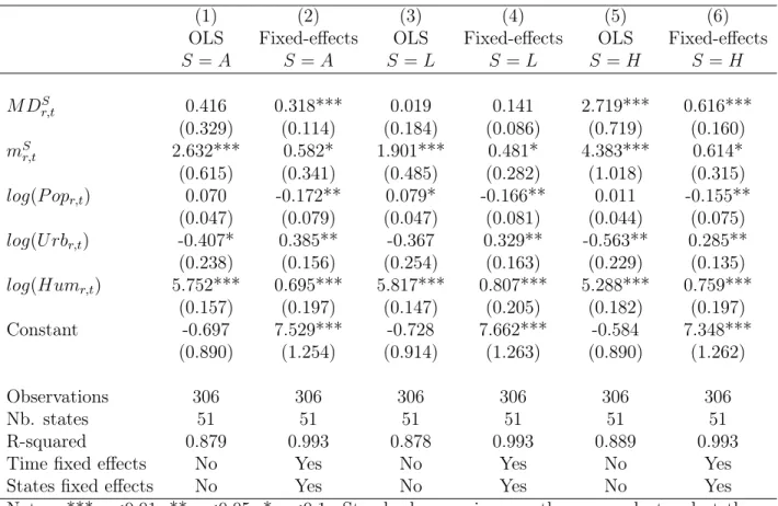
4.1 Pooled OLS and FE Regressions

Table 2 describes the pooled OLS and FE estimates. We produce separate results for the three skill groups, S = (A, L, H), under the same set of control variables, including the

skill-13_{See http://www.infoplease.com/ipa/A0001796.html and http://www.realestate3d.com/gps/}

Table 2: Pooled OLS and FE regressions. Results by skill group (Dep= log(yr,t))

(1) (2) (3) (4) (5) (6)

OLS Fixed-effects OLS Fixed-effects OLS Fixed-effects

S = A S = A S = L S = L S = H S = H M DS r,t 0.416 0.318*** 0.019 0.141 2.719*** 0.616*** (0.329) (0.114) (0.184) (0.086) (0.719) (0.160) mS r,t 2.632*** 0.582* 1.901*** 0.481* 4.383*** 0.614* (0.615) (0.341) (0.485) (0.282) (1.018) (0.315) log(P opr,t) 0.070 -0.172** 0.079* -0.166** 0.011 -0.155** (0.047) (0.079) (0.047) (0.081) (0.044) (0.075) log(U rbr,t) -0.407* 0.385** -0.367 0.329** -0.563** 0.285** (0.238) (0.156) (0.254) (0.163) (0.229) (0.135) log(Humr,t) 5.752*** 0.695*** 5.817*** 0.807*** 5.288*** 0.759*** (0.157) (0.197) (0.147) (0.205) (0.182) (0.197) Constant -0.697 7.529*** -0.728 7.662*** -0.584 7.348*** (0.890) (1.254) (0.914) (1.263) (0.890) (1.262) Observations 306 306 306 306 306 306 Nb. states 51 51 51 51 51 51 R-squared 0.879 0.993 0.878 0.993 0.889 0.993

Time fixed effects No Yes No Yes No Yes

States fixed effects No Yes No Yes No Yes

Notes: *** p<0.01, ** p<0.05, * p<0.1. Standard errors in parentheses are clustered at the state level. The specification is described in Eq. (3). Pooled OLS results are provided in col. 1, 3 and 5; FE results are provided in col. 2, 4 and 6. Results for all immigrants are provided in col. 1 and 2; results for low-skilled immigrants are provided in col. 3 and 4; results for college-educated immigrants are provided in col. 5 and 6. The sample includes the 50 US states and the District of Columbia from 1960 to 2010. The set of control variables includes the immigration rate (mS

r,t), the log of population (log(P opr,t)), the log of urbanization (log(Urbr,t)) and the log of the average educational attainment of the working-age population (log(Humr,t)).

specific immigration rate, mS

r,t, the log of population, log(P opr,t), the log of urbanization, log(U rbr,t), and the log of the average educational attainment of the working-age population, log(Humr,t). In all cases, our standard errors are clustered at the state level in order to correct for heteroskedasticity and serial correlation.

The pooled OLS estimates are reported in col. 1, 3 and 5. We find that the effect of birthplace diversity on GDP per capita is skill specific. Insignificant effects are obtained when diversity is computed using the low-skilled or the total immigrant populations; on the contrary, the association between GDP per capita and birthplace diversity among college-educated immigrants is positive and significant at the 1% level. The coefficient is large,

implying that a 10% increase in high-skilled diversity is associated with a 27.2% increase in GDP per capita.

In columns 2, 4 and 6, we introduce state and year fixed effects in order to mitigate the omitted variable bias. The state fixed effects account for all time-invariant state char-acteristics that could jointly affect productivity and diversity; the year fixed effects account for time-varying sources of change in GDP per capita that are common to all US states. In the FE regressions, the R-squared is above 0.99. The effect of diversity remains highly significant for college-educated immigrants, and remains insignificant for the less educated.14 Interestingly, the inclusion of fixed effects leads to a drop in our estimated diversity coef-ficient. The coefficient of high-skilled diversity is divided by four compared to the pooled OLS regression. This demonstrates that accounting for unobserved heterogeneity is crucial when addressing such an issue. As for our control variables, human capital and urbanization rates are significantly and positively associated with GDP per capita. On the contrary, the correlation between GDP and population size is negative. More interestingly, immigration rates are always positively associated with GDP per capita, and the correlation is always greater for college graduates.

In sum, we find that diversity is positively associated with the level of GDP per capita, but only when diversity is computed on workers performing complex or skill-intensive tasks. On the contrary, diversity among less educated immigrants is neither positively nor negatively correlated with macroeconomic performance. According to our fixed-effect estimates, a 10% increase in high-skilled diversity (i.e. in the probability that two randomly-drawn, college-educated immigrants originate from two different countries of birth) is now associated with a 6.2% increase in GDP per capita. Expressed differently, a one-standard-deviation increase in high-skilled diversity is associated with a 3.2% increase in GDP per capita. This implies that, if all US states had the same level of diversity as the most diverse state in 2010, i.e. the District of Columbia (0.976), the average GDP per capita of the US would be 2.3% larger, the coefficient of variation across states would be 2.4% smaller, and the Theil index would decrease by 3.5%. By comparison, if all US states had the same average level of human capital as the District of Columbia, the average GDP per capita of the US would be 8.3% larger, the coefficient of variation across states would be 9.8% smaller, the Theil index would decrease by 16.1% and the GDP per capita of Hawaii, the least diverse state in 2010 (0.797), would be 11.7% larger. In addition, the US-state average level of diversity among college-educated migrants increased by 7 percentage points between 1960 and 2010; this explains

14_{It is worth noticing that the total diversity index becomes significant at the 1% level when fixed effects}

a 3.5% increase in macroeconomic performance (i.e. only one fiftieth of the total change in the US level of GDP per capita). Although diversity has significant effects on cross-state disparities, its macroeconomic implications are rather limited.

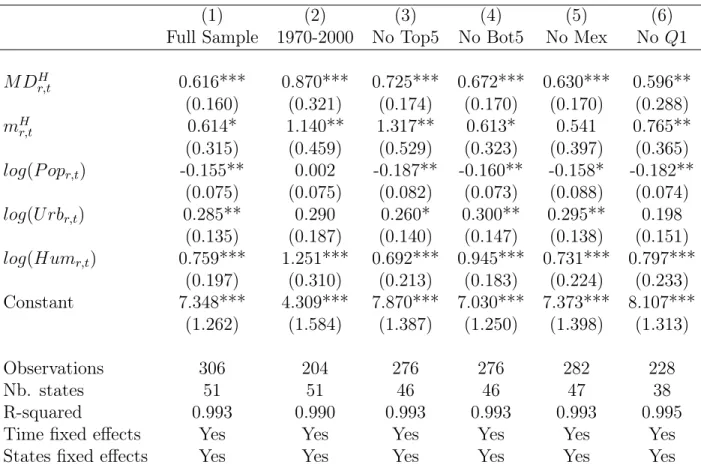
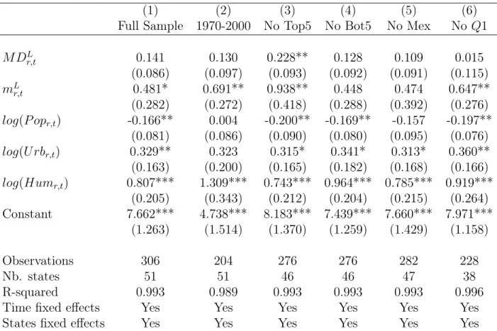
4.2 Robustness by Sub-Sample

In this section, we investigate whether the relationship between diversity and GDP per capita is robust to the exclusion of extreme observations and to the measurement of diversity. Tables 3 and 4 have exactly the same structure, and illustrate the robustness of our FE results by sub-sample. Table 3 reports the results for high-skilled diversity, whereas Table 4 focuses on low-skilled diversity.

In Tables 3 and 4, the benchmark results of Table 2 are reported in col. 1. In col. 2, we limit our sample to the 1970-2000 period, eliminating possible sources of variation prior to the 1965 amendments to the Immigration and Nationality Act, as well as variations driven by the recent evolution of diversity.15 _{Then, in col. 3 and 4, we examine whether the impact} of diversity is driven by the size of the immigrant population; we drop the five US states with the greatest or the smallest immigration rates in 2010, respectively.16 _{In col. 5, we} investigate whether our results are driven by the Mexican diaspora, which represented 30% of the whole immigrant population of the US in 2010. We drop the states located on the US-Mexican border which host 62% of all Mexican immigrants in the US.17 _{Remember that} these states have experienced a drastic decrease in their diversity index (-40% in low-skilled diversity between 1960 and 2010), which is totally due to the rising inflows from Mexico. Finally, in col. 6, we exclude the states in the first quartile (i.e. below Q1) of the 2010 distribution by immigrant population size.

Overall, Tables 3 and 4 show that our FE results are robust to sample selection. In Table 3, the coefficient of high-skilled diversity is always positive, significant, and of the same order of magnitude as the benchmark estimates in col. 1. The positive impact becomes even larger when reducing the time span (0.87) or after excluding the states with the highest immigration rates (0.73). This suggests that high-skilled diversity could generate non-linear effects on macroeconomic performance (e.g. a decreasing marginal impact); we will explore this hypothesis in the next section. As for Table 4, it shows that low-skilled diversity is

15_{Remember that Figure 1(b) shows that the average high-skilled diversity index slightly decreased between}

2000 and 2010

16_{The states with the greatest immigration rates are California, New York, Hawaii, New Jersey, and}

Florida. The states with the smallest rates are West Virginia, Mississippi, Kentucky, South Dakota, and Alabama.

Table 3: Robustness of FE regressions for high-skilled diversity. Alternative sub-samples (Dep= log(yr,t))

(1) (2) (3) (4) (5) (6)

Full Sample 1970-2000 No Top5 No Bot5 No Mex No Q1

M DH_r,t 0.616*** 0.870*** 0.725*** 0.672*** 0.630*** 0.596** (0.160) (0.321) (0.174) (0.170) (0.170) (0.288) mH r,t 0.614* 1.140** 1.317** 0.613* 0.541 0.765** (0.315) (0.459) (0.529) (0.323) (0.397) (0.365) log(P opr,t) -0.155** 0.002 -0.187** -0.160** -0.158* -0.182** (0.075) (0.075) (0.082) (0.073) (0.088) (0.074) log(U rbr,t) 0.285** 0.290 0.260* 0.300** 0.295** 0.198 (0.135) (0.187) (0.140) (0.147) (0.138) (0.151) log(Humr,t) 0.759*** 1.251*** 0.692*** 0.945*** 0.731*** 0.797*** (0.197) (0.310) (0.213) (0.183) (0.224) (0.233) Constant 7.348*** 4.309*** 7.870*** 7.030*** 7.373*** 8.107*** (1.262) (1.584) (1.387) (1.250) (1.398) (1.313) Observations 306 204 276 276 282 228 Nb. states 51 51 46 46 47 38 R-squared 0.993 0.990 0.993 0.993 0.993 0.995

Time fixed effects Yes Yes Yes Yes Yes Yes

States fixed effects Yes Yes Yes Yes Yes Yes

Notes: *** p<0.01, ** p<0.05, * p<0.1. Standard errors in parentheses are clustered at the state level. The specification is described in Eq.(3) and includes all fixed effects. Col. 1 reports the results from Table 2. In col. 2, we exclude observations for the years 1960 and 2010. In col. 3 and 4, we exclude the five US states with the greatest or smallest immigration shares. In col. 5, we exclude US states located on the US-Mexican border. In col. 6, we exclude the lowest quartile in terms of immigrant population. The set of

control variables includes the immigration rate (mS

r,t), the log of population (log(P opr,t)),

the log of urbanization (log(Urbr,t)) and the log of the average educational attainment of

the working-age population (log(Humr,t)).

insignificant in all specifications but one. It only becomes significant in col. 3, when the most diverse states are excluded, but only at the 5% level.

Table 4: Robustness of FE regressions for low-skilled diversity. Alternative sub-samples (Dep= log(yr,t))

(1) (2) (3) (4) (5) (6)

Full Sample 1970-2000 No Top5 No Bot5 No Mex No Q1

M DL_r,t 0.141 0.130 0.228** 0.128 0.109 0.015 (0.086) (0.097) (0.093) (0.092) (0.091) (0.115) mL r,t 0.481* 0.691** 0.938** 0.448 0.474 0.647** (0.282) (0.272) (0.418) (0.288) (0.392) (0.276) log(P opr,t) -0.166** 0.004 -0.200** -0.169** -0.157 -0.197** (0.081) (0.086) (0.090) (0.080) (0.095) (0.076) log(U rbr,t) 0.329** 0.323 0.315* 0.341* 0.313* 0.360** (0.163) (0.200) (0.165) (0.182) (0.168) (0.166) log(Humr,t) 0.807*** 1.309*** 0.743*** 0.964*** 0.785*** 0.919*** (0.205) (0.343) (0.212) (0.204) (0.215) (0.264) Constant 7.662*** 4.738*** 8.183*** 7.439*** 7.660*** 7.971*** (1.263) (1.514) (1.370) (1.259) (1.429) (1.158) Observations 306 204 276 276 282 228 Nb. states 51 51 46 46 47 38 R-squared 0.993 0.989 0.993 0.993 0.993 0.996

Time fixed effects Yes Yes Yes Yes Yes Yes

States fixed effects Yes Yes Yes Yes Yes Yes

Notes: *** p<0.01, ** p<0.05, * p<0.1. Standard errors in parentheses are clustered at the state level. The specification is described in Eq.(3) and includes all fixed effects. Col. 1 reports the results from Table 2. In col. 2, we exclude observations for the years 1960 and 2010. In col. 3 and 4, we exclude the five US states with the greatest or smallest immigration shares. In col. 5, we exclude US states located on the US-Mexican border. In col. 6, we exclude the lowest quartile in terms of immigration rate. The set of control

variables includes the immigration rate (mS

r,t), the log of population (log(P opr,t)), the

log of urbanization (log(Urbr,t)) and the log of the average educational attainment of the

working-age population (log(Humr,t)).

4.3 Alternative Measures of Diversity

This subsection investigates the robustness of our results to the measurement of diversity. Figure 3 and Table 5 report the results obtained for alternative diversity indices, accounting for the age of entry and for the legal status of immigrants.

The diversity indices used in our benchmark regressions are computed for the total popula-tion of working-age immigrants, whatever their age of entry in the US. As birthplace diversity conceivably reflects complementarities between individuals trained in different countries, it

can be argued that immigrants who arrived in the US at different ages generate different levels of complementarity in skills and ideas with the native workforce. However, the role of the age of entry is unclear. On the one hand, immigrants with a longer foreign education are likely to bring more complementarities. On the other hand, immigrants who were partly educated in the US may have more transferable skills and a greater potential to interact with natives. To investigate this issue, we compute the diversity index using various samples of immigrants, and we include these alternative indices in Eq. (3). More precisely, we exclude from the immigrant population the individuals who arrived in the US before a given age threshold, which ranges from 5 to 25 in one-year intervals.

For each skill group, Figure 3 reports the marginal effect of diversity and its confidence interval as a function of the age-of-entry threshold.18 _{As information on age of entry is} not available in the 1960 census, our sample covers the 1970-2010 period. For this time span, the coefficients of the benchmark FE regressions (without controlling for age of entry) are equal to 0.835 for high-skilled diversity (significant at the 1% level), and to 0.088 for skilled diversity (insignificant). Whatever the age-of-entry threshold, the effect of low-skilled diversity is insignificant. Nevertheless, the age of entry matters for college graduates. Although the coefficient of high-skilled diversity is always positive and significant, the largest effects are obtained when the immigrant population includes individuals who arrived before age 20. Alesina et al. (2016) consider three age thresholds (12, 18, and 22). They show that the positive effect of birthplace diversity slightly decreases when eliminating children immigrants, but always remains large and significant. Conversely, our results suggest that the greatest levels of complementarity are obtained when immigrants acquired part of their secondary education abroad and their college education in the US.

We now investigate the role of undocumented migration in governing the skill-specific effects of diversity. The US census counts every person regardless of immigration status. Hence, undocumented immigrants influence our diversity index. This can be a source of concern as undocumented migrants are likely to be less educated than the legal ones and to contribute differently to GDP, either because their productive activities are not recorded in the official GDP or because they are employed in jobs/sectors where skill complementarities are smaller. This could explain why the effect of low-skilled diversity is insignificant in most of our regressions. To explore this hypothesis, we follow on the “residual methodology” proposed by Borjas (2016) to identify the number of legal and undocumented immigrants by skill group. It consists in using individual characteristics to proxy the legal status of

Figure 3: Marginal effect of MDS

r,t on log(yr,t) Results for different age-of-entry thresholds (1970-2010)

(a) High-skilled

(b) Low-skilled

Source: Authors’ elaboration on IPUMS data. Notes: The two graphs report the marginal effect of MDS

r,t

on log(yr,t) when the immigrant population is restricted to individuals who arrived in the US after age

X. Marginal effects are obtained using our main specification Eq. (3) which includes state and year fixed

effects, as well as the immigration rate (mS

r,t), the log of population (log(P opr,t)), the log of urbanization

US immigrants. In this work, we use five characteristics (citizenship, employment industry, occupation, whether the individual receives any assistance, and the spouse’s legal status ) and, due to data availability, we apply the residual methodology to the census years 1980 to 2010. We obtain similar results as in Borjas (2016). For the year 2010, our estimated proportions of undocumented immigrants are equal to 23% in California, 7% in New York, and 15% in Texas; for the same states in the year 2012, Borjas (2016) also obtains 23%, 7%, and 15%. Moreover, the observable characteristics of our undocumented population are also similar. We identify 50% of males and 36% of college graduates; Borjas (2016) obtains 55% and 40%, respectively.

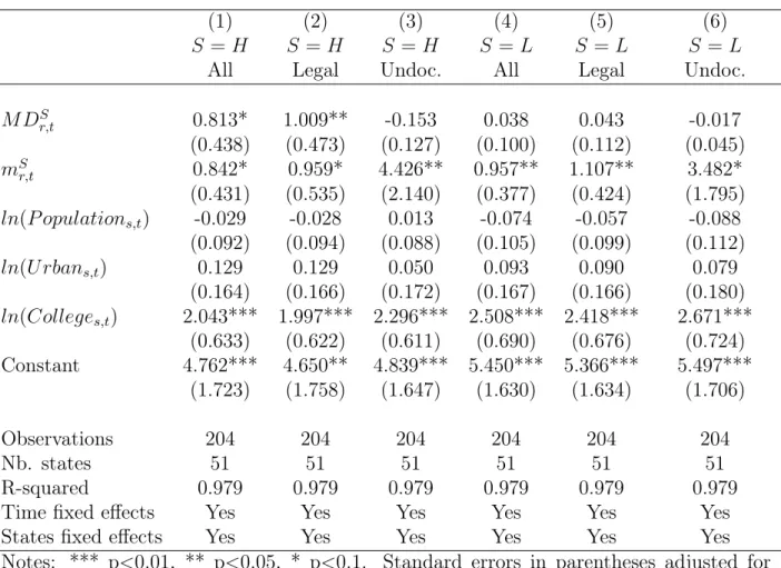
As a robustness check, we thus compute the diversity indices on the legal and undocu-mented immigrant populations, and include them separately in our FE regressions. Table 5 shows the results for the two skill groups. Col. 1 and 4 give the results of the benchmark specification for the 1980-2010 period. We still observe a positive and significant effect of high-skilled diversity (although the significance of the coefficient is smaller over this period) and an insignificant effect of low-skilled diversity. As far as high-skilled immigrants are con-cerned, distinguishing between legal and undocumented immigrants yields different effects (see col. 2 and 3). Diversity among undocumented immigrants has no significant effect, while diversity among legal immigrants has a positive and significant effect at the five percent level. On the contrary, controlling for the legal status of low-skilled immigrants does not modify our conclusions. Col. 5 and 6 confirm that the insignificant effect of low-skilled diversity cannot be attributed to the greater proportion of undocumented migrants in this group (on average, 17% for the US in 2010).

Table 5: Robustness of FE regressions.

Results by legal status and skill group (Dep= log(yr,t))

(1) (2) (3) (4) (5) (6)

S = H S = H S = H S = L S = L S = L

All Legal Undoc. All Legal Undoc.

M DS r,t 0.813* 1.009** -0.153 0.038 0.043 -0.017 (0.438) (0.473) (0.127) (0.100) (0.112) (0.045) mS r,t 0.842* 0.959* 4.426** 0.957** 1.107** 3.482* (0.431) (0.535) (2.140) (0.377) (0.424) (1.795) ln(P opulations,t) -0.029 -0.028 0.013 -0.074 -0.057 -0.088 (0.092) (0.094) (0.088) (0.105) (0.099) (0.112) ln(U rbans,t) 0.129 0.129 0.050 0.093 0.090 0.079 (0.164) (0.166) (0.172) (0.167) (0.166) (0.180) ln(Colleges,t) 2.043*** 1.997*** 2.296*** 2.508*** 2.418*** 2.671*** (0.633) (0.622) (0.611) (0.690) (0.676) (0.724) Constant 4.762*** 4.650** 4.839*** 5.450*** 5.366*** 5.497*** (1.723) (1.758) (1.647) (1.630) (1.634) (1.706) Observations 204 204 204 204 204 204 Nb. states 51 51 51 51 51 51 R-squared 0.979 0.979 0.979 0.979 0.979 0.979

Time fixed effects Yes Yes Yes Yes Yes Yes

States fixed effects Yes Yes Yes Yes Yes Yes

Notes: *** p<0.01, ** p<0.05, * p<0.1. Standard errors in parentheses adjusted for clustering at the state level. Col. 1 and 4 report the coefficient of the benchmark sample over the 1980-2010 period and for high-skilled and low-skilled immigrants, respectively. In col. 2 and 5, the diversity indices are computed for the legal immigrant population only. In col. 3 and 6, we use the undocumented immigrant population only.

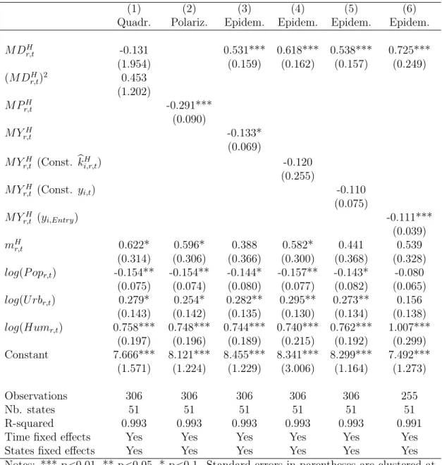
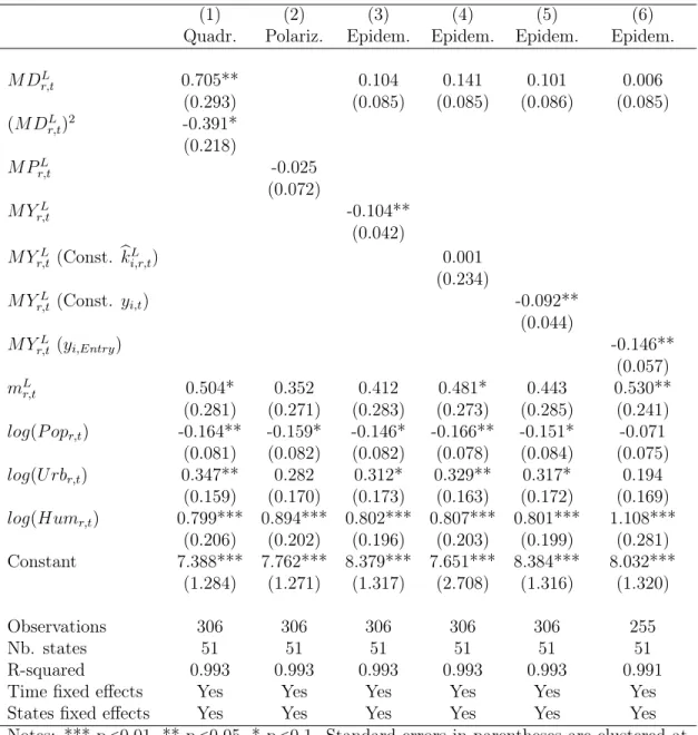
4.4 Alternative Specifications

In Tables 6 and 7, we report the results obtained under three alternative specifications de-tailed in Section 3.2. First, we consider a quadratic specification a la Ashraf and Galor (2013), and supplement the benchmark model in Eq. (3) with the squared index of birth-place diversity. If an optimal level of diversity exists, we should find a positive coefficient for the linear term, and a negative coefficient for the squared term. The results for high-skilled and low-skilled diversity are presented in col. 1 of the two different tables, respectively. Sec-ond, we replace the diversity index by a polarization index a la Montalvo and Reynal-Querol (2003); the latter is denoted by (MP_{r,t) and is computed for the immigrant population only.}S