Avoiding Routing Loops in a Multi-Stack WSN

HAL Id: hal-01790284

https://hal.archives-ouvertes.fr/hal-01790284

Submitted on 11 May 2018

HAL is a multi-disciplinary open access

archive for the deposit and dissemination of

sci-entific research documents, whether they are

pub-lished or not. The documents may come from

teaching and research institutions in France or

abroad, or from public or private research centers.

L’archive ouverte pluridisciplinaire HAL, est

destinée au dépôt et à la diffusion de documents

scientifiques de niveau recherche, publiés ou non,

émanant des établissements d’enseignement et de

recherche français ou étrangers, des laboratoires

publics ou privés.

Avoiding Routing Loops in a Multi-Stack WSN

Nancy Rachkidy, Alexandre Guitton, Michel Misson

To cite this version:

Nancy Rachkidy, Alexandre Guitton, Michel Misson. Avoiding Routing Loops in a Multi-Stack WSN.

Journal of Communications, Academy Publisher, 2013, �10.12720/jcm.7.2.89-105�. �hal-01790284�

Avoiding Routing Loops in a Multi-Stack WSN

Nancy El Rachkidy

, Alexandre Guitton

, Michel Misson

(1) Clermont Universit´e, Universit´e Blaise Pascal, LIMOS, BP 10448, F-63000 Clermont-Ferrand, France (2) Clermont Universit´e, Universit´e d’Auvergne, LIMOS, BP 10448, F-63000 Clermont-Ferrand, France

(3) CNRS, UMR 6158, LIMOS, F-63173 Aubi`ere, France Emails:{nancy,guitton,misson}@sancy.univ-bpclermont.fr

Abstract—Wireless sensor networks are envisioned to

support an increasing number of applications having various quality of service (QoS) requirements. A possibility to provide a large variety of QoS is to deal with multi-stack WSN where several routing and MAC protocols coexist in the same network. However, routing loops can occur when several routing protocols are used alternatively. Such loops can yield to large delays and high packet loss, and should therefore be avoided. In this paper, we propose a three-step solution to solve the loop problem. The first step describes a sufficient condition to determine when two arbitrary routing protocols can be used without producing loops. The second step states that loops can be avoided if some nodes refrain temporarily from sending a packet. The third step proposes a mechanism that guarantees that no loops are produced for any pair of routing protocols. Our solution is proved through theoretical analysis, and its performance is evaluated through extensive simulations. It requires a limited energy overhead and limited computation capabilities for the network devices.

Index Terms—Routing protocols, multi-purpose wireless

sensor networks, routing loops.

I. INTRODUCTION

Wireless sensor networks (WSNs) are increasingly used in order to monitor the environment or to detect critical events. A WSN is often designed to meet the require-ments of a specific application. However, this approach is showing its limits when the traffic types generated by the application has very different profiles (e.g., periodic traffic, daily log transfer, alarm events), or when the number of application increases. A recent trend is to deploy a general-purpose WSN that is used by several applications simultaneously [1].

Existing WSNs are traditionally operated using a single routing protocol and a single MAC protocol. However, this pair of protocols cannot provide the best network performance for all QoS [2], [3]. Indeed, a given pair is designed for a specific type of traffic: some protocols might provide a high reactivity to alarm events, while others might be able to extend the network lifetime. Another issue with application-specific WSNs is that each application has to support the full cost of deployment. Some researchers have proposed multi-purpose WSNs,

Manuscript received November 30, 2012; accepted February 17, 2013. Corresponding author email: guitton@sancy.univ-bpclermont.fr. doi:10.12720/jcm.7.2.89-105 (doi:10.43.04/jcm.v.n.p-p)

where a single deployment can serve several applica-tions [4], [5]. Although using several protocols in a mote increases the code size, a modular approach can reduce the code size by merging redundant code [6].

A way to provide several QoS is to have two (or possi-bly more) pairs of MAC and routing protocols operating in the same WSN. For instance, such a mechanism is used in the following protocols:

• In the IEEE 802.15.4 standard [7], where a slotted

carrier-sense multiple access algorithm (CSMA) with collision avoidance is used during the contention access period, and a direct access algorithm is used during the contention-free period.

• In Z-MAC [8], where a CSMA protocol is used

in low traffic conditions and a time-division-based MAC protocol is used in high traffic conditions.

• In Funneling MAC [9], where an hybrid CSMA and

time-division MAC protocol is used in the congested region near the sink, and a pure CSMA protocol is used far away from the sink.

• In MaCARI [10] where a time-division-based MAC

protocol with a hierarchical routing is used during a time period, and a collision-based MAC protocol with EOLSR [11] is used during another.

Multi-stack architectures can be implemented by scheduling the activity of all the nodes in the network, and by ensuring that at any given time, only one pair of routing and MAC protocols is active for all the nodes. More specifically, time is divided into periods and during each period pi, a routing protocolRiand a MAC protocol

Miare activated, as shown on Figure 1. It can be noticed

that a synchronization mechanism precedes the first pe-riod: it ensures that all the nodes of the network have a common time reference, and also informs nodes about the length of each period pi. The multi-stack architecture

approach was formalized in [12].

00 00 11 11 00 00 11 11 000 000 111 111[R1, M1] [R1, M1] [R2, M2] [R2, M2] schedule synchronization time

Figure 1. In this schedule shared by all the nodes, the pairs[R1, M1] and[R2, M2] are activated sequentially and periodically.

Scheduling several pairs of routing and MAC protocols leads to two main issues. The first issue comes from the

fact that packets have to be marked at the application layer so that they can be dispatched to the correct routing protocol. A packet marked with i can only be sent during period pi. This ensures that all the nodes apply the same

routing protocol to the same packet, and thus ensures that consistent routing decisions are taken. If the current period is not pi, a packet marked with i has to wait

for the next pi to be sent, which increases the delay.

The second issue is the dimensioning of the periods. A static dimensioning is not suitable for bursty traffic. If the period is too short for the traffic, some packets have to wait for the next occurrence of the period to be sent. If the period is too large for the traffic, time is wasted. A dynamic dimensioning requires complex algorithms and a significant control overhead in order to adapt the periods to the traffic generation.

In this paper, we study a multi-stack architecture where packet exchange is allowed between the pairs of routing and MAC protocols. We focus on the occurrence of loops in the network, which are caused solely by the routing protocols. More specifically, we study when and how to allow packets to be routed by different routing protocols. In other words, our approach can be used to route packets marked with i according toRj (with i6= j),

without causing the packets to enter a routing loop. Our approach reduces the impact of the two issues mentioned previously, as packets can now be sent during several periods.

The remainder of this paper is organized as follows. Section II describes briefly the routing protocols we used as examples in our simulations. Section III highlights the risks of having loops when using several routing protocols to route the same packet. Section IV describes our three-step solution to avoid loops. The first three-step shows when routing protocols are compatible, which means that they cannot produce loops. The second step describes how to design a holding function, which is used by nodes to refrain from sending packets when these packets might enter a loop. The third step describes how to apply a generic holding function to any arbitrary schedule. Each step is proved theoretically. In Section V, we make extensive simulations to quantify the routing loop and the benefits of our approach. Finally, in Section VI, we give conclusions and perspectives.

II. STATE OF THEART

This section briefly describes some routing protocols and divides them into two categories: the routing proto-cols that might generate loops, and the loop-free routing protocols. In the remainder of this work, we focus on routing protocols that do not yield to routing loops by themselves.

A. Routing Protocols Generating Loops

The main task of a routing protocol is to forward a packet to a given destination, without generating too much overhead or routing loops. Some protocols, how-ever, might cause routing loops in some conditions. The

collection tree protocol (CTP) [13] is an example of such protocols.

CTP is a tree-based collection protocol. Some nodes in the network advertise themselves as tree roots, and nodes form a set of routing trees from these roots using an additive metric based on the expected number of transmissions. This metric assumes that nodes use link-level retransmissions. Given a choice of valid routes, CTP chooses the one with the lowest number of expected transmissions.

Routing loops can appear in a CTP network, when a node chooses a new route that has a significantly higher cost than the previous one. To reduce this problem, a specific frame is broadcasted when such a new route is chosen. Also, if some nodes are disconnected from the network, the cost for the unreachable nodes increases to infinity. That is why CTP assumes that a node is unreachable when the value exceeds a given threshold.

B. Loop-Free Routing Protocols

In this part, we describe the behavior of routing pro-tocols that do not yield to routing loops by themselves. We use these examples of routing protocols later in the paper.

1) Hierarchical Tree Routing Protocol: The hierarchi-cal tree routing protocol of ZigBee [14] is referred to as the tree protocol in the following of this paper. Using this protocol, communications follow the links of a tree. When a router at depth d receives a packet, the router checks whether the destination is within its own address space or not. If it is the case, the destination is a descendant of the router: the router computes for which child the packet has to be sent. Otherwise, the router sends the packet to its parent.

The tree protocol allows high energy savings [15]. Indeed, the routing decision can be made without ex-changing routing tables between routers. Thus, the control overhead is limited to the tree maintenance. Moreover, the energy overhead is limited: when a router r is active, only its parent and children have to be active, while the other potential neighbors can be inactive. However, the tree protocol produces non-optimal routes in terms of hop-count.

2) Shortcut Tree Routing Protocol: The shortcut tree routing protocol [16], referred to as the shortcut protocol in the following, enhances the tree protocol by using the knowledge of one-hop neighbors. To route a packet using the shortcut protocol, a router r forwards it to the neighbor providing the smallest expected number of hops according to the distance on the tree.

The shortcut protocol is able to reach the destination by using less hops than the tree protocol. However, all the neighbors of a router have to be active when the router has to transmit a packet, as they are potential next hops, which increases the energy consumption.

3) Shortest Path Routing Protocols: Shortest path rout-ing protocols are based on optimal paths in terms of number of hops. They are usually not energy efficient: an

high control overhead is required in order to determine the optimal path. Moreover, all the neighbors of a router have to be active when the router sends a frame, which consumes energy. Such protocols include AODV [17] and OLSR [18]. In this work, we use OLSR as an example of shortest path routing protocol.

Optimized Link-State Routing (OLSR) protocol [18] is a routing protocol designed for mobile ad-hoc networks. It is a link-state routing protocol, based on the concept of multipoint relays (MPRs). MPRs form a subset of one-hop neighbors of a node r that are in range of all two-hop neighbors of r. When r has to send a packet, it sends it to one of its MPR, which can in turn forward the packet to the correct destination. Instead of requiring all the neighbors of r to be active when r transmits a packet, only the MPRs of r have to be active.

III. PROBLEM: LOOPOCCURRENCE

The problem of operating several routing protocols alternatively is that routing loops might occur in the network, when different routing protocols are involved to forward the same packets. Subsection III-A gives technical details about multi-stack architectures, which can support several routing protocols. Subsection III-B shows why and how several routing protocols can be used in order to forward the same packet. Subsection III-C describes the problem of loop occurrence through an example.

A. How to Make Several Pairs of Routing and MAC Protocols Coexist?

Multi-stack architectures help providing several QoS for the applications. The routing and MAC protocols used in such architectures can be activated alternatively, according to a schedule similar to the one shown on Figure 1. In the basic model, applications mark packets with a number i, which corresponds to the routing and MAC protocols (Ri,Mi) they require. Each routing

protocolRi adds the packets in a queueQi. A common

MAC layer determines what is the current time period pi, deduces which MAC protocol Mi is active, extracts

a packet from the corresponding queueQi, and sends the

packet. The process is similar for the reception. A packet marked at the source with i is forwarded during period pi

by all the nodes, and is always processed using the same Ri, which guarantees that no routing loop occurs1.

This architecture has two main drawbacks. First, a packet marked with i cannot be sent during a period pj,

with i 6= j. Thus, packets have to wait for the suitable period in order to be transmitted, which increases the delay. Second, the dimensioning and adaptation of the duration of each period pi to the traffic requires a high

overhead, especially when the traffic production is bursty.

1_{Provided that R}

iis loop-free.

B. Queue-Exchange Mechanism

In [19], we allowed the exchange of packets from one queue to another. When a MAC protocolMi has sent all

the packets stored in its queue Qi, Mi can extract the

packets from another queueQj (with i6= j) in order to

use the remaining time of period pi. However, in this case,

the next hop computed according toRj can be inactive

in period pi. Thus, the next hop of packet marked with j

has to be recomputed according toRi and sent according

toMi.

This queue-exchange mechanism can solve the two main drawbacks of multi-stack architectures. First, pack-ets do not need to wait for a specific period pi: they can be

processed and sent during any period. Second, an accurate dimensioning of the schedule is not crucial anymore: if a period is too short for the packets dedicated to it, another routing protocol can forward the additional packets, and if a period is too large, time is not wasted since this period can be used to send packets dedicated to other periods.

C. Example of Loop Occurrence

When a packet can be forwarded according to several routing protocols, routing loops can occur. In this paper, we focus on removing these loops, rather than on simply observing their impact on the network performance (as was done in [19]).

In the following, we focus on the routing protocols, since they are the only cause of routing loops in the network. We consider that a routing loop is generated in the network when a node forwards the same packet more than once.

Figure 2 depicts an example where a packet enters a routing loop because of the use of two different routing protocols. We assume that node A has a packet to send to node E,R1 (represented using solid arrows) and R2

(represented using dashed arrows) alternate every two hops. Our scenario starts at the beginning of period p1.

A sends the packet to B, which sends it to D. Then the period changes to p2, and thus the routing protocol

changes to R2. D sends the packet to B, which sends

it to C. Then, R1 is reactivated. C sends the packet to

D, which sends it to E. The path followed by the packet is(A, B, D, B, C, D, E), which corresponds to six hops. Using the multi-stack architecture with queue exchange increases the distance to the destination, because of a routing loop. A B C D E

Figure 2. A routing loop occurs when A sends a packet to E, if the protocols alternate every two hops and if the first protocol used is the one with solid lines.

IV. SOLUTION: THREE-STEPAPPROACH TOAVOID ROUTINGLOOPS

The main purpose of this paper is to propose a solution to routing loops, which occur when packet exchanges are allowed in a multi-stack architecture.

In this section, we describe our three-step approach. First, we study compatible routing protocols, i.e. protocols that can coexist without producing loops. Second, we in-troduce delayable routing protocols, which use a holding function in order to become compatible. However, this holding function might be difficult to compute for arbi-trary protocols. Third, we propose a combined solution providing a simple holding function for any schedule of arbitrary protocols.

A. Step 1: Compatible Routing Protocols

LetR be a routing protocol, and V be a set of nodes. For each destination d∈ V and for any node n ∈ V \{d}, the next hop of n for destination d by R is denoted by R(n, d). We consider that R(d, d) is not defined.

Let R1 and R2 be two routing protocols. We define

by routing loop the fact that a node forwards the same packet more than once.

Definition 1 (Compatible routing protocols). Two routing

protocols R1 and R2 are compatible if any node can decide arbitrarily to forward a packet according to R1 or to R2, without generating a loop, in order to reach the destination.

Theorem 1. LetR1 andR2 be two routing protocols, V be a set of nodes and d∈ V a destination. If there exists

a function fd : V \{d} → IN such that ∀n ∈ V \{d}, max{fd(R1(n, d)), fd(R2(n, d))} < fd(n), then R1and

R2 are compatible.

Proof: Let d ∈ V be a destination. We consider that there exists a function fd that satisfies the property

fd(d) = 0 and ∀n ∈ V \{d}, max{fd(R1(n, d)), fd(R2

(n, d))} < fd(n). We aim to show that every path starting

from an arbitrary node n reaches d in a finite number of hops without generating routing loops. In other words, we aim to show that for every sequence (ri) of routing

decisions (with ri ∈ {1, 2} for every i), if (ri) is long

enough to reach d (possibly infinite if d can never be reached), the unique path starting from n and following the routing decisions(ri) reaches d in a finite number of

hops without generating routing loops.

Let (ri) be a sequence of routing decisions. Let us

define the path according to(ri) by p = (n0, n1, n2, . . .),

with n0= n and ni+1= Rri(ni, d) for every node ni∈ V\{d}. By construction, p is unique (as (ri) is fixed).

First, let us show that: (1) if p is infinite, all the nodes of p belong to V\{d}, (2) if p is finite, all the nodes of p, except the last one, belong to V\{d}.

If p is infinite, at every node ni of p corresponds a node

ni+1 in p, which is possible only if ni ∈ V \{d}. Thus,

all the nodes of p are in V\{d}. If p is finite, it can be written as(n0, n1, n2, . . . , nk). By construction, for every

i∈ [0; k − 1], ni+1 exists, which means that ni∈ V \{d}.

nk does not belong to V\{d} as nk+1 is not defined

(notice that the sequence(ri) is chosen long enough).

Now, let us show that p is finite. Let us proceed by con-tradiction by supposing that p is infinite. As p is infinite, all the nodes of p are in V\{d}. Using p, we can build the infinite sequence s = (fd(n0), fd(n1), fd(n2), . . .)

by applying the function fd at each node of p. Notice

that for each node ni ∈ V \{d}, we have fd(ni+1) =

fd(Rri(ni, d)) < fd(ni) by definition of fd. The se-quence s is thus strictly decreasing. However, s is defined in IN . It is not possible to have an infinite sequence strictly decreasing in IN : the assumption that p is infinite is false, therefore p is a finite sequence.

As we have shown that p is finite, let us show that p reaches d. As p is finite, all the nodes of p, except the last one nk, belong to V\{d}. The node nk is defined as

nk ∈ V and nk does not belong to V\{d}, nk is then

equal to d. In other words, if nk belongs to V\{d}, nk+1

would exist in p, and nk would not be the last node in p.

Now, as we know that p is finite and that p reaches d, let us show that p is free of routing loop. By contradiction, we suppose that p passes twice by the same node. There exists thus x and y such that nx =

ny, with x < y. Let us build the sequence s =

(fd(n0), fd(n1), fd(n2), . . . , fd(nx), . . . , fd(ny)). Let us

consider two cases:

• y is equal to k. This means that ny = nk. Since nx=

ny and nk = d, nx = d. We have a contradiction

because nx+1 exists in p (as there exists ny with

y > x) but is not defined because nx= d.

• y is not equal to k. Thus, ny is not the last

node in p. Consequently, all the nodes of p from n0 to ny belong to V\{d}. So, for every ni ∈

(n0, n1, n2, . . . , nx, . . . , ny), we have fd(ni+1) =

fd(Rri(ni, d)) < fd(ni). The sequence s is thus strictly decreasing which requires that fd(nx) <

fd(ny) as x < y. However, as nx = ny, we have

fd(nx) = fd(ny). We have a contradiction.

In both cases, we have a contradiction. Considering that p passes twice by a same node is thus not valid.

We have shown that the unique path p reaches d with a finite number of hops, without generating any routing loop.R1 andR2 are thus compatible.

More intuitively, the function fdcould be defined as the

distance to the destination. For any routing protocolR1

orR2, the next hop ni+1 corresponds to a value fd(ni+1)

lower than the value fd(ni) of node ni: in all cases, the

path p converges to the destination. For all the nodes, except the destination d, there always exists a next hop according toR1 andR2: the construction of the path is

stopped only when d is reached. The path convergence to d results from the necessary decreasing of the value of fd

in each node (except in d).

In order to prove that two routing protocols are com-patible, the difficulty lies in finding the function fd.

Property 1. The tree protocol and the shortcut protocol

Proof: Let us consider that R1 is the tree protocol

andR2is the shortcut protocol. Let us build fdas follows:

for each node n ∈ V , fd(n) is the number of hops

remaining on the tree in order to reach d.

Let us show that fd satisfies the conditions of

Theo-rem 1. First of all, fdis a function defined from V to IN

and fd(d) = 0. For all nodes n ∈ V \{d}:

• fd(n) > 0 because n 6= d and fd is a distance. • fd(n) > fd(R1(n, d)). Indeed, as R1 is the tree

protocol and fd is the distance on the tree, the

next hop of n according to R1 is one hop closer

to the destination than n. Thus, we have fd(n) =

fd(R1(n, d)) + 1.

• fd(n) > fd(R2(n, d)). Indeed, R2 is the shortcut

protocol. Let x= R2(n, d). x is the node among the

neighbors of n that minimizes the remaining distance to d, i.e. for every neighbor v of n, fd(v) ≥ fd(x).

However, the next hop of n on the tree,R1(n, d) is a

neighbor of n. We have thus fd(R1(n, d)) ≥ fd(x).

Noticing that fd(n) > fd(R1(n, d)) (as shown

above) and that fd(x) = R2(n, d), we have fd(n) >

fd(R2(n, d)).

Thus, fd(n) > max{fd(R1(n, d)), fd(R2(n, d))}.

Property 2. Any two shortest path routing protocols are

compatible.

Proof:This property can be proved by computing fd

as follows: for each node n ∈ V , fd(n) is the smallest

number of hops to reach the destination d.

B. Step 2: Delayable Routing Protocols

Some pairs of routing protocols are not compatible. For instance, the tree protocol (respectively, the shortcut protocol) is not compatible with a shortest path routing protocol (as shown later in Figure 3).

When two routing protocols are not compatible, a node can decide to hold a packet temporarily rather than to risk sending it into a routing loop. The forwarding of such a packet is delayed until the other protocol routes the packet.

Definition 2 (Delayable routing protocols). Two routing

protocols R1 and R2 are delayable using a holding function hd if every packet for destination d reaches d without generating a routing loop and without being held by a node for an infinite time. Packets are held based on the following computation:

• if hd(n) ≤ hd(Rri(n, d)), node n holds the packet,

• otherwise, node n forwards the packet according to

Rri, where ri∈ {1, 2} is computed locally by n.

Theorem 2. Let R1 and R2 be two routing protocols that alternate in finite time, V be a set of nodes and

d ∈ V a destination. If there exists a function hd :

V → IN such that hd(d) = 0 and ∀n ∈ V \{d},

hd(n) > min{hd(R1(n, d)), hd(R2 (n, d))}, and if the routing protocols alternate after a finite time, then R1 andR2 are delayable using function hd.

Proof: Notice that this proof is similar to the proof of Theorem 1, but takes into account the fact that a node can hold a packet.

Let d ∈ V be a destination. Let us suppose that there exists a function hd satisfying the property hd(d) = 0

and ∀n ∈ V \{d}, hd(n) > min{hd(R1(n, d)), hd

(R2(n, d))}. We aim to show that every path starting

from an arbitrary node n reaches d in a finite number of hops, without generating routing loops (holding a packet in a node is not considered as a routing loop). In other words, we aim to show that for every sequence of routing decisions (ri) (with ri ∈ {1, 2} for every i), if (ri) is

long enough and does not contain an infinite sequence of consecutive identical values (as the protocols alternate after a finite time), then the unique path starting from n and following the routing decisions (ri) reaches d in a

finite number of hops, without generating a routing loop. Let us consider that (ri) is a sequence of routing

decisions that is long enough, and which does not contain an infinite sequence of consecutive identical values. We define the path following the routing decisions (ri) by

p= (n0, n1, n2, . . .), with n0 = n and for every node

n∈ V \{d}:

• if hd(n) ≤ hd(Rri(n, d)), then ni holds the packet, and thus ni+1 = ni (which is not a routing loop). • otherwise, ni+1= Rri(ni, d).

By construction, p is unique (as(ri) is fixed).

Let us show first that:

• if p is infinite, all the nodes of p belong to V\{d}, • if p is finite, all the nodes of p, except the last one,

belong to V\{d}.

If p is infinite, to every node niof p corresponds another

node ni+1 in p, which is possible only if ni ∈ V \{d}.

Thus, all the nodes of p belong to V\{d}. If p is finite, we can write it as(n0, n1, n2, . . . , nk). By construction,

for every i∈ [0; k − 1], ni+1does exist, which means that

ni∈ V \{d}. nkdoes not belong to V\{d} because nk+1

is not defined (notice that the sequence(ri) was chosen

long enough).

Now, let us show that p is finite. By contradiction, we suppose that p is infinite. As p is infinite, p is built from nodes that belong to V\{d}. We can build the infinite sequence s= (hd(n0), hd(n1), hd(n2), . . .) by applying

hd at each node of p. Note that for each ni of p, as ni

belongs to V\{d}, we have hd(ni+1) ≤ hd(ni), because: • if hd(ni) ≤ hd(Rri(ni, d)), the packet is held, thus

ni+1= ni and hd(ni+1) = hd(ni).

• otherwise, we have hd(ni) > hd(Rri(ni, d)), which means that hd(ni+1) = hd(Rri(ni, d)) < hd(ni). The sequence s is thus decreasing (although not strictly). However, it only keeps the same value when the packet is held by a node. We aim to show now that s does not remain constant for an infinite time, which means that if ni decides to hold the packet, there exists a

j = i + α, with α > 0 and α finite, such that hd(nj) > hd(Rrj(nj, d)). As the protocols alternate in finite time,(ri) does not contain an infinite sequence of

consecutive identical values. Let us choose the smallest j= i+α, with α > 0 and α finite, such that rj6= ri. As j

is the smallest valid integer, ni= ni+1= . . . = nj. As ni

has decided to hold the packet, hd(ni) ≤ hd(Rri(ni, d)). As ni = nj, we have hd(nj) ≤ hd(Rri(nj, d)). As rj6= ri, we have{ri, rj} = {1, 2}. Furthermore, we have

hd(nj) > min{hd(R1(nj, d)), hd(R2(nj, d))} by

defini-tion of hd, which means that hd(nj) > hd(R1(nj, d)) or

hd(nj) > hd(R2(nj, d)) (notice that 1 and 2 have been

replaced by i and j). In other words, we can say that hd(nj) > hd(Rri(nj, d)) or hd(nj) > hd(Rrj(nj, d)). It is the second hypothesis that is true, because we said that hd(nj) ≤ hd(Rri(nj, d)). The sequence s is thus decreasing but does not remain constant for an infinite time. However, s takes its values in IN . It is not possible to have an infinite sequence decreasing, constant only for a finite time, and having its values in IN : the hypothesis of having p infinite is thus wrong, and p is a finite sequence. Now that p is shown to be finite, let us show that p reaches d. As p is finite, all the nodes of p, except the last one nk, belong to V\{d}. nk is such that nk ∈ V

and nk does not belong to V\{d}. nk is thus equal to d.

Now, as we know that p is finite, and that p reaches d, let us show that p is free of routing loop. First, note that if there exists x such that nx = nx+1 in

p, the packet has been held by nx. By contradiction,

let us suppose that the packet was not held by nx.

We have thus hd(nx) > hd(Rrx(nx, d)) = hd(nx+1). However, nx= nx+1, thus hd(nx) = hd(nx+1), which is

contradictory. We have thus shown that the only way that a node nxis equal to a node nx+1in p is when nxholds

the packet. Let us show now that a node forwards at most once a given packet in order to reach the destination. By contradiction, we can assume that there exists x < y < z such that nx6= ny (because nx did not hold the packet)

and such that nx = nz. Let us build the sequence s =

(hd(n0), hd(n1), hd(n2), . . . , hd(nx), . . . , hd(ny), . . . , hd

(nz)). We consider two cases:

• If nz = nk, then nz = d. Thus, nx = d, and the

next hop of x is not defined. p cannot pass through ny, which is a contradiction.

• If nz6= nk, then p does not end in nz, and thus every

node in p (from n0to nz) belongs to V\{d}. Thus,

for every node ni ∈ (n0, n1, n2, . . . , nx, . . . , ny,

. . . , nz), we have hd(ni+1) ≤ hd(Rri(ni, d)) ≤ hd(ni). Furthermore, as nx did not hold the packet,

we have hd(nx+1) < hd(nx), which means that

hd(ny) < hd(nx) (because hd(nx+1) ≤ hd(ny)).

Similarly, as ny 6= nz (because ny 6= nx and

nx = nz), hd(nz) < hd(ny). Thus, we have

hd(nz) < hd(nx). However, nz = nx so hd(nz) =

hd(nx). We have a contradiction.

In both cases, we obtain a contradiction. The hypothesis that p passes through the same node more than once is not valid.

We have shown that the unique path p reaches d in a finite number of hops without yielding to a routing loop. R1 andR2 are thus delayable by hd.

Property 3. The tree routing protocol and any shortest

path protocol (for example, the OLSR protocol) are de-layable if the distance on the tree dt(or the length of the shortest path dsp), is used as the holding function.

Property 4. The shortcut routing protocol and any

short-est path protocol (for example, the OLSR protocol) are delayable if dsp (or dt) is used as a holding function.

More generally, if the distance function of one of the protocol is used as the holding function, the protocol is delayable with any other protocol.

An approach based on delayable protocols has two main drawbacks. First, a packet might be held by a node for a long time. Second, it might be difficult to find (or compute at the MAC sub-layer) a holding function for complex protocols. If the holding function does not satisfy Theorem 2, loops can occur.

C. Step 3: Combined Routing Approach

The combined routing approach consists in combining a schedule of two arbitrary protocols R1 and R2 with

a third, known protocolR∗ _{(and namely, whose distance}

function is known). Whereas it might be difficult to find a holding function to make the pair(R1,R2) delayable, the

task becomes easier for the pairs(R1,R2∪ R∗), where

∪ denotes the combination of two routing protocols2_.

The combination of a primary routing protocolRiwith

a secondary routing protocolR∗_{is as follows. Let V be a}

set of nodes, d∈ V be a destination node and f∗ d : V →

IN be a function such that f∗

d(d) = 0 and ∀n ∈ V \{d},

f∗

d(R∗(n, d)) < fd∗(n). fd∗ is assumed to be known as

R∗ _{is not arbitrary. To route a packet to destination d, a}

node n determines whether f∗

d(Ri(n, d)) < fd∗(n) or not.

If it is the case, the packet is sent according toRi. If not,

the packet is sent according toR∗_.

Theorem 3. LetR1,R2andR∗ be three routing proto-cols, such thatR1 andR2∪ R∗ alternate in finite time. Let V be a set of nodes and d ∈ V a destination. Let f∗

d : V → IN such that fd∗(d) = 0 and ∀n ∈ V \{d},

f∗

d(R∗(n, d)) < fd∗(n). Then, R1 and R2 ∪ R∗ are delayable using function f∗

d.

Proof: According to Theorem 2, we simply have to show that ∀n ∈ V \{d}, min{f∗

d(R1(n, d)), f_d∗((R2∪

R∗_{)(n, d))} < f}∗

d(n). By definition of the combination,

to route a packet to destination d according toR2∪ R∗,

a node n determines whether f∗

d(R2(n, d)) < f_d∗(n) or

not. If f∗

d(R2(n, d)) < f_d∗(n), n routes the packet

ac-cording toR2(n, d). In this case, fd∗((R2∪ R∗)(n, d)) =

f∗

d(R2(n, d)) < fd∗(n). If fd∗(R2(n, d)) ≥ fd∗(n), n

routes the packet according toR∗_{. In this case, f}∗ d((R2∪

R∗_{)(n, d)) = f}∗

d(R∗(n, d)) < fd∗(n), by definition of fd∗.

In the two cases, we have f∗

d((R2∪ R∗)(n, d)) < f_d∗(n).

Thus,min{f∗

d(R1(n, d)), f_d∗((R2∪R∗)(n, d))} < f_d∗(n),

which completes the proof.

The combined routing approach uses a known routing protocolR∗_{to ensure that two arbitrary routing protocols}

2_{or for the pairs(R}

are delayable. R∗ _{is chosen such that (i) f}∗

d is known

and easy to compute, (ii) the overhead of R∗ _{(in terms}

of control packets or energy) is reasonable.R∗ _{can even}

benefit from R2 by using the same control messages as

R2 (when possible). Thus, we propose to use the tree

routing protocol forR∗ _{whenever a tree topology is used}

by another protocol (so that the overhead of maintaining the tree is shared by the protocols).

V. SIMULATIONRESULTS

In this section, we study the performance of our loop removal approach when using the multi-stack architecture. Our first aim (see Subsection V-B) is to identify the risks of routing loops by considering a simplifying case with the following assumptions: (1) the network is not overloaded: the delay of packets in the routing queues is negligible, (2) the access method sends frames in a constant time (independently of the frame length), (3) the medium access does not generate collisions and does not produce interferences. These assumptions allow us to neglect the role of the MAC sub-layer and PHY layer, and let us concentrate on the routing protocol in order to evaluate the number of hops that a packet travels to reach the destination without correlating it to a delay. Our second aim (see Subsections V-C, V-D and V-E) is to evaluate the performance of our three-step solution.

A. Simulation Parameters

We generated random topologies by deploying nodes randomly in a100 m × 100 m area. The default number of nodes is 100 and the default density is 9 (which is obtained by using a communication range of 20 m). We generated 1000 repetitions where a random source sends a single packet to a random destination. We computed the average number of hops (which is the number of transmission attempts, including the number of times a packet has been held by a node), from source to destination, produced by the combination of two routing protocolsR1andR2. As we considered only the number

of hops, we decided to implement the routing protocols in a stand-alone simulator.

The basic protocols we used are: the tree protocol, the shortcut protocol, and the OLSR protocol.

In the following, we call a period the time duration for which one pair of routing and MAC protocol is active. A schedule is composed of several periods, which means several routing protocols. In our simulations, we assume that a schedule contains two different routing protocols. We also consider that the time unit of a period is the time required for a node to send one packet to its next hop, and we assume that this time is constant3_.

We also consider that an infinite loop occurs in the network when a packet can not reach the destination within 1000 hops. The period at which the source starts sending packets is determined randomly to model the fact that packets are generated independently of the schedule. 3_{In practice, this time depends on the access method and on the} network load.

B. Quantification of Routing Loops

In order to show the impact of the MAC sub-layer on the number of routing loops, we consider first a perfect MAC (but unrealistic: without collisions nor loss). Then, we consider a more realistic random access method that fails some transmission attempts.

1) Perfect Medium: In this part, we consider that the medium is perfect: no frame is dropped due to collisions or bad propagation conditions. All the frames have the same length and the access method is deterministic.

We consider two schedules: the tree protocol with a shortest path protocol (t-sp) and the shortcut protocol with a shortest path protocol (sc-sp). We did not consider the tree protocol with the shortcut protocol, nor two shortest path protocols, as they are compatible (see Properties 1 and 2) and thus cannot produce loops.

Figure 3 shows the percentage of infinite routing loops as the duration of periods varies from 1 to 5 hops, with a density of about 9 neighbors. When the period is equal to 1 hop, the routing protocol changes at each trans-mission. When the period increases, the probability that a packet enters an infinite loop decreases. Indeed, with long periods, packets have a high probability to reach the destination while being processed by the same protocol. The percentage of routing loops is significant for short periods. For instance, 60% of the 1000 generated packets enter an infinite routing loop when the tree protocol and a shortest path protocol coexist, with a period duration of 1 hop. However, it is important to note that even for long periods, where infinite routing loops are infrequent, they can still negatively impact the network performance.

00 00 11 11 0 0 1 1 00 11 _{01 0}0₁1 00 11 0 0 0 0 0 0 0 0 0 0 0 0 0 0 0 0 0 0 0 0 0 0 0 0 0 0 1 1 1 1 1 1 1 1 1 1 1 1 1 1 1 1 1 1 1 1 1 1 1 1 1 1 0 0 0 0 0 0 0 1 1 1 1 1 1 1 0 0 0 1 1 1 0 1 0011 t−sp sc−sp 0 10 20 30 40 50 60 0 1 2 3 4 5 6

Duration of periods (in number of hops)

P er ce n ta g e o f lo o p s

Figure 3. The percentage of routing loops decreases with the duration of periods. 00 11 00 00 11 11 00 11 00 00 00 00 00 00 00 00 00 00 00 00 00 00 00 00 11 11 11 11 11 11 11 11 11 11 11 11 11 11 11 11 00 00 00 00 00 00 00 00 00 00 00 00 00 00 00 00 00 00 00 00 00 00 00 00 00 11 11 11 11 11 11 11 11 11 11 11 11 11 11 11 11 11 11 11 11 11 11 11 11 11 t−sp sc−sp 0 1 2 3 4 5 6 7

Proportion of each period

P er ce n ta g e o f lo o p s 50%/50% 67%/33%

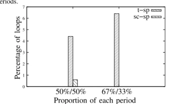
Figure 4. The percentage of loops increases when slow protocols are used for long periods.

Figure 4 shows the percentage of routing loops when the periods are not equal for all the routing protocols.

Instead of only considering the case where p1is equal to

p2(which is denoted by 50%/50%), we also consider the

case where p1 = 2p2 (which is denoted by 67%/33%).

In both cases, the duration of p1+ p2 is constant and

is equal to six hops. The highest percentage of routing loops occurs when the worst protocol in terms of number of hops (either the tree protocol or the shortcut protocol) is given the longest period.

Figure 5 shows the percentage of routing loops as the network density varies from 5 to 33 neighbors per node, with periods lasting for three hops. The percentage of routing loops decreases as the density increases, as nodes have more routing options, and consequently packets are able to reach the destination faster.

2) Imperfect Medium: In this part, we consider that the medium is imperfect: some frames might be dropped due to collisions or bad propagation conditions. Stochastic MAC protocols are included in this case. To model the impact of frame loss, we varied the probability of suc-cessful transmissions at the MAC sub-layer. A sucsuc-cessful transmission rate of 1 corresponds to a perfect medium. The duration of a period becomes the number of attempts to access the medium, and is set to five. Retransmitting a lost frame requires a new transmission attempt. With this setup, infinite routing loops are unlikely because of the randomness of the forwarding. Indeed, for a infinite routing loop to occur, a frame has to reach several times the same node, and to be forwarded each time in the same way (that is, with the same routing protocol). However, because of the imperfect medium, it is likely that some transmission attempts will fail, thus the routing protocol might change for some transmission attempts, which changes the way the frame is forwarded. However, the number of hops experienced by the frames might still be large. Thus, the following simulations focus on the average number of hops rather than on the percentage of routing loops.

Figure 6 shows the average number of hops to reach the destination as a function of the successful transmission rate, for several protocols. As expected, the number of hops decreases when the successful transmission rate increases. The tree protocol is consistently producing the largest number of hops. Shortest path protocols produce the smallest number of hops. The shortcut protocol has an intermediate number of hops. The figure also shows three schedules: the tree protocol with the shortcut protocol, represented by t-sc, the tree protocol with a shortest path protocol, represented by t-sp, and the shortcut protocol with a shortest path protocol, represented by sc-sp. For schedule t-sc, the average number of hops is intermediate between the ones produced by R1 and by R2. For

schedule t-sp, the number of hops is much closer to the number of hops produced by the tree protocol (which is the protocol producing the largest number of hops) than to the number of hops produced by the shortest path protocol, especially when the successful transmission rate is low. Schedule sc-sp has an even worse behavior: the resulting number of hops is on average higher than

00 11 0 0 0 0 1 1 1 1 00 11 00 11 0 0 0 0 0 0 0 0 0 0 0 0 0 0 0 0 1 1 1 1 1 1 1 1 1 1 1 1 1 1 1 1 0 0 0 0 0 0 0 0 0 0 0 0 0 1 1 1 1 1 1 1 1 1 1 1 1 1 0 0 0 0 0 1 1 1 1 1 0 0 0 1 1 1 0 1 0011 t−sp sc−sp 0 2 4 6 8 10 5 9 15 20 27 33 Network density P er ce n ta g e o f lo o p s

Figure 5. The percentage of routing loops decreases as the network density increases. tree (alone) t−sp sc−sp t−sc shortcut (alone) sp−OLSR, shortest (alone)

0 5 10 15 20 25 30 0.2 0.3 0.4 0.5 0.6 0.7 0.8 0.9 1 Successful transmission rate

A v er ag e n u m b er o f h o p s

Figure 6. The average number of hops decreases with the successful transmission rate.

the number of hops produced by the shortcut protocol. This can be explained by the presence of routing loops (although not infinite).

In the following of this section, we show how our proposed 3-step solution impacts the number of hops.

C. Step 1: Compatible Routing Protocols

Figure 7 shows the average number of hops to reach the destination as the density increases, for compatible protocols. Recall that it is not possible to produce a loop with the two chosen schedules. Thus, the average number of hops produced by schedule t-sc (respectively by schedule sp-OLSR) is bounded by the average number of hops produced by the tree and shortcut (resp. shortest path and OLSR) protocols. The number of hops decreases as the density increases: the more neighbors a node has, the smaller is the path to the destination.

tree (alone) t−sc shortcut (alone) sp−OLSR, shortest (alone), OLSR (alone)

1 2 3 4 5 6 7 8 9 5 9 15 20 27 33 Network density A v er ag e n u m b er o f h o p s

Figure 7. Average number of hops as a function of network density.

D. Step 2: Delayable Routing Protocols

Figure 8 shows the average number of hops as a function of the network density, when using delayable

routing protocols, and with dsp as a holding function.

We consider that the number of transmission attempts (and therefore, the number of hops) increases by 1 every time a node decides to hold a packet. This approach does not yield to routing loops. However, the number of hops might exceed the number of hops computed by the worst protocol used alone (which is the tree routing protocol in our case). This is due to the fact that every node computes the distance from its next hop to the destination by using the holding function and the current active routing protocol. If the distance computed by the holding function is the smallest, the node holds the packet and wait until the next routing protocol becomes active, which increases the number of hops.

sc−sp tree (alone) 1 2 3 4 5 6 7 8 9 10 11 5 9 15 20 27 33 t−sp shortcut (alone) shortest (alone) Network density N u m b er o f h o p s (a)

Figure 8. Average number of hops as a function of the network density, using dspas a holding function.

E. Step 3: Combined Routing Protocols

The tree protocol is used as the R∗ _{protocol, and is}

combined with R2 only (to save energy duringR1). The

resulting schedule is modeled by(R1,R2∪R∗). No loop

can appear in the network with such schedules.

Figure 9 shows the average number of hops in terms of the network density for our combined approach, for several schedules. The average number of hops for our combined approach decreases as the network density in-creases. On average, the number of hops for our combined approach is between the number of hops of the two protocols used in the schedule. Moreover, in our simu-lations, the number of hops for our combined approach was always smaller than the largest number of hops of R1 andR2. tree (alone) t−sp t−sc shortcut (alone) sc−sp shortest (alone), sp−OLSR, OLSR (alone)

1 2 3 4 5 6 7 8 9 5 9 15 20 27 33 Network density A v er ag e n u m b er o f h o p s

Figure 9. Average number of hops as a function of network density, with our combined approach, for periods of 3 hops.

VI. CONCLUSION

In order to mitigate the problem of providing several QoS in a network, several pairs of routing and MAC protocols can operate in a scheduled manner in the same network. However, loops can occur if queue exchange is allowed between these pairs. In this paper, we quanti-fied the number and impact of loops in a large variety of scenarios. Then, we proposed a 3-step solution that can be applied to remove loops according to a local decision. Our solution classifies the routing protocols in three categories: compatible routing protocols that cannot yield loops, delayable routing protocols that allow nodes to hold packets in order to avoid loops, and combined routing protocols that allow arbitrary combinations of routing protocols with a known, specific routing protocol. We prove that our solution cannot yield to loops in the network. Then, we proved its performance through extensive simulations.

REFERENCES

[1] X. Carcelle, B. Heile, C. Chatellier, and P. Pailler, “Next WSN applications using ZigBee,” in IFIP Home Networking, vol. 256, 2007, pp. 239–254.

[2] I. F. Akyildiz, X. Wang, and W. Wang, “Wireless mesh networks: a survey,” Computer networks, vol. 47, pp. 445–487, 2005. [3] P. Baronti, P. Pillai, V. W. C. Chook, S. Chessa, A. Gotta, and

Y. Fun Hu, “Wireless sensor networks: A survey on the state of the art and the 802.15.4 and ZigBee standards,” Computer

communications, vol. 30, pp. 1655–1695, 2007.

[4] J. Steffan, L. Fiege, M. Cilia, and A. Buchmann, “Towards multi-purpose wireless sensor networks,” in Systems Communications, 2005, pp. 336–341.

[5] P. J. del Cid, D. Hughes, S. Michiels, and W. Joosen, “Expressing and configuring quality of data in multi-purpose wireless sensor networks,” in Sensor Systems and Software, vol. 57, 2011, pp. 91–106.

[6] L. Song and D. Hatzinakos, Emerging Communications for

Wire-less Sensor Networks. InTech, 2010, ch. Wireless sensor networks: from application specific to modular design, pp. 1–12.

[7] IEEE 802.15, “Part 15.4: Wireless medium access control (MAC) and physical layer (PHY) specifications for low-rate wireless personal area networks (WPANs),” ANSI/IEEE, Standard 802.15.4 R2006, 2006.

[8] I. Rhee, A. Warrier, M. Aia, and J. Min, “Z-MAC: a hybrid MAC protocol for wireless sensor networks,” in ACM SenSys, 2005. [9] G. S. Ahn, E. Miluzzo, A. Campbell, S. Hong, and F. Cuomo,

“Funneling-MAC: a localized, sink oriented MAC for boosting fidelity in sensor networks,” in ACM SenSys, 2006, pp. 293–306. [10] G. Chalhoub, A. Guitton, and M. Misson, “MAC specifications for a WPAN allowing both energy saving and guaranteed delay -Part A: MaCARI: a synchronized tree-based MAC protocol,” in

IFIP WSAN, 2008.

[11] S. Mahfoudh and P. Minet, “EOLSR: an energy efficient routing protocol in wireless ad hoc and sensor networks,” Journal of

Interconnection Networks, vol. 9, no. 4, 2008.

[12] N. El Rachkidy, A. Guitton, and M. Misson, “Improving QoS in Wireless Sensor Networks using a Multi-stack Architecture,” in

IEEE VTC (Vehicular Technology Conference), May 2011. [13] K. Jamieson, D. Moss, and P. Levis, “Collection tree protocol,” in

ACM SenSys, November 2009.

[14] ZigBee, “ZigBee Specification,” ZigBee Standards Organization, Standard Zigbee 053474r17, January 2008.

[15] F. Cuomo, S. Della Luna, U. Monaco, and F. Melodia, “Routing in ZigBee: Benefits from exploiting the IEEE 802.15.4 associa-tion tree,” in IEEE Internaassocia-tional Conference on Communicaassocia-tions

(ICC), 2007, pp. 3271–3276.

[16] T. Kim, D. Kim, N. Park, S.-E. Yoo, and T. S. L ´opez, “Shortcut tree routing in ZigBee networks,” in IEEE ISWPC, February 2007, pp. 42–47.

[17] C. Perkins, E. Belding-Royer, and S. Das, “Ad hoc on-demand distance vector (AODV) routing,” IETF, Request For Comments 3561, July 2003.

[18] C. Adjih, T. Clausen, P. Jacquet, A. Laouiti, P. Minet, P. Muh-lethaler, A. Qayyum, and L. Viennot, “Optimized link state routing protocol,” IETF, RFC 3626, 2003.

[19] N. El Rachkidy, G. Chalhoub, A. Guitton, and M. Misson, “Queue-exchange Mechanism to Improve the QoS in a Multi-stack Archi-tecture,” in ACM PE-WASUN, November 2011.

Nancy El Rachkidy is an assistant professor at Clermont Universit´e, Universit´e Blaise Pascal, France. She is doing her research at LIMOS-CNRS. She received her PhD in 2011 at Uni-versit´e Blaise Pascal. She obtained her MSc degree in networks and computer science from the Lebanese University of Beirut, Lebanon, in 2006. Her research interests include wireless communincations, sensor network, MAC and routing protocols.

Alexandre Guitton is an assistant professor at Clermont Universit´e, Universit´e Blaise Pascal, France. He is doing his research at LIMOS-CNRS. He received his PhD in 2005 and his MSc in 2002 at University of Rennes I, in the field of computer networks. He has been working at Clermont Universit´e since 2007. His research interests include wireless com-munications, sensor networks, MAC protocols, and energy-efficiency.

Michel Misson obtained his PhD thesis in nuclear physics and his ”Habilitation `a Diriger des Recherches” (HDR) degree respectively in 1979 and 2001 both at Universit´e Blaise Pascal, Clermont-Ferrand in France. In 1983, he became a lecturer, teaching networks and system architecture in the Computer Science Department of the institute of Technology in Clermont-Ferrand. He is now Professor in the Networks and Telecommunications De-partment and he manages the research team ”R´eseaux et Protocoles” of the Computer Science Laboratory of Univer-sit´e Blaise Pascal: LIMOS-CNRS. He served on many conference com-mittees and journals reviewing processes. He has also held a visiting po-sition in the research Laboratory T´el´ebec in Underground Communica-tions of Quebec University in Abitibi-Temiscamingue (LRTCS-UQAT). His current research interests are Wireless Local Area Networks, Low Power Wireless Personal Networks, Wireless Sensor Networks real-time systems and protocol engineering.