Latent Semantic Word Sense Induction and Disambiguation

HAL Id: hal-00607672

https://hal.archives-ouvertes.fr/hal-00607672

HAL is a multi-disciplinary open access archive for the deposit and dissemination of sci-entific research documents, whether they are pub-lished or not. The documents may come from teaching and research institutions in France or abroad, or from public or private research centers.

L’archive ouverte pluridisciplinaire HAL, est destinée au dépôt et à la diffusion de documents scientifiques de niveau recherche, publiés ou non, émanant des établissements d’enseignement et de recherche français ou étrangers, des laboratoires publics ou privés.

Latent Semantic Word Sense Induction and

Disambiguation

Tim van de Cruys, Marianna Apidianaki

To cite this version:

Tim van de Cruys, Marianna Apidianaki. Latent Semantic Word Sense Induction and Disambiguation. ACL HLT 2011 - 49th Annual Meeting of the Association for Computational Linguistics: Human Language Technologies, Jun 2011, Portland, Oregon, United States. pp.1476–1485. �hal-00607672�

Latent Semantic Word Sense Induction and Disambiguation

Tim Van de Cruys RCEAL

University of Cambridge United Kingdom tv234@cam.ac.uk

Marianna Apidianaki

Alpage, INRIA & Univ Paris Diderot Sorbonne Paris Cit´e, UMRI-001

75013 Paris, France

marianna.apidianaki@inria.fr

Abstract

In this paper, we present a unified model for the automatic induction of word senses from text, and the subsequent disambiguation of particular word instances using the automati-cally extracted sense inventory. The induction step and the disambiguation step are based on the same principle: words and contexts are mapped to a limited number of topical dimen-sions in a latent semantic word space. The in-tuition is that a particular sense is associated with a particular topic, so that different senses can be discriminated through their association with particular topical dimensions; in a similar vein, a particular instance of a word can be dis-ambiguated by determining its most important topical dimensions. The model is evaluated on theSEMEVAL-2010 word sense induction and disambiguation task, on which it reaches state-of-the-art results.

1 Introduction

Word sense induction (WSI) is the task of automati-cally identifying the senses of words in texts, with-out the need for handcrafted resources or manually annotated data. The manual construction of a sense inventory is a tedious and time-consuming job, and the result is highly dependent on the annotators and the domain at hand. By applying an automatic proce-dure, we are able to only extract the senses that are objectively present in a particular corpus, and it al-lows for the sense inventory to be straightforwardly adapted to a new domain.

Word sense disambiguation (WSD), on the other

hand, is the closely related task of assigning a sense

label to a particular instance of a word in context, using an existing sense inventory. The bulk ofWSD

algorithms up till now use pre-defined sense inven-tories (such as WordNet) that often contain fine-grained sense distinctions, which poses serious prob-lems for computational semantic processing (Ide and Wilks, 2007). Moreover, mostWSDalgorithms take a supervised approach, which requires a signifi-cant amount of manually annotated training data.

The model presented here induces the senses of words in a fully unsupervised way, and subsequently uses the induced sense inventory for the unsuper-vised disambiguation of particular occurrences of words. The induction step and the disambiguation step are based on the same principle: words and contexts are mapped to a limited number of topical dimensions in a latent semantic word space. The key idea is that the model combines tight, synonym-like similarity (based on dependency relations) with broad, topical similarity (based on a large ‘bag of words’ context window). The intuition in this is that the dependency features can be disambiguated by the topical dimensions found by the broad contex-tual features; in a similar vein, a particular instance of a word can be disambiguated by determining its most important topical dimensions (based on the in-stance’s context words).

The paper is organized as follows. Section 2 presents some previous research on distributional similarity and word sense induction. Section 3 gives an overview of our method for word sense induction and disambiguation. Section 4 provides a quantita-tive evaluation and comparison to other algorithms in the framework of theSEMEVAL-2010 word sense

induction and disambiguation (WSI/WSD) task. The last section draws conclusions, and lays out a num-ber of future research directions.

2 Previous Work

2.1 Distributional similarity

According to the distributional hypothesis of mean-ing (Harris, 1954), words that occur in similar con-texts tend to be semantically similar. In the spirit of this by now well-known adage, numerous algo-rithms have sprouted up that try to capture the se-mantics of words by looking at their distribution in texts, and comparing those distributions in a vector space model.

One of the best known models in this respect is latent semantic analysis — LSA(Landauer and

Du-mais, 1997; Landauer et al., 1998). InLSA, a term-document matrix is created, that contains the fre-quency of each word in a particular document. This matrix is then decomposed into three other matrices with a mathematical factorization technique called singular value decomposition (SVD). The most

im-portant dimensions that come out of theSVDare said to represent latent semantic dimensions, according to which nouns and documents can be represented more efficiently. Our model also applies a factoriza-tion technique (albeit a different one) in order to find a reduced semantic space.

Context is a determining factor in the nature of the semantic similarity that is induced. A broad con-text window (e.g. a paragraph or document) yields broad, topical similarity, whereas a small context yields tight, synonym-like similarity. This has lead a number of researchers to use the dependency rela-tions that a particular word takes part in as contex-tual features. One of the most important approaches is Lin (1998). An overview of dependency-based semantic space models is given in Pad´o and Lapata (2007).

2.2 Word sense induction

The following paragraphs provide a succinct overview of word sense induction research. A thor-ough survey on word sense disambiguation (includ-ing unsupervised induction algorithms) is presented in Navigli (2009).

Algorithms for word sense induction can roughly

be divided into local and global ones. Local WSI

algorithms extract the different senses of a word on a per-word basis, i.e. the different senses for each word are determined separately. They can be further subdivided into context-clustering algorithms and graph-based algorithms. In the context-clustering approach, context vectors are created for the differ-ent instances of a particular word, and those con-texts are grouped into a number of clusters, repre-senting the different senses of the word. The con-text vectors may be represented as first or second-order co-occurrences (i.e. the contexts of the target word are similar if the words they in turn co-occur with are similar). The first one to propose this idea of context-group discrimination was Sch¨utze (1998), and many researchers followed a similar approach to sense induction (Purandare and Pedersen, 2004). In the graph-based approach, on the other hand, a co-occurrence graph is created, in which nodes rep-resent words, and edges connect words that appear in the same context (dependency relation or con-text window). The senses of a word may then be discovered using graph clustering techniques (Wid-dows and Dorow, 2002), the HyperLex algorithm (V´eronis, 2004), or Pagerank algorithm (Agirre et al., 2006). Finally, Bordag (2006) recently pro-posed an approach that uses word triplets to per-form word sense induction. The underlying idea is the ‘one sense per collocation’ assumption, and co-occurrence triplets are clustered based on the words they have in common.

Global algorithms take an approach in which the different senses of a particular word are determined by comparing them to, and demarcating them from, the senses of other words in a full-blown word space model. The best known global approach is the one by Pantel and Lin (2002). They present a global clustering algorithm – coined clustering by commit-tee (CBC) – that automatically discovers word senses from text. The key idea is to first discover a set of tight, unambiguous clusters, to which possibly am-biguous words can be assigned. Once a word has been assigned to a cluster, the features associated with that particular cluster are stripped off the word’s vector. This way, less frequent senses of the word may be discovered.

Van de Cruys (2008) proposes a model for sense induction based on latent semantic dimensions.

Us-ing an extension of non-negative matrix factoriza-tion, the model induces a latent semantic space according to which both dependency features and broad contextual features are classified. Using the latent space, the model is able to discriminate be-tween different word senses. The model presented below is an extension of this approach: whereas the model described in Van de Cruys (2008) is only able to perform word sense induction, our model is ca-pable of performing both word sense induction and disambiguation.

3 Methodology

3.1 Non-negative Matrix Factorization

Our model uses non-negative matrix factorization (Lee and Seung, 2000) in order to find latent dimen-sions. There are a number of reasons to preferNMF

over the better known singular value decomposition used in LSA. First of all, NMF allows us to mini-mize the Kullback-Leibler divergence as an objec-tive function, whereasSVDminimizes the Euclidean distance. The Kullback-Leibler divergence is better suited for language phenomena. Minimizing the Eu-clidean distance requires normally distributed data, and language phenomena are typically not normally distributed. Secondly, the non-negative nature of the factorization ensures that only additive and no sub-tractive relations are allowed. This proves partic-ularly useful for the extraction of semantic dimen-sions, so that theNMFmodel is able to extract much more clear-cut dimensions than anSVDmodel. And

thirdly, the non-negative property allows the result-ing model to be interpreted probabilistically, which is not straightforward with anSVDfactorization.

The key idea is that a non-negative matrix A is factorized into two other non-negative matrices, W and H

A_{i×j ≈ Wi×k}H_{k×j (1)}

where k is much smaller than i, j so that both in-stances and features are expressed in terms of a few components. Non-negative matrix factorization en-forces the constraint that all three matrices must be non-negative, so all elements must be greater than or equal to zero.

Using the minimization of the Kullback-Leibler divergence as an objective function, we want to

find the matrices W and H for which the Kullback-Leibler divergence between A and WH (the multipli-cation of W and H) is the smallest. This factoriza-tion is carried out through the iterative applicafactoriza-tion of update rules. Matrices W and H are randomly initialized, and the rules in 2 and 3 are iteratively ap-plied – alternating between them. In each iteration, each vector is adequately normalized, so that all di-mension values sum to 1.

H_{aµ ← Haµ} P iWia A_iµ (WH)iµ P kWka (2) W_{ia← Wia} P µHaµ A_iµ (WH)iµ P vHav (3) 3.2 Word sense induction

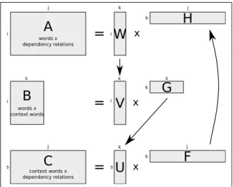
Using an extension of non-negative matrix factoriza-tion, we are able to jointly induce latent factors for three different modes: words, their window-based (‘bag of words’) context words, and their depen-dency relations. Three matrices are constructed that capture the pairwise co-occurrence frequencies for the different modes. The first matrix contains co-occurrence frequencies of words cross-classified by dependency relations, the second matrix contains co-occurrence frequencies of words cross-classified by words that appear in the noun’s context window, and the third matrix contains co-occurrence frequen-cies of dependency relations cross-classified by co-occurring context words. NMFis then applied to the three matrices and the separate factorizations are in-terleaved (i.e. the results of the former factorization are used to initialize the factorization of the next ma-trix). A graphical representation of the interleaved factorization algorithm is given in figure 1.

The procedure of the algorithm goes as follows. First, matrices W, H, G, and F are randomly initial-ized. We then start our first iteration, and compute the update of matrix W (using equation 3). Matrix W is then copied to matrix V, and the update of matrix G is computed (using equation 2). The trans-pose of matrix G is again copied to matrix U, and the update of F is computed (again using equation 2). As a last step, matrix F is copied to matrix H, and we restart the iteration loop until a stopping criterion (e.g. a maximum number of iterations, or no more significant change in objective function; we used the

=

_W

H

=

_V

G

=

_U

F

A

B

C

Figure 1: A graphical representation of the interleaved NMFalgorithm

former one) is reached.1 When the factorization is finished, the three different modes (words, window-based context words and dependency relations) are all represented according to a limited number of la-tent factors.

Next, the factorization that is thus created is used for word sense induction. The intuition is that a par-ticular, dominant dimension of an ambiguous word is ‘switched off’, in order to reveal other possible senses of the word. Formally, we proceed as follows. Matrix H indicates the importance of each depen-dency relation given a topical dimension. With this knowledge, the dependency relations that are respon-sible for a certain dimension can be subtracted from the original noun vector. This is done by scaling down each feature of the original vector according to the load of the feature on the subtracted dimen-sion, using equation 4.

t_{= v(u}1− hk) (4)

Equation 4 multiplies each dependency feature of the original noun vector v with a scaling factor, ac-cording to the load of the feature on the subtracted dimension (hk – the vector of matrix H that

corre-sponds to the dimension we want to subtract). u1is

a vector of ones with the same length as hk. The

re-sult is vector t, in which the dependency features

rel-1

Note that this is not the only possibly way of interleaving the different factorizations, but in our experiments we found that different constellations lead to similar results.

evant to the particular topical dimension have been scaled down.

In order to determine which dimension(s) are re-sponsible for a particular sense of the word, the method is embedded in a clustering approach. First, a specific word is assigned to its predominant sense (i.e. the most similar cluster). Next, the dominant semantic dimension(s) for this cluster are subtracted from the word vector, and the resulting vector is fed to the clustering algorithm again, to see if other word senses emerge. The dominant semantic dimen-sion(s) can be identified by folding vector c – repre-senting the cluster centroid – into the factorization (equation 5). This yields a probability vector b over latent factors for the particular centroid.

b_{= cH}T ₍₅₎

A simple k-means algorithm is used to com-pute the initial clustering, using the non-factorized dependency-based feature vectors (matrix A). k-means yields a hard clustering, in which each noun is assigned to exactly one (dominant) cluster. In the second step, it is determined for each noun whether it can be assigned to other, less dominant clusters. First, the salient dimension(s) of the centroid to which the noun is assigned are determined. The cen-troid of the cluster is computed by averaging the fre-quencies of all cluster elements except for the tar-get word we want to reassign. After subtracting the salient dimensions from the noun vector, it is checked whether the vector is reassigned to another cluster centroid. If this is the case, (another instance of) the noun is assigned to the cluster, and the sec-ond step is repeated. If there is no reassignment, we continue with the next word. The target element is removed from the centroid to make sure that only the dimensions associated with the sense of the cluster are subtracted. When the algorithm is finished, each noun is assigned to a number of clusters, represent-ing its different senses.

We use two different methods for selecting the fi-nal number of candidate senses. The first method, NMFcon, takes a conservative approach, and only

selects candidate senses if – after the subtraction of salient dimensions – another sense is found that is more similar to the adapted noun vector. The second method, NMFlib, is more liberal, and also selects the

next best cluster centroid as candidate sense until a certain similarity threshold φ is reached.2

3.2.1 Word sense disambiguation

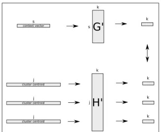
The sense inventory that results from the induc-tion step can now be used for the disambiguainduc-tion of individual instances as follows. For each instance of the target noun, we extract its context words, i.e. the words that co-occur in the same paragraph, and rep-resent them as a probability vector f . Using matrix G from our factorization model (which represents context words by semantic dimensions), this vector can be folded into the semantic space, thus represent-ing a probability vector over latent factors for the particular instance of the target noun (equation 6).

d_{= fG}T ₍₆₎

Likewise, the candidate senses of the noun (repre-sented as centroids) can be folded into our seman-tic space using matrix H (equation 5). This yields a probability distribution over the semantic dimen-sions for each centroid. As a last step, we com-pute the Kullback-Leibler divergence between the context vector and the candidate centroids, and se-lect the candidate centroid that yields the lowest di-vergence as the correct sense. The disambiguation process is represented graphically in figure 2.

G'

H'

Figure 2: Graphical representation of the disambiguation process

2_{Experimentally (examining the cluster output), we set φ =}

0_.2

3.2.2 Example

Let us clarify the process with an example for the noun chip. The sense induction algorithm finds the following candidate senses:3

1. cache, CPU, memory, microprocessor, proces-sor, RAM, register

2. bread, cake, chocolate, cookie, recipe, sand-wich

3. accessory, equipment, goods, item, machinery, material, product, supplies

Each candidate sense is associated with a centroid (the average frequency vector of the cluster’s mem-bers), that is folded into the semantic space, which yields a ‘semantic fingerprint’, i.e. a distribution over the semantic dimensions. For the first sense, the ‘computer’ dimension will be the most impor-tant. Likewise, for the second and the third sense the ‘food’ dimension and the ‘manufacturing’ dimension

will be the most important.4

Let us now take a particular instance of the noun chip, such as the one in (1).

(1) An N.V. Philips unit has created a com-puter system that processes video images 3,000 times faster than conventional systems. Using reduced instruction - set comput-ing, or RISC, chips made by Intergraph of Huntsville, Ala., the system splits the im-age it ‘sees’ into 20 digital representations, each processed by one chip.

Looking at the context of the particular instance of chip, a context vector is created which represents the semantic content words that appear in the same paragraph (the extracted content words are printed in boldface). This context vector is again folded into the semantic space, yielding a distribution over the semantic dimensions. By selecting the lowest Kullback-Leibler divergence between the semantic probability distribution of the target instance and the

3_{Note that we do not use the word sense to hint at a}

lexico-graphic meaning distinction; rather, sense in this case should be regarded as a more coarse-grained and topic-related entity.

4

In the majority of cases, the induced dimensions indeed contain such clear-cut semantics, so that the dimensions can be rightfully labeled as above.

semantic probability distributions of the candidate senses, the algorithm is able to assign the ‘computer’ sense of the target noun chip.

4 Evaluation

4.1 Dataset

Our word sense induction and disambiguation model is trained and tested on the dataset of the

SEMEVAL-2010 WSI/WSD task (Manandhar et al.,

2010). TheSEMEVAL-2010WSI/WSDtask is based on a dataset of 100 target words, 50 nouns and 50 verbs. For each target word, a training set is pro-vided from which the senses of the word have to be induced without using any other resources. The training set for a target word consists of a set of target word instances in context (sentences or para-graphs). The complete training set contains 879,807 instances, viz. 716,945 noun and 162,862 verb in-stances.

The senses induced during training are used for disambiguation in the testing phase. In this phase, the system is provided with a test set that consists of unseen instances of the target words. The test set contains 8,915 instances in total, of which 5,285 noun and 3,630 verb instances. The instances in the test set are tagged with OntoNotes senses (Hovy et al., 2006). The system needs to disambiguate these instances using the senses acquired during training. 4.2 Implementational details

The SEMEVAL training set has been part of speech

tagged and lemmatized with the Stanford Part-Of-Speech Tagger (Toutanova and Manning, 2000; Toutanova et al., 2003) and parsed with Malt-Parser (Nivre et al., 2006), trained on sections 2-21 of the Wall Street Journal section of the Penn Treebank extended with about 4000 questions from the QuestionBank5 in order to extract dependency triples. TheSEMEVALtest set has only been tagged and lemmatized, as our disambiguation model does not use dependency triples as features (contrary to the induction model).

We constructed two different models – one for nouns and one for verbs. For each model, the matri-ces needed for our interleavedNMFfactorization are

5_{http://maltparser.org/mco/english_}

parser/engmalt.html

extracted from the corpus. The noun model was built using 5K nouns, 80K dependency relations, and 2K

context words (excluding stop words) with highest frequency in the training set, which yields matrices of 5Knouns× 80Kdependency relations, 5Knouns

× 2Kcontext words, and 80Kdependency relations × 2Kcontext words. The model for verbs was con-structed analogously, using 3K verbs, and the same

number of dependency relations and context words. For our initial k-means clustering, we set k = 600 for nouns, and k = 400 for verbs. For the under-lying interleavedNMFmodel, we used 50 iterations, and factored the model to 50 dimensions.

4.3 Evaluation measures

The results of the systems participating in the

SEMEVAL-2010 WSI/WSD task are evaluated both

in a supervised and in an unsupervised manner. The supervised evaluation in theSEMEVAL-2010

WSI/WSDtask follows the scheme of theSEMEVAL

-2007WSItask (Agirre and Soroa, 2007), with some modifications. One part of the test set is used as a mapping corpus, which maps the automatically in-duced clusters to gold standard senses; the other part acts as an evaluation corpus. The mapping between clusters and gold standard senses is used to tag the evaluation corpus with gold standard tags. The sys-tems are then evaluated as in a standard WSD task, using recall.

In the unsupervised evaluation, the induced senses are evaluated as clusters of instances which are compared to the sets of instances tagged with the gold standard senses (corresponding to classes). Two partitions are thus created over the test set of a target word: a set of automatically generated clus-ters and a set of gold standard classes. A number of these instances will be members of both one gold standard class and one cluster. Consequently, the quality of the proposed clustering solution is evalu-ated by comparing the two groupings and measuring their similarity.

Two evaluation metrics are used during the unsu-pervised evaluation in order to estimate the quality of the clustering solutions, the V-Measure (Rosen-berg and Hirsch(Rosen-berg, 2007) and the paired F-Score(Artiles et al., 2009). V-Measure assesses the quality of a clustering by measuring its homogeneity (h) and its completeness (c). Homogeneity refers to

the degree that each cluster consists of data points primarily belonging to a single gold standard class, while completeness refers to the degree that each gold standard class consists of data points primarily assigned to a single cluster. V-Measure is the har-monic mean of h and c.

V M = 2 · h · c

h+ c (7)

In the paired F-Score (Artiles et al., 2009) eval-uation, the clustering problem is transformed into a classification problem (Manandhar et al., 2010). A set of instance pairs is generated from the automati-cally induced clusters, which comprises pairs of the instances found in each cluster. Similarly, a set of in-stance pairs is created from the gold standard classes, containing pairs of the instances found in each class. Precisionis then defined as the number of common instance pairs between the two sets to the total num-ber of pairs in the clustering solution (cf. formula 8). Recallis defined as the number of common instance pairs between the two sets to the total number of pairs in the gold standard (cf. formula 9). Preci-sion and recall are finally combined to produce the harmonic mean (cf. formula 10).

P = |F (K) ∩ F (S)| |F (K)| (8) R= |F (K) ∩ F (S)| |F (S)| (9) F S= 2 · P · R P + R (10)

The obtained results are also compared to two baselines. The most frequent sense (MFS) baseline groups all testing instances of a target word into one cluster. The Random baseline randomly assigns an instance to one of the clusters.6 This baseline is exe-cuted five times and the results are averaged.

4.4 Results

4.4.1 Unsupervised evaluation

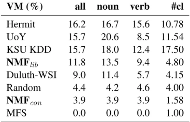
In table 1, we present the performance of a num-ber of algorithms on the V-measure. We compare

6

The number of clusters in Random was chosen to be roughly equal to the average number of senses in the gold stan-dard.

our V-measure scores with the scores of the best-ranked systems in the SEMEVAL 2010 WSI/WSD

task, both for the complete data set and for nouns and verbs separately. The fourth column shows the average number of clusters induced in the test set by each algorithm. TheMFSbaseline has a V-Measure equal to 0, since by definition its completeness is 1 and its homogeneity is 0.

NMFcon– our model that takes a conservative

ap-proach in the induction of candidate senses – does not beat the random baseline. NMFlib – our model

that is more liberal in inducing senses – reaches bet-ter results. With 11.8%, it scores similar to other algorithms that induce a similar average number of clusters, such as Duluth-WSI (Pedersen, 2010).

Pedersen (2010) has shown that the V-Measure tends to favour systems producing a higher number of clusters than the number of gold standard senses. This is reflected in the scores of our models as well.

VM (%) all noun verb #cl

Hermit 16.2 16.7 15.6 10.78 UoY 15.7 20.6 8.5 11.54 KSU KDD 15.7 18.0 12.4 17.50 NMFlib 11.8 13.5 9.4 4.80 Duluth-WSI 9.0 11.4 5.7 4.15 Random 4.4 4.2 4.6 4.00 NMFcon 3.9 3.9 3.9 1.58 MFS 0.0 0.0 0.0 1.00

Table 1: unsupervised V-measure evaluation on SE-MEVALtest set

Motivated by the large divergences in the sys-tem rankings on the different metrics used in the

SEMEVAL-2010 WSI/WSD task, Pedersen (2010)

performed an evaluation of the metrics themselves. His evaluation relied on the assumption that a good measure should assign low scores to random base-lines. Pedersen showed that the V-Measure contin-ued to improve as randomness increased. We agree with Pedersen’s conclusion that the V-Measure re-sults should be interpreted with caution, but we still report the results in order to perform a global com-parison, on all metrics, of our system’s performance to the systems that participated to theSEMEVALtask. Contrary to V-Measure, paired F-score is a fairly reliable measure and the only one that managed to

identify and expose random baselines in the above mentioned metric evaluation. This means that the random systems used for testing were ranked low when a high number of random senses was used.

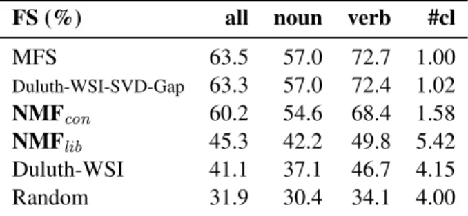
In table 2, the paired F-Score of a number of al-gorithms is given. The paired F-Score penalizes sys-tems when they produce a higher number of clusters (low recall) or a lower number of clusters (low pre-cision) than the gold standard number of senses. We again compare our results with the scores of the best-ranked systems in the SEMEVAL-2010 WSI/WSD

TASK.

FS (%) all noun verb #cl

MFS 63.5 57.0 72.7 1.00 Duluth-WSI-SVD-Gap 63.3 57.0 72.4 1.02 NMFcon 60.2 54.6 68.4 1.58 NMFlib 45.3 42.2 49.8 5.42 Duluth-WSI 41.1 37.1 46.7 4.15 Random 31.9 30.4 34.1 4.00

Table 2: Unsupervised paired F-score evaluation on SE-MEVALtestset

NMFconreaches a score of 60.2%, which is again

similar to other algorithms that induce the same aver-age number clusters. NMFlib scores 45.3%,

indicat-ing that the algorithm is able to retain a reasonable F-Score while at the same time inducing a significant number of clusters. This especially becomes clear when comparing its score to the other algorithms. 4.4.2 Supervised evaluation

In the supervised evaluation, the automatically in-duced clusters are mapped to gold standard senses, using the mapping corpus (i.e. one part of the test set). The obtained mapping is used to tag the evalu-ation corpus (i.e. the other part of the test set) with gold standard tags, which means that the methods are evaluated in a standard WSD task.

Table 3 shows the recall of our algorithms in the supervised evaluation, again compared to other algo-rithms evaluated in the SEMEVAL-2010 WSI/WSD

task.

NMFlib gets 62.6%, which makes it the best

scor-ing algorithm on the supervised evaluation. NMFcon

reaches 60.3%, which again indicates that it is in the

SR (%) all noun verb #S

NMFlib 62.6 57.3 70.2 1.82 UoY 62.4 59.4 66.8 1.51 Duluth-WSI 60.5 54.7 68.9 1.66 NMFcon 60.3 54.5 68.8 1.21 MFS 58.7 53.2 66.6 1.00 Random 57.3 51.5 65.7 1.53

Table 3: Supervised recall for SEMEVAL testset, 80% mapping, 20% evaluation

same ballpark as other algorithms that induce a sim-ilar average number of senses.

Some doubts have been cast on the representative-ness of the supervised recall results as well. Accord-ing to Pedersen (2010), the supervised learnAccord-ing al-gorithm that underlies this evaluation method tends to converge to the Most Frequent Sense (MFS) base-line, because the number of senses that the classi-fier assigns to the test instances is rather low. We think these shortcomings indicate the need for the development of new evaluation metrics, capable of providing a more accurate evaluation of the perfor-mance of WSI systems. Nevertheless, these metrics still constitute a useful testbed for comparing the per-formance of different systems.

5 Conclusion and future work

In this paper, we presented a model based on latent semantics that is able to perform word sense induc-tion as well as disambiguainduc-tion. Using latent topi-cal dimensions, the model is able to discriminate be-tween different senses of a word, and subsequently disambiguate particular instances of a word. The evaluation results indicate that our model reaches state-of-the-art performance compared to other sys-tems that participated in theSEMEVAL-2010 word sense induction and disambiguation task. Moreover, our global approach is able to reach similar perfor-mance on an evaluation set that is tuned to fit the needs of local approaches. The evaluation set con-tains an enormous amount of contexts for only a small number of target words, favouring methods that induce senses on a per-word basis. A global ap-proach like ours is likely to induce a more balanced sense inventory using a more balanced, unbiased

corpus, and is likely to outperform local methods when such an unbiased corpus is used as input. We therefore think that the global, unified approach to word sense induction and disambiguation presented here provides a genuine and powerful solution to the problem at hand.

We conclude with some issues for future work. First of all, we would like to evaluate the approach presented here using a more balanced and unbiased corpus, and compare its performance on such a cor-pus to local approaches. Secondly, we would also like to include grammatical dependency information in the disambiguation step of the algorithm. For now, the disambiguation step only uses a word’s context words; enriching the feature set with dependency in-formation is likely to improve the performance of the disambiguation.

Acknowledgments

This work is supported by the Scribo project, funded by the French ‘pˆole de comp´etitivit´e’ System@tic, and by the French national grant EDyLex (ANR-09-CORD-008).

References

Eneko Agirre and Aitor Soroa. 2007. SemEval-2007 Task 02: Evaluating word sense induction and discrim-ination systems. In Proceedings of the fourth Interna-tional Workshop on Semantic Evaluations (SemEval), ACL, pages 7–12, Prague, Czech Republic.

Eneko Agirre, David Mart´ınez, Ojer L´opez de Lacalle, and Aitor Soroa. 2006. Two graph-based algo-rithms for state-of-the-art WSD. In Proceedings of the Conference on Empirical Methods in Natural Lan-guage Processing (EMNLP-06), pages 585–593, Syd-ney, Australia.

Marianna Apidianaki and Tim Van de Cruys. 2011. A Quantitative Evaluation of Global Word Sense Induc-tion. In Proceedings of the 12th International Con-ference on Intelligent Text Processing and Computa-tional Linguistics (CICLing), published in Springer Lecture Notes in Computer Science (LNCS), volume 6608, pages 253–264, Tokyo, Japan.

Javier Artiles, Enrique Amig´o, and Julio Gonzalo. 2009. The role of named entities in web people search. In Proceedings of the Conference on Empirical Methods in Natural Language Processing (EMNLP-09), pages 534–542, Singapore.

Stefan Bordag. 2006. Word sense induction: Triplet-based clustering and automatic evaluation. In Proceed-ings of the 11th Conference of the European Chap-ter of the Association for Computational Linguistics (EACL-06), pages 137–144, Trento, Italy.

Zellig S. Harris. 1954. Distributional structure. Word, 10(23):146–162.

Eduard Hovy, Mitchell Marcus, Martha Palmer, Lance Ramshaw, and Ralph Weischedel. 2006. Ontonotes: the 90% solution. In Proceedings of the Human Lan-guage Technology / North American Association of Computational Linguistics conference (HLT-NAACL-06), pages 57–60, New York, NY.

Nancy Ide and Yorick Wilks. 2007. Making Sense About Sense. In Eneko Agirre and Philip Edmonds, editors, Word Sense Disambiguation, Algorithms and Applica-tions, pages 47–73. Springer.

Thomas Landauer and Susan Dumais. 1997. A solution to Plato’s problem: The Latent Semantic Analysis the-ory of the acquisition, induction, and representation of knowledge. Psychology Review, 104:211–240. Thomas Landauer, Peter Foltz, and Darrell Laham. 1998.

An Introduction to Latent Semantic Analysis. Dis-course Processes, 25:295–284.

Daniel D. Lee and H. Sebastian Seung. 2000. Algo-rithms for non-negative matrix factorization. In Ad-vances in Neural Information Processing Systems, vol-ume 13, pages 556–562.

Dekang Lin. 1998. Automatic Retrieval and Clustering of Similar Words. In Proceedings of the 36th Annual Meeting of the Association for Computational Linguis-tics and 17th International Conference on Computa-tional Linguistics (COLING-ACL98), volume 2, pages 768–774, Montreal, Quebec, Canada.

Suresh Manandhar, Ioannis P. Klapaftis, Dmitriy Dligach, and Sameer S. Pradhan. 2010. SemEval-2010 Task 14: Word Sense Induction & Disambiguation. In Pro-ceedings of the fifth International Workshop on Seman-tic Evaluation (SemEval), ACL-10, pages 63–68, Upp-sala, Sweden.

Roberto Navigli. 2009. Word Sense Disambiguation: a Survey. ACM Computing Surveys, 41(2):1–69. Joakim Nivre, Johan Hall, and Jens Nilsson. 2006.

Malt-parser: A data-driven parser-generator for dependency parsing. In Proceedings of the fifth International Conference on Language Resources and Evaluation (LREC-06), pages 2216–2219, Genoa, Italy.

Sebastian Pad´o and Mirella Lapata. 2007. Dependency-based construction of semantic space models. Compu-tational Linguistics, 33(2):161–199.

Patrick Pantel and Dekang Lin. 2002. Discovering word senses from text. In ACM SIGKDD International Con-ference on Knowledge Discovery and Data Mining, pages 613–619, Edmonton, Alberta, Canada.

Ted Pedersen. 2010. Duluth-WSI: SenseClusters Ap-plied to the Sense Induction Task of SemEval-2. In Proceedings of the fifth International Workshop on Se-mantic Evaluations (SemEval-2010), pages 363–366, Uppsala, Sweden.

Amruta Purandare and Ted Pedersen. 2004. Word Sense Discrimination by Clustering Contexts in Vec-tor and Similarity Spaces. In Proceedings of the Con-ference on Computational Natural Language Learning (CoNLL), pages 41–48, Boston, MA.

Andrew Rosenberg and Julia Hirschberg. 2007. V-measure: A conditional entropy-based external clus-ter evaluation measure. In Proceedings of the Joint 2007 Conference on Empirical Methods in Natural Language Processing and Computational Natural Lan-guage Learning (EMNLP-CoNLL), pages 410–420, Prague, Czech Republic.

Hinrich Sch¨utze. 1998. Automatic Word Sense Discrim-ination. Computational Linguistics, 24(1):97–123. Kristina Toutanova and Christopher D. Manning. 2000.

Enriching the Knowledge Sources Used in a Maxi-mum Entropy Part-of-Speech Tagger. In Proceedings of the Joint SIGDAT Conference on Empirical Meth-ods in Natural Language Processing and Very Large Corpora (EMNLP/VLC-2000), pages 63–70.

Kristina Toutanova, Dan Klein, Christopher Manning, and Yoram Singer. 2003. Feature-Rich Part-of-Speech Tagging with a Cyclic Dependency Network. In Proceedings of the Human Language Technology / North American Association of Computational Lin-guistics conference (HLT-NAACL-03, pages 252–259, Edmonton, Canada.

Tim Van de Cruys. 2008. Using Three Way Data for Word Sense Discrimination. In Proceedings of the 22nd International Conference on Computational Lin-guistics (COLING-08), pages 929–936, Manchester, UK.

Jean V´eronis. 2004. Hyperlex: lexical cartography for information retrieval. Computer Speech & Language, 18(3):223–252.

Dominic Widdows and Beate Dorow. 2002. A Graph Model for Unsupervised Lexical Acquisition. In Pro-ceedings of the 19th International Conference on Com-putational Linguistics (COLING-02), pages 1093– 1099, Taipei, Taiwan.