Appendix S1 Phylogenetic analyses and species sampling, patterns of lineage diversification and morphological evolution through time
Our nuclear sampling consisted of 18 of 20 extant parrotbill species and different subspecies for several polytypic species, following the taxonomy of Robson (2007) with the exception of Paradoxornis margaritae and P. przewalskii (Table S1). Panurus biarmicus has for a long time been included in Paradoxornithidae (Robson, 2007), but has been recently shown to be only distantly related to this clade (Alström et al., 2006). Hence, it was not included in our analyses.
It should be taken into account that some of the allopatric populations of different parrotbill species have recently been upgraded from subspecies to species based on morphological features (Penhallurick & Robson, 2009; Gill, 2014). This increased species number, however, would have no influence on our conclusions on diversification patterns. First, it would not alter our inferences on morphological evolution because subspecies differ mainly in plumage patterns and not in size and structure. Second, we assume no influence on our conclusions on the history of climate niche evolution, because the split of subspecies to species only concerns recent events and hence merely affects very young clades. Biogeographic inferences could be more resolved towards the present however, but it would not change the results for deeper nodes.
We used DNA sequences for the different species of the two mitochondrial genes cytochrome b (cytb, 1042 base pairs (bp)) and NADH dehydrogenase subunit 2 (ND2, 1041 bp), and two nuclear loci, the nuclear recombination activating gene 1 (RAG1, 962 bp), and the nuclear intron 2 of archain (ARCN1, 742 bp), and the Z-linked intron 5 of ADAM metal lopeptidase with thrombospondin type 1 motif, 6 variant 2 (ADAMTS6, 550 bp). These sequences were retrieved from Yeung et al. (2011). The overall dataset contained 4337 bp for each species. Sequences of the different markers were aligned using the MAFFT algorithm (Katoh et al., 2002) as implemented in GeneiousPro 7.0.6 (Drummond et al., 2011). To infer a species tree from the five analyzed markers, we used the multispecies coalescent algorithm *BEAST as implemented in BEAST 1.7.5 (Drummond & Rambaut, 2007; Heled & Drummond, 2010). The different species and their subspecies were defined a priori as ‘species’ following the
taxonomy of Robson (2007). We used different substitution, clock and tree models for the three nuclear markers, while the two mtDNA markers were assigned the same substitution, clock and tree model. Best-fitting substitution models were evaluated with Modeltest (Posada & Crandall, 1998), as implemented in GeneiousPro. A Yule process on species trees was implemented in all analyses, and we used a relaxed uncorrelated lognormal distribution for the different partitions. To calibrate the species tree, we implemented a substitution rate for the mtDNA, using the robust overall divergence rate of 2.1 per million year (Ma) (0.0105 substitution/site/Ma)(Weir & Schluter, 2008), of 0.00135 substitution/site/Ma for the two nuclear markers (Ellegren, 2007; Smith et al., 2013) and of 0.00145 substitution/site/Ma for the sex-linked marker (Ellegren, 2007). These values were used as means for a lognormal prior distribution with a wide logarithmic standard deviation of 0.2. The MCMC analysis was run five times independently for 50 million generations with sampling every 1000 generations. TRACER 1.5 (Rambaut & Drummond, 2007) was used to confirm appropriate burn-in and the adequate effective sample sizes (ESS) of the posterior distribution, and to compare likelihoods and posterior probabilities of all parameters to assess convergence among the five independent runs. The log and tree files from the different runs were combined with LogCombiner 1.7.5 with a burn-in of 15 million generations each. The resulting maximum clade credibility species tree and the 95% highest posterior density (HPD) distributions of each estimated node were calculated with Tree Annotator 1.7.5 (Drummond & Rambaut, 2007) and visualized using FIGTREE 1.2. (Rambaut, 2008).
The comparison of the five independent *BEAST runs revealed convergence of all parameters. When combined with a 15 million generations burn-in each, the resulting effective sample sizes for parameters were > 200, with the exception of five population size parameters with effective sample sizes between 117 and 174. The maximum clade credibility species tree was then computed from 175,005 trees (Fig. 2).
The R packages ‘Laser’ v. 2.4.1 (Rabosky, 2006a), ‘Geiger’ v. 2.0.1 and v. 1.99-3 (Harmon et al., 2008) and ‘Phytools’ 0.9-93 (Revell, 2012) were used for all comparative data modeling. Temporal variation in diversification rates within parrotbills was visualized with semi logarithmic lineage-through-time plots (LTT). We used the mean from the posterior
distribution of trees from the *BEAST analyses and plotted the 95% confidence interval of the lineages given at a time in the past from 1000 trees randomly chosen from the posterior distribution of the *BEAST analyses.
To test whether diversification rates have decreased over time, we calculated the gamma (γ) statistic of Pybus & Harvey (2000). The sensitivity of the inferred gamma value was assessed with the Monte Carlo Constant rate test (MCCR), based on 10, 000 simulated phylogenies, taking into account incomplete taxon sampling.
Different likelihood models for diversification rates were moreover fitted on the maximum clade credibility species tree from the *BEAST analyses (Rabosky, 2006b; Rabosky & Lovette, 2008) (Table 1). AIC (Akaike information criterion) scores were compared among the following models: 1) a pure birth (Yule); 2) birth-death (bd); 3) bd rate-variable model with the speciation rate λ1 shifting to λ2 at a time t (yule2rate); 4) yule3rate; 5) a yule4rate; 6)
exponential diversity-dependent (DDX) and 7) logistic diversity-dependent (DDL) speciation rate model; 8) model with exponentially declining speciation rate through time (constant extinction, SPVAR); 9) exponentially increasing extinction rate through time (constant speciation, EXVAR); 10) varying speciation and extinction rates through time (BOTHVAR). An increase in model fit was overall considered as significant when the reduction in AIC score in a more complex model was ≥ 2 (Burnham & Anderson, 2002).
The gamma (γ) statistic was -1.458 with a P-value of 0.095, as assessed with the Monte Carlo Constant Rate test (MCCR). Hence, we detected no evidence for a significant slowdown of diversification rate over time.
A yule2rate model was found to be the best-fitting model of lineage diversification, with a slight increase in speciation rate shortly before the present when considering ΔAIC, and was significantly different against an overall constant diversification rate over time (Table S3). When considering ΔAICc instead, a DDX model was found to be best fitting, although it was not significantly different from a pure birth model.
We additionally fitted six likelihood models of continuous morphological evolution to our data and compared their AIC scores, based on the maximum clade credibility species tree. The models were: 1) Brownian motion (BM); 2) Ornstein-Uhlenbeck (OU) (Butler & King, 2004); 3)
a time-dependent linear model (TDL), with linear rate change through time; 4) time-dependent early-burst (EB) model, with exponential rate change through time (Harmon et al., 2010); 5) a diversity-dependent linear model (DDL), with its rate changing linearly with changing species diversity in a clade (Weir & Mursleen, 2012); 6) a diversity-dependent linear model (DDX), with its rate changing exponentially with changing species diversity in a clade (Weir & Mursleen, 2012).
Appendix S2 Ecological niche modeling and niche overlaps and equivalency
Occurrence records of each parrotbill species were obtained from two sources: 1) field observation records from the online database “China Bird Report” (http://www.birdreport.cn/) and Li et al. (2013); 2) occurrences from the Global Biodiversity Information Facility database (GBIF; http://www.gbif.org/). All records were mapped using ArcGIS 9.2 (ESRI, Redland, CA) for visual inspection. We detected duplicates and possible errors in georeferencing by double-checking in spreadsheets and geographic information systems (GIS). Because models using only presence data can be affected by sample selection bias (Phillips et al., 2009) and spatial autocorrelation, we created a 0.1°-resolution grid in which we included only a single randomly selected occurrence per grid-cell. This spatial filtering yielded 1, 260 unique georeferenced records from throughout the entire distribution ranges of all species. This stratification enhanced our ability to model the unbiased potential distribution of species and avoided a prediction biased by sampling effort (Soberon & Nakamura, 2009). Consequently, the number of occurrences per species ranged from 1 (P. przewalskii) to 715 (P. webbianus). P. przewalskii and P. flavirostris (N = 3) were excluded when ecological niche models (ENMs) were constructed, due to the small sample size of occurrences.
We obtained 19 bioclimatic variables, representing climatic conditions (the period 1950-2000) within the study area with a resolution of 0.1 arc-degrees from the WorldClim database v.1.4 (Hijmans et al., 2005). Including all bioclimatic variables in ENMs might cause ‘over-fitting’ problems and uncertainties due to high degrees of co-linearity among variables, especially for small sample sizes of occurrences (Heikkinen et al., 2006; Hu & Jiang, 2010). Therefore, we
first carried out Pearson’s correlation tests and jackknife analyses in ENM, and retained the variables that gave a higher value in the percent contribution to the Maxent model (Phillips et al., 2006; Hu & Liu, 2014) for highly correlated variable pairs (|r| ≥ 0.8). Consequently, seven variables were retained as predictors for further analyses: annual mean temperature (Tanu), mean monthly temperature range (Tran), temperature seasonality (Tsea), annual precipitation (Precanu), precipitation in the driest month (Precdry), precipitation seasonality (Precsea), precipitation in the coldest quarter (Preccol).
We used the maximum entropy algorithm employed in Maxent 3.3.3k (Phillips et al., 2006) to construct ENMs for each species. Discrimination abilities of the ENMs were assessed by computing the area under the receiver operating characteristic curve (AUC) (Swets, 1988). We mainly employed default settings and ran models with 10 bootstrap replicates, using 70% of the occurrences for model training and 30% for testing the resulting models. To provide robust projections in climatic suitability, the replicates from Maxent were used as proxy-models to constitute the consensus-based ensemble-forecasting (Araujo & New, 2007). The averages across all replicates were obtained for further processing by calculating within each grid-cell in ArcGIS 9.2 (ESRI, Redland, CA). An easily interpretable logistic output format was selected with suitability values ranging from 0 (lowest) to 1 (highest) (Phillips & Dudik, 2008). To evaluate the niche overlap between species, we calculated two indices, i.e. Schoener's D and I (Warren et al. 2008). These values measured the similarity of projected suitability for each grid cell of the study area and ranged from 0 (no niche overlap) to 1 (complete overlap). The estimates of D and I were obtained by comparing projected suitability from Maxent for each grid cell of the study area, after normalizing each ENM (Warren et al., 2008). We used a niche identity test to test if ENMs of species are distributed in identical environmental space (Warren et al., 2008). We pooled occurrences and randomized their identities by 100 replicates to produce two new samples with the same number of observations as the empirical data. This helped to generate a pseudo-replicated null distribution. The observed similarity values were compared with this null distribution of values of random replicates to determine whether species are more different than would be expected by chance. The null hypothesis of niche identity is rejected when the empirically observed value for D or I is
significantly different from the pseudo-replicated data sets. We calculated the values of D and I in ENMTools 1.3 (Warren et al., 2008, 2010).
References
Alström, P., Ericson, P.G.P., Olsson, U. & Sundberg, P. (2006) Phylogeny and classification of the avian superfamily Sylvioidea. Molecular Phylogenetics and Evolution, 38, 381-397.
Araujo, M.B. & New, M. (2007) Ensemble forecasting of species distributions. Trends in Ecology and Evolution, 22, 42-47.
Baur, H. & Leuenberger, C. (2011) Analysis of ratios in multivariate morphometry. Systematic Biology, 60, 813-825.
Burnham, K.P. & Anderson, D.R. (2002) Model selection and mulitimodel inference (2nd edition).. Springer-Verlag, New York.
Drummond, A.J. & Rambaut, A. (2007) BEAST: Bayesian evolutionary analysis by sampling trees. BMC Evolutionary Biology, 7, 214.
Drummond, A.J., Ashton, B., Buxton, S., Cheung, M., Cooper, A., Duran, C., Field, M., Heled, J., Kearse, M., Markowitz, S., Moir, R., Stones-Havas, S., Sturrock, S., Thierer, T. & Wilson, A. (2011) Geneious v5.4. Available from: http://www.geneious.com/.
Ellegren, H. (2007) Molecular evolutionary genomics of birds. Cytogenetic and Genome Research, 117, 120-130.
Harmon, L.J., Weir, J.T., Brock, C.D., Glor, R.E. & Challenger, W. (2008) GEIGER: investigating evolutionary radiations. Bioinformatics, 24, 129-131.
Heikkinen, R.K., Luoto, M., Araujo, M.B., Virkkala, R., Thuiller, W. & Sykes, M.T. (2006) Methods and uncertainties in bioclimatic envelope modelling under climate change. Progress in Physical Geography, 30, 751-777.
Heled, J. & Drummond, A.J. (2010) Bayesian inference of species trees from multilocus data. Molecular Biology and Evolution, 27, 570-580.
Hijmans, R.J., Cameron, S.E., Parra, J.L., Jones, P.G. & Jarvis, A. (2005) Very high
resolution interpolated climate surfaces for global land areas. International Journal of Climatology, 25, 1965-1978.
Hu, J. & Jiang, Z. (2010) Predicting the potential distribution of the endangered Przewalski's gazelle. Journal of Zoology, 282, 54-63.
Hu, J.H. & Liu, Y. (2014) Unveiling the conservation biogeography of a data-deficient endangered bird species under climate change. PLoS ONE, 9, e84529 Katoh, K., Misawa, K., Kuma, K. & Miyata, T. (2002) MAFFT: a novel method for rapid
multiple sequence alignment based on fast Fourier transform. Nucleic Acids Research, 30, 3059-3066.
Li, X. Y., Liang, L., Gong, P., Liu, Y., Yang, F.F. (2013) Bird watching in China reveals bird distribution changes. Chinese Science Bulletin, 58, 649-656.
Phillips, S.J. & Dudik, M. (2008) Modeling of species distributions with Maxent: new extensions and a comprehensive evaluation. Ecography, 31, 161-175.
Phillips, S.J., Anderson, R.P. & Schapire, R.E. (2006) Maximum entropy modeling of species geographic distributions. Ecological Modelling, 190, 231-259.
Phillips, S.J., Dudik, M., Elith, J., Graham, C.H., Lehmann, A., Leathwick, J. & Ferrier, S. (2009) Sample selection bias and presence-only distribution models: implications for background and pseudo-absence data. Ecological Applications, 19, 181-197. Posada, D. & Crandall, K.A. (1998) MODELTEST: testing the model of DNA substitution.
Bioinformatics, 14, 817-818.
Pybus, O.G. & Harvey, P.H. (2000) Testing macro-evolutionary models using incomplete molecular phylogenies. Proceedings of the Royal Society B-Biological Sciences, 267, 2267-2272.
Rabosky, D.L. (2006a) LASER: a maximum likelihood toolkit for detecting temporal shifts in diversification rates from molecular phylogenies. Evolutionary Bioinformatics Online, 2, 257-260.
Rabosky, D.L. (2006b) Likelihood methods for detecting temporal shifts in diversification rates. Evolution, 60, 1152-1164.
Rabosky, D.L. & Lovette, I.J. (2008) Explosive evolutionary radiations: decreasing speciation or increasing extinction through time? Evolution, 62, 1866-1875.
Rambaut, A. (2008) FigTree 1.2., published by the author.
Rambaut, A. & Drummond, A.J. (2007) Tracer v1.5, available from http://beast.bio.ed.ac.uk/Tracer.
Revell, L.J. (2012) phytools: an R package for phylogenetic comparative biology (and other things). Methods in Ecology and Evolution, 3, 217-223.
Robson, C. (2007) Familiy Paradoxornithidae (Parrotbills). Handbook of the birds of the world (ed. by J. Del Hoyo, A. Elliott, J. Sargatal and D.A. Christie), pp. 292-321. Lynx Edicions, Barcelona.
Smith, B.T., Ribas, C.C., Whitney, B.M., Hernnndez-Banos, B.E. & Klicka, J. (2013) Identifying biases at different spatial and temporal scales of diversification: a case study in the Neotropical parrotlet genus Forpus. Molecular Ecology, 22, 483-494. Soberon, J. & Nakamura, M. (2009) Niches and distributional areas: Concepts, methods, and
assumptions. Proceedings of the National Academy of Sciences of the United States of America, 106, 19644-19650.
Swets, J.A. (1988) Measuring the accuracy of diagnostic systems. Science, 240, 1285-1293. Warren, D.L., Glor, R.E. & Turelli, M. (2008) Environmental niche equivalency versus
conservatism: quantitative approaches to niche evolution. Evolution, 62, 2868-2883. Warren, D.L., Glor, R.E. & Turelli, M. (2010) ENMTools: a toolbox for comparative studies of
environmental niche models. Ecography, 33, 607-611.
Weir, J.T. & Schluter, D. (2008) Calibrating the avian molecular clock. Molecular Ecology, 17, 2321-2328.
Yeung, C.K.L., Lin, R.C., Lei, F.M., Robson, C., Hung, L.M., Liang, W., Zhou, F.S., Han, L.X., Li, S.H. & Yang, X.J. (2011) Beyond a morphological paradox: Complicated
phylogenetic relationships of the parrotbills (Paradoxornithidae, Aves). Molecular Phylogenetics and Evolution, 61, 192-202.
Appendix S3 Tables S1-S3, Figures S1-S5
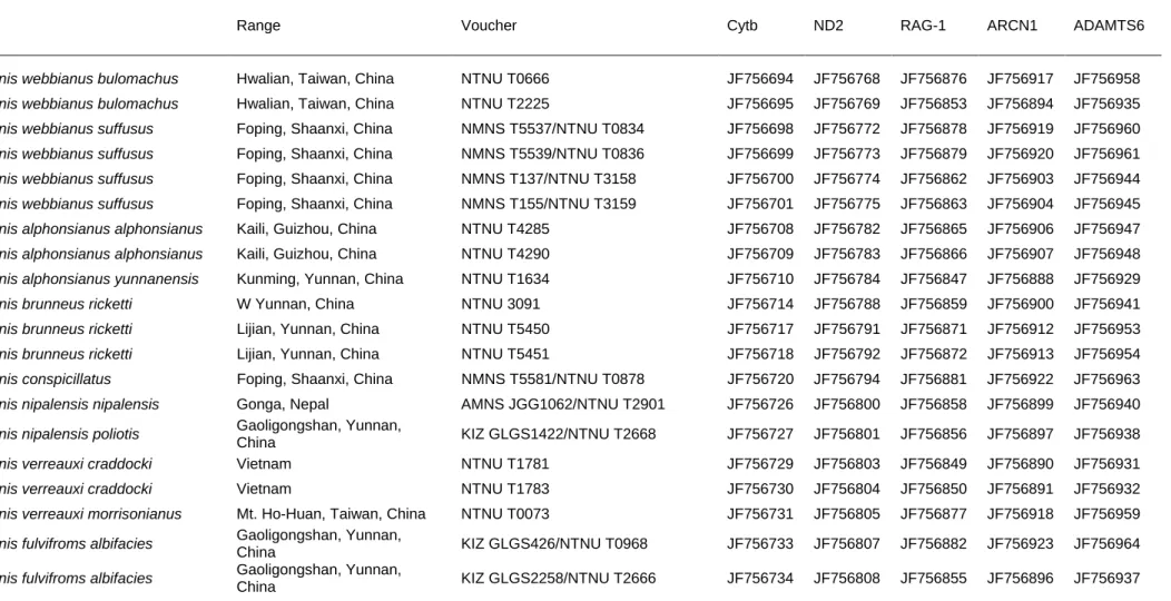
Table S1 Parrotbill species sampled and associated GenBank accession numbers for the five genes analyzed in this study.
Taxon Range Voucher Cytb ND2 RAG-1 ARCN1 ADAMTS6
Paradoxornis webbianus bulomachus Hwalian, Taiwan, China NTNU T0666 JF756694 JF756768 JF756876 JF756917 JF756958
Paradoxornis webbianus bulomachus Hwalian, Taiwan, China NTNU T2225 JF756695 JF756769 JF756853 JF756894 JF756935
Paradoxornis webbianus suffusus Foping, Shaanxi, China NMNS T5537/NTNU T0834 JF756698 JF756772 JF756878 JF756919 JF756960
Paradoxornis webbianus suffusus Foping, Shaanxi, China NMNS T5539/NTNU T0836 JF756699 JF756773 JF756879 JF756920 JF756961
Paradoxornis webbianus suffusus Foping, Shaanxi, China NMNS T137/NTNU T3158 JF756700 JF756774 JF756862 JF756903 JF756944
Paradoxornis webbianus suffusus Foping, Shaanxi, China NMNS T155/NTNU T3159 JF756701 JF756775 JF756863 JF756904 JF756945
Paradoxornis alphonsianus alphonsianus Kaili, Guizhou, China NTNU T4285 JF756708 JF756782 JF756865 JF756906 JF756947
Paradoxornis alphonsianus alphonsianus Kaili, Guizhou, China NTNU T4290 JF756709 JF756783 JF756866 JF756907 JF756948
Paradoxornis alphonsianus yunnanensis Kunming, Yunnan, China NTNU T1634 JF756710 JF756784 JF756847 JF756888 JF756929
Paradoxornis brunneus ricketti W Yunnan, China NTNU 3091 JF756714 JF756788 JF756859 JF756900 JF756941
Paradoxornis brunneus ricketti Lijian, Yunnan, China NTNU T5450 JF756717 JF756791 JF756871 JF756912 JF756953
Paradoxornis brunneus ricketti Lijian, Yunnan, China NTNU T5451 JF756718 JF756792 JF756872 JF756913 JF756954
Paradoxornis conspicillatus Foping, Shaanxi, China NMNS T5581/NTNU T0878 JF756720 JF756794 JF756881 JF756922 JF756963
Paradoxornis nipalensis nipalensis Gonga, Nepal AMNS JGG1062/NTNU T2901 JF756726 JF756800 JF756858 JF756899 JF756940
Paradoxornis nipalensis poliotis Gaoligongshan, Yunnan,
China KIZ GLGS1422/NTNU T2668 JF756727 JF756801 JF756856 JF756897 JF756938
Paradoxornis verreauxi craddocki Vietnam NTNU T1781 JF756729 JF756803 JF756849 JF756890 JF756931
Paradoxornis verreauxi craddocki Vietnam NTNU T1783 JF756730 JF756804 JF756850 JF756891 JF756932
Paradoxornis verreauxi morrisonianus Mt. Ho-Huan, Taiwan, China NTNU T0073 JF756731 JF756805 JF756877 JF756918 JF756959
Paradoxornis fulvifroms albifacies Gaoligongshan, Yunnan,
China KIZ GLGS426/NTNU T0968 JF756733 JF756807 JF756882 JF756923 JF756964
Paradoxornis fulvifroms albifacies Gaoligongshan, Yunnan,
Paradoxornis fulvifroms cyanophrys Foping, Shaanxi, China NMNS T164/NTNU T3151 JF756735 JF756809 JF756860 JF756901 JF756942
Paradoxornis fulvifroms cyanophrys Foping, Shaanxi, China NMNS T166/NTNU T3152 JF756736 JF756810 JF756861 JF756902 JF756943
Paradoxornis guttaticollis Vietnam NTNU T1797 JF756738 JF756812 JF756851 JF756892 JF756933
Paradoxornis gularis fokiensis Jinxiu, Guanxi, China KIZ DYS081/NTNU T5452 JF756744 JF756818 JF756873 JF756914 JF756955
Paradoxornis gularis fokiensis Jinxiu, Guanxi, China KIZ DYS082/NTNU T5453 JF756745 JF756819 JF756874 JF756915 JF756956
Paradoxornis gularis transfluvialis Vietnam NTNU T1816 JF756746 JF756820 JF756852 JF756893 JF756934
Paradoxornis gularis transfluvialis Quan Nam, Vietnam AMNH PRS2212/NTNU T2899 JF756747 JF756821 JF756857 JF756898 JF756939
Paradoxornis paradoxus Foping, shanxi, China NMNS T5452/NTNU T1255 JF756751 JF756825 JF756843 JF756884 JF756925
Paradoxornis paradoxus Foping, shanxi, China NMNS T5451/NTNU T1256 JF756752 JF756826 JF756844 JF756885 JF756926
Paradoxornis unicolor Yunnan, China NTNU T1683 JF756753 JF756827 JF756845 JF756889 JF756930
Paradoxornis unicolor Gaoligongshan, Yunnan,
China KIZ GLGS5058/NTNU T5108 JF756756 JF756830 JF756868 JF756909 JF756950
Paradoxornis unicolor Lushui, Yunnan, China KIZ GLGS5057/NTNU T5252 JF756757 JF756831 JF756870 JF756911 JF756952
Conostoma aemodium Foping, Shaanxi, China NMNS T38/NTNU T4512 JF756760 JF756834 JF756867 JF756908 JF756949
Conostoma aemodium Foping, Shaanxi, China NMNS T10108/NTNU T5219 JF756761 JF756835 JF756869 JF756910 JF756951
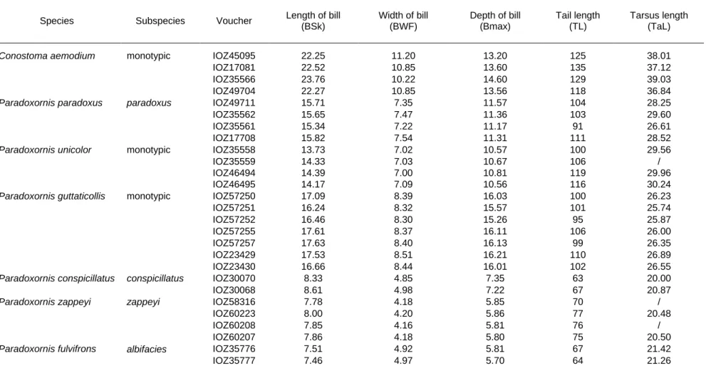
Table S2 Individuals and measurements used for morphological analyses.
Species Subspecies Voucher Length of bill (BSk) Width of bill (BWF) Depth of bill (Bmax) Tail length (TL) Tarsus length (TaL)
Conostoma aemodium monotypic IOZ45095 22.25 11.20 13.20 125 38.01
IOZ17081 22.52 10.85 13.60 135 37.12
IOZ35566 23.76 10.22 14.60 129 39.03
IOZ49704 22.27 10.85 13.56 118 36.84
Paradoxornis paradoxus paradoxus IOZ49711 15.71 7.35 11.57 104 28.25
IOZ35562 15.65 7.47 11.36 103 29.60
IOZ35561 15.34 7.22 11.17 91 26.61
IOZ17708 15.82 7.54 11.31 111 28.52
Paradoxornis unicolor monotypic IOZ35558 13.73 7.02 10.57 100 29.56
IOZ35559 14.33 7.03 10.67 106 /
IOZ46494 14.39 7.00 10.81 119 29.96
IOZ46495 14.17 7.09 10.56 116 30.24
Paradoxornis guttaticollis monotypic IOZ57250 17.09 8.39 16.03 100 26.23
IOZ57251 16.24 8.32 15.57 101 25.74 IOZ57252 16.46 8.30 15.26 95 25.87 IOZ57255 17.61 8.37 16.11 106 26.00 IOZ57257 17.63 8.40 16.13 99 26.35 IOZ23429 17.53 8.51 16.21 110 26.89 IOZ23430 16.66 8.44 16.01 102 26.55
Paradoxornis conspicillatus conspicillatus IOZ30070 8.33 4.85 7.35 63 20.00
IOZ30068 8.61 4.98 7.22 67 20.87
Paradoxornis zappeyi zappeyi IOZ58316 7.78 4.18 5.85 70 /
IOZ60223 8.00 4.20 5.86 77 20.48
IOZ60208 7.85 4.16 5.81 76 /
IOZ60207 7.86 4.18 5.80 75 20.50
Paradoxornis fulvifrons albifacies IOZ35776 7.51 4.92 5.81 67 21.42
IOZ35778 7.46 4.98 5.77 71 20.78
IOZ35779 7.76 4.94 5.89 65 21.53
cyanophrys IOZ49819 7.58 5.01 5.82 70 21.47
Paradoxornis verreauxi craddocki IOZ49868 7.11 5.42 6.88 55 16.89
IOZ49867 7.37 5.30 6.91 52 17.04 verreauxi IOZ49818 7.20 5.30 6.90 53 / IOZ44023 7.27 5.48 6.94 49 17.00 IOZ17055 7.10 5.33 6.80 49 17.37 IOZ17054 7.20 5.41 6.83 50 16.59 craddocki IOZ49869 7.28 5.41 6.87 53 16.77 KIZ019945 7.30 5.40 6.80 52 18.00 KIZ019946 7.10 5.50 6.80 53 18.00 Paradoxornis
atrosuperciliaris atrosuperciliaris IOZ58140 10.31 7.58 10.45 76 24.07
IOZ58139 10.95 7.59 10.49 86 23.54
Paradoxornis ruficeps ruficeps IOZ58141 15.63 8.16 11.12 92 28.90
IOZ58142 14.78 8.35 12.16 91 30.22
Paradoxornis gularis rasus IOZ58143 13.94 6.51 10.60 82 24.20
IOZ58144 14.33 6.65 10.76 79 25.99 IOZ58145 14.21 6.57 10.58 87 25.50 fokiensis IOZ17080 15.08 6.81 10.63 84 25.61 IOZ19514 15.13 6.75 10.75 83 25.94 IOZ23467 14.77 6.70 10.62 86 / IOZ52050 14.86 6.77 10.79 84 25.80 hainanus IOZ26152 13.95 6.57 10.20 79 25.10 IOZ26153 13.72 6.68 10.06 / / IOZ6551 14.25 6.70 9.90 / / IOZ43157 13.75 6.60 10.07 72 23.81
Paradoxornis heudei heudei IOZ23414 16.79 7.34 13.40 113 27.45
IOZ23412 16.41 7.41 13.29 105 26.21
IOZ16176 16.71 7.35 13.20 103 25.47
IOZ23427 16.60 7.38 13.22 104 /
Paradoxornis brunneus brunneus IOZ46487 8.61 4.78 7.28 58 /
IOZ46488 8.69 4.79 7.15 / 21.90
IOZ48210 8.46 4.67 7.17 65 /
IOZ48211 8.78 4.75 7.24 / 21.96
ricketti IOZ35789 8.42 4.65 7.25 65 /
IOZ35790 8.41 4.65 7.21 / /
IOZ49815 8.21 4.56 7.08 / 18.05
IOZ37955 8.75 4.66 7.10 121 18.41
Paradoxornis webbianus webbianus IOZ23444 8.92 4.76 6.19 49 /
IOZ23448 8.98 4.79 6.32 62 18.70 IOZ50430 8.79 4.70 6.15 55 18.89 IOZ50431 8.90 4.75 6.25 65 18.91 suffusus IOZ19483 8.95 4.72 6.25 56 18.94 IOZ19497 8.91 4.74 6.23 51 18.92 IOZ20789 8.97 4.73 6.28 59 18.92 IOZ20795 9.00 4.77 6.24 66 / yunnanensis IOZ32707 8.85 4.75 6.50 58 20.32 IOZ32708 8.91 4.77 6.48 53 18.87 stresemanni IOZ44013 8.88 4.74 6.96 63 18.50 IOZ44014 8.73 4.75 6.71 64 18.55 IOZ52241 8.89 4.81 6.83 55 18.59 fulvicauda IOZ6258 8.72 4.70 6.75 76 19.62 IOZ6273 8.94 4.83 6.80 66 20.54 IOZ6270 8.92 4.80 6.72 75 19.63 IOZ6297 8.99 4.83 6.83 76 /
Paradoxornis alphonsianus alphonsianus IOZ47201 8.80 4.67 6.39 60 18.85
IOZ35787 8.89 4.69 6.45 59 /
IOZ17067 8.94 4.69 6.49 58 19.24
/ 8.92 4.69 6.38 61 18.87
Paradoxornis nipalensis poliotis KIZ012944 8.10 5.20 6.60 51 18.00
KIZ012945 8.40 5.20 6.90 54 18.00 KIZ011267 8.60 5.30 7.30 55 19.00 KIZ012943 7.00 5.10 6.30 53 18.00 beaulieui KIZ008777 8.60 5.30 7.10 46 / KIZ008775 7.90 5.10 6.80 47 / KIZ020055 7.80 5.10 7.10 / / KIZ008776 8.30 5.20 7.20 / 18.00
Paradoxornis davidianus davidianus FNU2295908 10.40 5.30 8.60 36 17.10
FNU2295902 11.30 5.50 8.60 35 17.90
FNU2295903 10.90 5.50 8.50 35 17.60
FNU2295905 11.30 5.50 8.70 39 17.60
/ 11.00 5.40 8.50 39 17.70
Table S3 Different diversification models fitted to the time-calibrated species tree with parameter and support values.
λ (speciation) µ (extinction) additional parameters of diversity- and time-dependent models t (time-shift)
λ2 t2 λ3 t3 λ4 AIC ΔAIC AICc ΔAICc
1) a pure birth (Yule) 0.149 27.984 2.759 28.234 1.404
2) a rate-constant-birth-death (bd) model 0.149 0 29.984 4.759 30.784 3.954 3) yule2rate 0.145 0.644 0.184 25.225 0.000 26.939 0.109 4) yule3rate 0.242 4.997 0.854 4.798 0.073 27.255 2.030 32.255 5.425 5) yule4rate 0.242 4.997 0.854 4.798 0.052 0.644 0.184 29.604 4.379 40.804 13.974 6) DDX 0.949 x= 0.826 26.030 0.805 26.830 0.000 7) DDL 0.336 K=20.940 26.305 1.081 27.105 0.275 8) SPVAR 0.572 0.095 k=0.151 29.553 4.329 31.267 4.437 9) EXVAR 0.149 0.001 z=0.001 31.984 6.760 33.698 6.868 10) BOTHVAR 0.472 0.372 k=0.132, z=0.026 31.459 6.234 33.173 6.343
DDX, DDL: initial speciation rate
SPVAR, EXVAR, BOTHVAR: initial speciation rate, final extinction rate x= Parameter controlling the magnitude of the rate change. K=Parameter analogous to the ’carrying capacity’ parameter of population ecology
k=Parameter of the exponential change in speciation rate z=Parameter of the exponential change in extinction rate
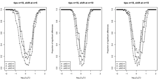
Figure S1 Proportion of cases out of 100 replicates in which a single-rate speciation model was rejected in favor of a two-rate model for trees with 18 tips. In each plot, the x-axis shows the log of the ratio between the younger rate (lambda 2) and the older rate (lambda). A ratio of zero indicates no change in rate. Results are shown for different times at which the rate shift occurred (after the appearance of 5, 10 or 15 lineages) and for different minimal AIC differences required to reject a single rate model (delta AICs of 1, 2 and 4). All simulations were performed by drawing waiting times between speciation events from an exponential distribution with rate r=l*lambda, where l is the currently extant lineages. These results suggest considerable power to detect rate shifts when changes in rate are 10-fold or more, even for "small" trees of about 18 tips.
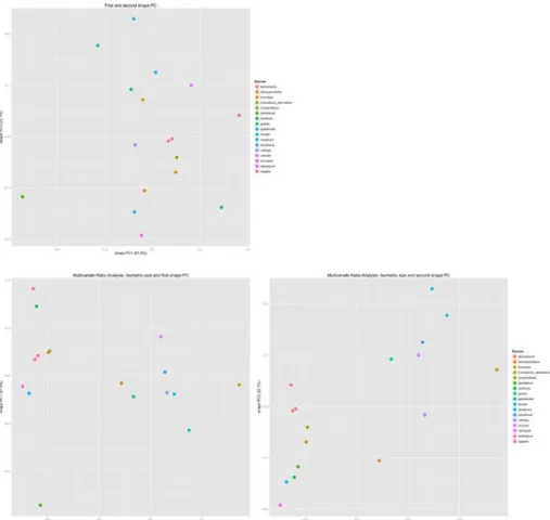
Figure S2. Scatterplot of shape PC1 against shape PC2 (top left), isosize against shape PC1 (bottom left) as well as isosize against shape PC2 bottom right.
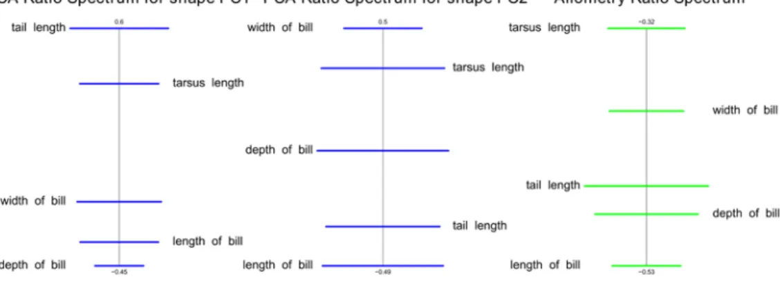
Figure S3. PCA ratio spectrum for first and second principal component in shape and allometry ratio spectrum. Ratios calculated from characters lying far apart in the ratio
spectrum explain a large part of the variance of a component, while ratios of characters lying close to each other in the spectrum contribute little to the total variance (cf. Baur &
Leuenberger, 2011). The allometry ratio spectrum is interpreted in accordance with the PCA ratio spectrum. The ratios calculated from characters lying furthest apart thus exhibit the most distinctive allometric behavior. While shape PC1 is dominated by the ratio of tail length and depth of bill length, shape PC2 is dominated by the ratio of width of bill and length of bill. The ratio that dominates shape PC1 and shape PC2 are only marginally affected by allometric relationships.
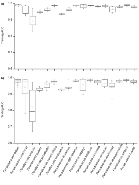
Figure S4. Discrimination ability of the Maxent model through the receiver operating characteristic curve (AUC) for parrotbill species: a) training AUC; b) testing AUC.
Figure S5. Predicted climatic suitability for parrotbill species. Values range from 1 (highest suitability) to 0 (lowest suitability).The map of distribution range in each panel (blue) represents the range limit for each species from BirdLife International and NatureServe (2014)