HAL Id: cea-01323577
https://hal-cea.archives-ouvertes.fr/cea-01323577
Submitted on 30 May 2016
HAL is a multi-disciplinary open access
archive for the deposit and dissemination of
sci-entific research documents, whether they are
pub-lished or not. The documents may come from
teaching and research institutions in France or
abroad, or from public or private research centers.
L’archive ouverte pluridisciplinaire HAL, est
destinée au dépôt et à la diffusion de documents
scientifiques de niveau recherche, publiés ou non,
émanant des établissements d’enseignement et de
recherche français ou étrangers, des laboratoires
publics ou privés.
v4, v5, v6, v7: nonlinear hydrodynamic response versus
LHC data
Li Yan, Jean-Yves Ollitrault
To cite this version:
Li Yan, Jean-Yves Ollitrault. v4, v5, v6, v7: nonlinear hydrodynamic response versus LHC data.
Physics Letters B, Elsevier, 2015, 744, pp.82-87. �10.1016/j.physletb.2015.03.040�. �cea-01323577�
Li Yan1 and Jean-Yves Ollitrault1
1
Institut de physique th´eorique, Universit´e Paris Saclay, CNRS, CEA, F-91191 Gif-sur-Yvette, France (Dated: February 10, 2015)
Higher harmonics of anisotropic flow (vnwith n ≥ 4) in heavy-ion collisions can be measured either
with respect to their own plane, or with respect to a plane constructed using lower-order harmonics. We explain how such measurements are related to event-plane correlations. We show that CMS data on v4 and v6 are compatible with ATLAS data on event-plane correlations. If one assumes
that higher harmonics are the superposition of non-linear and linear responses, then the linear and non-linear parts can be isolated under fairly general assumptions. By combining analyses of higher harmonics with analyses of v2 and v3, one can eliminate the uncertainty from initial conditions and
define quantities that only involve nonlinear hydrodynamic response coefficients. Experimental data on v4, v5 and v6 are in good agreement with hydrodynamic calculations. We argue that v7 can be
measured with respect to elliptic and triangular flow. We present predictions for v7versus centrality
in Pb-Pb collisions at the LHC.
PACS numbers: 25.75.Ld, 24.10.Nz
I. INTRODUCTION
In the last year or so, LHC and RHIC experiments have probed anisotropic flow [1] and its fluctuations [2, 3] to an unprecedented degree of precision [4–8]. These new analyses include in particular detailed analyses of higher Fourier harmonics (v4, v5, v6) and their correlations with
lower harmonics (v2, v3). The scope of this paper is
twofold. The first goal is to point out specific relations between seemingly different observables found in the re-cent experimental literature, and to propose new observ-ables. The second goal is to show that measurements of higher harmonics can be combined with measurements of lower harmonics in a way that facilitates comparison with theory. As an illustration, recent experimental re-sults are compared with hydrodynamic calculations.
The CMS Collaboration has measured v4and v6 with
respect to their own direction, and with respect to the direction of elliptic flow v2[4] (see also [8]); on the other
hand, the ATLAS Collaboration has measured a large number of event-plane correlations [5]. In Sec. II, we clarify the relation between these observables and show how they are related to one another. In particular, we show that CMS and ATLAS data on v4 and v6are
com-patible. We explain how odd harmonics, such as v5 or
v7, can also be analyzed with respect to the direction of
lower harmonics.
While recent experimental data have been compared to several theoretical models, either event-by-event hy-drodynamic calculations [9–12] or tranport models [13], these comparisons offer little insight into the physics of higher-order harmonics. In particular, theoretical calcu-lations depend strongly on the model of the initial den-sity profile, which has long been recognized as the main source of uncertainty in modeling anisotropic flow [14]. On the other hand, there are hints that the physics of higher-order harmonics should be simple: for instance, the ratio v4/(v2)2 [15, 16] is equal to 12 at high
trans-verse momentum pT in ideal hydrodynamics.
In hydrodynamics, higher-order harmonics are super-positions of linear and non-linear response terms [17–20]. This is recalled in Sec. III. We explain how the linear and nonlinear terms can be isolated under fairly gen-eral assumptions. We show how analyses of higher-order harmonics can be combined with analyses of lower-order harmonics (v2 and v3) to form quantities which do not
involve the initial state. These quantities are compared with hydrodynamic calculations.
In Sec. IV, we list a few predictions for higher-order harmonics; in particular, we predict the value of v7,
mea-sured with respect to v2 and v3, as a function of
central-ity.
II. OBSERVABLES FOR HIGHER HARMONICS Anisotropic flow is an azimuthal (ϕ) asymmetry of the single-particle distribution [21]: P (ϕ) = 1 2π +∞ X n=−∞ Vne−inϕ, (1)
where Vn = vnexp(inΨn) is the (complex) anisotropic
flow coefficient in the nth harmonic, and V−n= Vn∗. Both
the magnitude [22] and phase [2, 23] of Vnfluctuate event
to event.
The simplest observable involving Vn is a plain rms
average [24, 25]:
vn{Ψn} ≡ph|Vn|2i, (2)
where angular brackets denote an average over events. The notation vn{Ψn} has been used earlier to denote the
value analyzed with the event-plane method [4]. How-ever, the event-plane method does does not quite measure the rms average [26]. Therefore it should be replaced by the scalar-product method [27], which is recalled in Ap-pendix A. Note that our vn{Ψn} is the same quantity as
vn{2} in the notation of the cumulant analysis [28].
2 Alternatively, V4 can be analyzed with respect to the
direction of V2 [29, 30], and V6 can be analyzed with
respect to the direction of V2 or that of V3,
v4{Ψ2} ≡ RehV4(V2∗)2i ph|V2|4i v6{Ψ2} ≡ RehV6(V2∗)3i ph|V2|6i v6{Ψ3} ≡ RehV6(V3∗)2i ph|V3|4i . (3)
The triangular inequality implies |v4{Ψ2}| ≤ v4{Ψ4},
|v6{Ψ2}| ≤ v6{Ψ6}, |v6{Ψ3}| ≤ v6{Ψ6}, i.e., v4 and v6
are larger when measured with respect to their own plane than with respect to another plane. The ratio of vn{Ψm}
and vn{Ψn} (where n is a multiple of m) can be
writ-ten as the Pearson correlation coefficient between Vn and
(Vm)n/m, which we denote by ρmn: ρ24≡ RehV4(V2∗)2i ph|V4|2ih|V2|4i = v4{Ψ2} v4{Ψ4} ρ26≡ RehV6(V2∗) 3i ph|V6|2ih|V2|6i = v6{Ψ2} v6{Ψ6} ρ36≡ RehV6(V3∗)2i ph|V6|2ih|V3|4i = v6{Ψ3} v6{Ψ6} . (4)
The correlations between event planes measured by ATLAS, which are denoted by hcos(4(Φ2− Φ4))iw,
hcos(6(Φ2− Φ6))iw and hcos(6(Φ3− Φ6))iw in Ref. [5],
are precisely ρ24, ρ26 and ρ36 [13, 31]. Note that the
terminology “event-plane correlations” applied to such measurements is somewhat misleading, in the sense that these observables involve not only the angles of Vn, but
also their magnitudes [27].
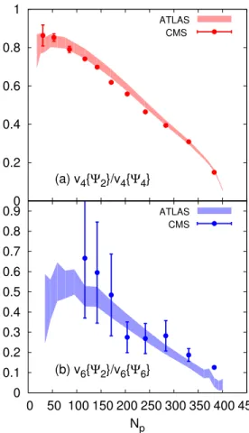
Figure 1 presents a test of the first two lines of Eq. (4), where the left-hand side uses ATLAS data and the right-hand side CMS data. The overall agreement is very good, which shows that CMS and ATLAS data are com-patible, even though they are measured with different cuts of tranverse momentum pT. Note that CMS uses
the event-plane method, instead of the scalar-product method. This method yields a slightly lower correlation when the resolution is large [5]. This explains, at least qualitatively, why CMS data are slightly lower than AT-LAS data for midcentral collisions in Fig. 1 (a).
While Pearson correlation coefficients are typically an-alyzed by integrating over all particles in a reference detector [5], analyses of vn with respect to a specific
direction (either Ψ2 or Ψn) can be done differentially,
as a function of transverse momentum pT [30] (see
Ap-pendix A for analysis details). Hydrodynamics predicts a slightly different pT dependence depending on the
refer-ence direction [18]. It is therefore interesting to general-ize Eq. (3) to odd harmonics. V5and V7can be analyzed
with respect to the directions of V2and V3 in the
follow-ing way: v5{Ψ23} ≡ RehV5V2∗V3∗i ph|V2|2|V3|2i 0 0.2 0.4 0.6 0.8 1 (a) v4{Ψ2}/v4{Ψ4} ATLAS CMS 0 0.1 0.2 0.3 0.4 0.5 0.6 0.7 0.8 0.9 0 50 100 150 200 250 300 350 400 450 Np (b) v6{Ψ2}/v6{Ψ6} ATLAS CMS
FIG. 1. (Color online) Test of Eqs. (4). Shaded bands corre-spond to the left-hand side measured by ATLAS [5] in Pb-Pb collisions at 2.76 TeV. Full circles correspond to the right-hand side, obtained using CMS data [4].
v7{Ψ23} ≡
RehV7(V2∗)2V3∗i
ph|V2|4|V3|2i
. (5)
Quantitative predictions for these quantities will be pre-sented in Sec. IV. These projected harmonics are smaller than those defined by Eq.(2), namely, |v5{Ψ23}| ≤
v5{Ψ5}, (and |v7{Ψ23}| ≤ v7{Ψ7}). The ratio of
|v5{Ψ23}| and v5{Ψ5} is again the Pearson correlation
coefficient between V5and V2V3:
ρ23,5 ≡ RehV5V2∗V3∗i ph|V2|2|V3|2ih|V5|2i =v5{Ψ23} v5{Ψ5} . (6) This quantity is very similar to the corresponding three-plane correlation measured by ATLAS [5]:
hcos(2Φ2+ 3Φ3− 5Φ5)iw≡
RehV5V2∗V3∗i
ph|V2|2ih|V3|2ih|V5|2i
. (7) More precisely, they coincide if the magnitudes of V2 and V3 are uncorrelated,1 namely, h|V2|2|V3|2i =
1 A slight anticorrelation between |V
pre-h|V2|2ih|V3|2i. Throughout this paper, we use hcos(2Φ2+
3Φ3− 5Φ5)iwfrom ATLAS as an approximation for ρ235.
Note that even though v4{Ψ2} and v6{Ψ2} are smaller
than v4{Ψ4} and v6{Ψ6}, respectively, they are measured
with better relative precision [4]. The reason is that these measurements use elliptic flow as a reference, which is measured very accurately. Triangular flow, v3, is also
precisely known. We therefore expect that v5{Ψ23} be
determined with better relative accuracy than v5{Ψ5}.
In the same way, we expect that even though no experi-ment has yet been able to detect a nonzero v7{Ψ7}, LHC
experiments could already measure v7{Ψ23}.
III. LINEAR AND NONLINEAR RESPONSE In hydrodynamics, anisotropic flow is the response to anisotropy in the initial density profile [34]. Harmonics V4 and higher can arise from initial anisotropies in the
same harmonic [3, 35–37] (linear response) or can be in-duced by lower-order harmonics [15, 38, 39] (nonlinear response). To a good approximation [20], one can write
V4= V4L+ χ4(V2)2
V5= V5L+ χ5V2V3
V6= V6L+ χ62(V2)3+ χ63(V3)2
V7= V7L+ χ7(V2)2V3, (8)
where VnLdenotes the part of Vndue to linear response,
and we have included the nonlinear terms involving the largest flow harmonics, V2 and V3. The interest of this
decomposition is that the nonlinear response coefficients χ are independent of the initial density profile in a given centrality class [18]. We now explain how the linear and nonlinear parts can be isolated.
A. Linear response
The linear part of v4 and v5 can be isolated [40] by
combining the observables introduced in Sec. II. Using Eqs. (2) and (3), one obtains
(v4{Ψ4})2− (v4{Ψ2})2= h|V4L|2i − |hV4L(V2∗)2i|2 h|V2|4i (v5{Ψ5})2− (v5{Ψ23})2= h|V5L|2i − |hV5LV2∗V3∗i|2 h|V2|2|V3|2i .(9) These results are general: these combinations always sub-tract the nonlinear response.
From now on, we further assume that the terms ap-pearing in the right-hand side of Eq. (8) are uncorrelated. That is, we neglect the small correlation between the lin-ear and nonlinlin-ear parts which is seen in Monte-Carlo
dicted in AMPT simulations [31–33], but it is at most at the 10% level.
Glauber simulations [18]. The idea behind this assump-tion is that V4L is produced by initial fluctuations in the
fourth harmonic, which are not correlated with the mean eccentricity. Then, the last term in the right-hand side of Eq. (9) vanishes, and the rms value of the linear part is v4L≡ph|V4L|2i = p (v4{Ψ4})2− (v4{Ψ2})2 v5L≡ph|V5L|2i = p (v5{Ψ5})2− (v5{Ψ23})2. (10)
This quantity has been measured as a function of cen-trality by the ATLAS collaboration [40].
B. Nonlinear response
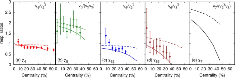
The nonlinear parts are obtained by projecting Eq. (8) onto lower harmonics. Assuming again that the terms in the right-hand side of Eq. (8) are uncorrelated, one obtains the following expressions for nonlinear response coefficients: χ4= hV4(V2∗) 2i h|V2|4i = v4{Ψ2} ph|V2|4i χ5= hV5V2∗V3∗i h|V2|2|V32|i = v5{Ψ23} ph|V2|2|V32|i χ62= hV6(V2∗)3i h|V2|6i = v6{Ψ2} ph|V2|6i χ63= hV6(V3∗) 2i h|V3|4i = v6{Ψ3} ph|V3|4i χ7= hV7(V2∗)2V3∗i h|V2|4|V32|i = v7{Ψ23} ph|V2|4|V32|i . (11) The left-hand side of these expressions can be calculated in hydrodynamics, and is independent of the model of ini-tial conditions, while the right-hand side can be inferred from experimental data. Eq. (11) therefore offers a direct comparison between hydrodynamics and data, where all dependence on initial state is eliminated [41]. Nonlin-ear response coefficients have been obtained using event-shape engineering [40] by the ATLAS collaboration. The present method does not require event-shape engineer-ing. The comparison between hydrodynamics and data is shown in Fig. 2, and we now explain in detail how these results are obtained.
The numerators in the right-hand side of Eq. (11) are the projected harmonics defined by Eqs. (3) and (5). We use v4{Ψ2} and v6{Ψ2} measured by CMS [4].2 v5{Ψ23}
and v6{Ψ3} are not measured directly, but can be
in-ferred from v5{Ψ5}, v6{Ψ6}, ρ235 and ρ36 using Eqs. (4)
and (6). We use CMS data [4] for v5{Ψ5} and v6{Ψ6}
and ATLAS data [5] for ρ235 and ρ36. These correlation
coefficients, however, are expected to depend little on the experimental setup, as illustrated in Fig. 1.
2Since CMS uses the event-plane method, the results are slightly
4 0 0.5 1 1.5 2 2.5 3 0 10 20 30 40 50 60 resp. ratios Centrality (%) v4/v22 (a) χ4 0 10 20 30 40 50 60 Centrality (%) v5/(v2v3) (b) χ5 0 10 20 30 40 50 60 Centrality (%) v6/v23 (c) χ62 0 10 20 30 40 50 60 Centrality (%) v6/v32 (d) χ63 0 10 20 30 40 50 60 Centrality (%) v7/(v22v3) (e) χ7
FIG. 2. (Color online) Nonlinear response coefficients defined by Eq. (11) as a function of centrality. Each panel corresponds to a different line of Eq. (11). Dashed lines: ideal hydrodynamics. Solid lines: viscous hydrodynamics with η/s = 0.08. Symbols: experimental data (see text for details).
The denominators in the right-hand side of Eq. (11) in-volve various even moments of the distribution of V2 and
V3. There is no direct measurement of these moments
to date. A straightforward procedure to analyze them is outlined in Ref. [31]. Alternatively, moments of the form h|Vn|2ki can be inferred from cumulants [28]. The
expressions of the first moments in terms of cumulants are:
h|Vn|2i = v2{2}2
h|Vn|4i = 2v2{2}4− v2{4}4
h|Vn|6i = 4vn{6}6− 9vn{4}4vn{2}2+ 6vn{2}6. (12)
For the moments involving both V2 and V3 (second and
fourth line of Eq. (11)), we further assume that the mag-nitudes of V2 and V3are uncorrelated.
Since different experiments have different acceptance (in particular in transverse momentum pT), it is
impor-tant to use results from the same experiment in evalu-ating the right-hand side of Eq. (11). We use cumulant results from CMS [4]. CMS has not published v2{6},
but ATLAS has observed [7] that v2{6} ' v2{4} for all
centralities, therefore we assume v2{6} = v2{4}.
The response coefficients in the left-hand side of Eq. (11) are calculated using hydrodynamics. The calcu-lation shown in Fig. 2 is the same as in Ref. [18]. It uses as initial condition a symmetric Gaussian density profile, where the normalization is adjusted to fit the measured multiplicity dNch/dy of Pb-Pb collisions at the LHC in
the corresponding centrality class. This symmetric pro-file is deformed in order to produce anisotropic flow in the desired harmonic.3 We assume uniform longitudinal
expansion [42]. With these initial conditions, we solve
3 For instance, χ
4 is obtained by introducing an elliptic
deforma-tion and calculating χ4= v4/(v2)2.
ideal hydrodynamics or second order viscous hydrody-namics [43] with constant shear viscosity over entropy ratio η/s = 0.08 [44]. The equation of state is taken from Lattice QCD [45]. The initial time of the calcula-tion is τo = 1 fm/c and the freeze-out temperature [46]
is Tf o = 150 MeV. Anisotropic flow, vn, is calculated
at freeze-out. It is averaged over particles in the inter-val pT > 0.3 GeV/c, corresponding to the CMS
accep-tance [4].
Figure 2 shows that hydrodynamics naturally captures the sign, the magnitude, and the centrality dependence of all four nonlinear response coefficients. Experimental results differ from hydrodynamic calculations only for the most central bins [41], where the linear part typically be-comes larger than the nonlinear part and their correlation can no longer be neglected.
The order of magnitude of the hydrodynamic result can be understood simply. At fixed, large pT, ideal
hy-drodynamics predicts [15, 18] χ4= 12, χ5= 1, χ62 = 16,
χ63=12, χ7=12. However, after averaging over pT, χ4is
multiplied by hv2
2i/hv2i2> 1, where brackets now denote
an average over pT in a single hydro event. This is the
reason why the results shown in Fig. 2 are larger than the fixed-pT prediction. Since v2 and v3 have similar
pT dependences, the enhancement factor is roughly the
same for all quadratic response terms: panels (a), (b), (d) show that χ5 ∼ 2χ4, χ63 ∼ χ4, in agreement with
the above values. The enhancement from averaging over pT is larger for cubic response terms than for quadratic
terms, but it is similar for both cubic terms: panels (c) and (e) show that χ7∼ 3χ62, also in agreement with the
above values.
A full hydrodynamical calculation gives results which differ somewhat from the naive predictions above. Coef-ficients from ideal hydrodynamics have a slight centrality dependence which is not captured by these formulas [47]. Viscous hydrodynamics predicts lower coefficients than
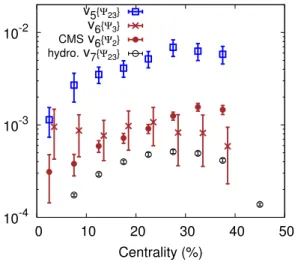
10-4 10-3 10-2 0 10 20 30 40 50 Centrality (%) v5{Ψ23} v6{Ψ3} CMS v6{Ψ2} hydro. v7{Ψ23}
FIG. 3. (Color online) v5{Ψ23}, v6{Ψ2}, v6{Ψ3} and v7{Ψ23},
averaged over charged particles with pT > 0.3 GeV/c, as a
function of centrality in Pb-Pb collisions at 2.76 TeV. v6{Ψ3}
has been shifted to the right by 1% for sake of clarity.
ideal hydrodynamics. Effect of viscosity, however, cancel to a large extent in the ratios: they are much smaller on χ4= v4/(v2)2 than on v4and (v2)2 individually [18].
Nonlinear response coefficients are mostly determined at freeze-out [18], which is probably the least understood part of hydrodynamic calculations. While they depend little on the details of the initial profile or of the hydro-dynamic evolution, they depend rather strongly on the freeze-out temperature [47]. Similarly, the dependence of our results on viscosity is mostly through the viscous cor-rection to the momentum distribution at freeze-out [48]. The momentum distribution at freeze-out is not con-strained theoretically [49, 50], and the quadratic ansatz used in this calculation is not favored by previous studies of v4 [51]. Our calculation does not involve bulk
viscos-ity, which is likely to be important at freeze-out [52–55]. Finally, our results are quite sensitive to the value of the freeze-out temperature. Further studies are needed in or-der to pin down the sensitivity of response coefficients to model parameters.
IV. PREDICTIONS
Figure 3 displays v5{Ψ23}, v6{Ψ2}, v6{Ψ3} and
v7{Ψ23}. Out of these four quantities, only v6{Ψ2} has
been measured by CMS [4]. We predict v5{Ψ23} and
v6{Ψ3} using Eqs. (4) and (6), where we take v5{Ψ5}
and v6{Ψ6} from CMS [4] and ρ235 and ρ36 from
AT-LAS [5].
Finally, v7{Ψ23} is obtained from the last line of
Eq. (11). We use the viscous hydrodynamic calcula-tion for χ7 shown in Fig. 2 (e). We again assume that
the magnitudes of V2 and V3 are independent, that is,
h|V2|4|V32|i ' h|V2|4ih|V32|i, and we estimate the moments
using Eq. (12) and CMS data [4]. We anticipate that the absolute experimental error on v7{Ψ23} should be
simi-lar to the error on v6{Ψ2}. This error is of the order of
0.01%. The predicted values of v7{Ψ23} is 0.05% in the
25-30% centrality range, larger than the error. We there-fore expect that a nontrivial v7{Ψ23} could be measured
in midcentral Pb-Pb collisions at the LHC.
V. CONCLUSION
Harmonics v4 and higher can be measured either with
respect to their own planes or with respect to lower har-monic planes. We have clarified the relation between these projected harmonics and the so-called event-plane correlations.
We have shown that under fairly general assumptions, measurements of higher harmonics can be combined with measurements of v2 and v3 in a way that eliminates the
dependence on the initial state, and can be directly com-pared with hydrodynamic calculations. Experimental re-sults for v4, v5 and v6 are in good agreement with
vis-cous hydrodynamic calculations. We have argued that v7 could be measured, and presented quantitative
pre-dictions.
On the experimental side, analyses should be repeated using the scalar-product method, whose result may differ significantly from the event-plane method for higher har-monics [27]. On the theoretical side, we hope that stud-ies of higher harmonics will help constrain the theoretical description of the fluid close the freeze-out temperature, which is poorly understood at present.
ACKNOWLEDGMENTS
LY is funded by the European Research Council under the Advanced Investigator Grant ERC-AD-267258.
Appendix A: Analysis
The flow observables in Eq. (2), (3) and (5) are ex-pressed in terms of moments of the distribution of Vn. A
generic moment is of the form [31]
M ≡ * Y n (Vn)kn(Vn∗) ln + , (A1)
where kn and ln are integers and azimuthal symmetry
implies P
nnkn = Pnnln. For instance, hV4(V2∗)2i
corresponds to k4 = 1, l2 = 2; h|V2|6i corresponds to
k2 = l2 = 3; h|V2|4|V3|2i corresponds to k2 = l2 = 2,
k3= l3= 1.
We now describe a simple procedure for measuring these moments [31], which generalizes the scalar-product
6 method [56]. We define in each collision the flow vector
by Qn ≡ 1 N X j einϕj, (A2)
where the sum runs over N particles seen in a refer-ence detector, and ϕj are their azimuthal angles. One
measures Qn in two different parts of the detector
(“subevents”) A and B, which are symmetric around midrapidity and separated by a gap in pseudorapidity in order to suppress nonflow correlations [13, 57, 58]. The moment (A1) is then given by
M = * Y n (QnA)kn(Q∗nB) ln + . (A3)
Applied to Eq. (5), this gives: v5{Ψ23} ≡
RehQ5AQ∗2BQ∗3Bi
pRehQ2AQ3AQ∗2BQ∗3Bi
. (A4)
The scalar-product method thus uses the magnitude of the flow vector [56] while the traditional event-plane method [59] only uses its azimuthal angle. One can symmetrize the numerator of Eq. (A4) over A and B to decrease the statistical error. Instead of 2 symmetric subevents, one can use 3 non-symmetric subevents, as described in Ref. [27].
Finally, analyses can be done differentially (in pT bins,
for identified particles, etc.). For the differential analysis, one replaces Eq. (A4) by:
v5{Ψ23} ≡
Rehe5iϕQ∗ 2BQ∗3Bi
pRehQ2AQ3AQ∗2BQ∗3Bi
, (A5)
where the average in the numerator is now an average over particles in the considered bin, with azimuthal angle ϕ, instead of an average over events.
[1] U. Heinz and R. Snellings, Ann. Rev. Nucl. Part. Sci. 63, 123 (2013) [arXiv:1301.2826 [nucl-th]].
[2] B. Alver et al. [PHOBOS Collaboration], Phys. Rev. Lett. 98, 242302 (2007) [nucl-ex/0610037].
[3] B. Alver and G. Roland, Phys. Rev. C 81, 054905 (2010) [Erratum-ibid. C 82, 039903 (2010)] [arXiv:1003.0194 [nucl-th]].
[4] S. Chatrchyan et al. [CMS Collaboration], Phys. Rev. C 89, no. 4, 044906 (2014) [arXiv:1310.8651 [nucl-ex]]. [5] G. Aad et al. [ATLAS Collaboration], Phys. Rev. C 90,
no. 2, 024905 (2014) [arXiv:1403.0489 [hep-ex]].
[6] B. B. Abelev et al. [ALICE Collaboration], Phys. Rev. C 90, no. 5, 054901 (2014) [arXiv:1406.2474 [nucl-ex]]. [7] G. Aad et al. [ATLAS Collaboration], Eur. Phys. J. C
74, no. 11, 3157 (2014) [arXiv:1408.4342 [hep-ex]]. [8] A. Adare et al. [PHENIX Collaboration],
arXiv:1412.1038 [nucl-ex].
[9] B. Schenke, S. Jeon and C. Gale, Phys. Rev. C 85, 024901 (2012) [arXiv:1109.6289 [hep-ph]].
[10] F. G. Gardim, F. Grassi, M. Luzum and J. Y. Ollitrault, Phys. Rev. Lett. 109, 202302 (2012) [arXiv:1203.2882 [nucl-th]].
[11] Z. Qiu and U. Heinz, Phys. Lett. B 717, 261 (2012) [arXiv:1208.1200 [nucl-th]].
[12] S. Ryu, J.-F. Paquet, C. Shen, G. S. Denicol, B. Schenke, S. Jeon and C. Gale, arXiv:1502.01675 [nucl-th]. [13] R. S. Bhalerao, J. Y. Ollitrault and S. Pal, Phys. Rev. C
88, 024909 (2013) [arXiv:1307.0980 [nucl-th]].
[14] M. Luzum and P. Romatschke, Phys. Rev. C 78, 034915 (2008) [Erratum-ibid. C 79, 039903 (2009)] [arXiv:0804.4015 [nucl-th]].
[15] N. Borghini and J. Y. Ollitrault, Phys. Lett. B 642, 227 (2006) [nucl-th/0506045].
[16] C. Lang and N. Borghini, Eur. Phys. J. C 74, 2955 (2014) [arXiv:1312.7763 [nucl-th]].
[17] F. G. Gardim, F. Grassi, M. Luzum and J. Y. Ollitrault, Phys. Rev. C 85, 024908 (2012) [arXiv:1111.6538 [nucl-th]].
[18] D. Teaney and L. Yan, Phys. Rev. C 86, 044908 (2012) [arXiv:1206.1905 [nucl-th]].
[19] D. Teaney and L. Yan, Phys. Rev. C 90, no. 2, 024902 (2014) [arXiv:1312.3689 [nucl-th]].
[20] F. G. Gardim, J. Noronha-Hostler, M. Luzum and F. Grassi, arXiv:1411.2574 [nucl-th].
[21] M. Luzum, J. Phys. G 38, 124026 (2011) [arXiv:1107.0592 [nucl-th]].
[22] M. Miller and R. Snellings, nucl-ex/0312008.
[23] R. Andrade, F. Grassi, Y. Hama, T. Kodama and O. So-colowski, Jr., Phys. Rev. Lett. 97, 202302 (2006) [nucl-th/0608067].
[24] K. Aamodt et al. [ALICE Collaboration], Phys. Rev. Lett. 107, 032301 (2011) [arXiv:1105.3865 [nucl-ex]]. [25] A. Adare et al. [PHENIX Collaboration], Phys. Rev.
Lett. 107, 252301 (2011) [arXiv:1105.3928 [nucl-ex]]. [26] B. Alver, B. B. Back, M. D. Baker, M. Ballintijn,
D. S. Barton, R. R. Betts, R. Bindel and W. Busza et al., Phys. Rev. C 77, 014906 (2008) [arXiv:0711.3724 [nucl-ex]].
[27] M. Luzum and J. Y. Ollitrault, Phys. Rev. C 87, no. 4, 044907 (2013) [arXiv:1209.2323 [nucl-ex]].
[28] N. Borghini, P. M. Dinh and J. Y. Ollitrault, Phys. Rev. C 64, 054901 (2001) [nucl-th/0105040].
[29] J. Adams et al. [STAR Collaboration], Phys. Rev. Lett. 92, 062301 (2004) [nucl-ex/0310029].
[30] A. Adare et al. [PHENIX Collaboration], Phys. Rev. Lett. 105, 062301 (2010) [arXiv:1003.5586 [nucl-ex]]. [31] R. S. Bhalerao, J. Y. Ollitrault and S. Pal, Phys. Lett. B
742, 94 (2015) [arXiv:1411.5160 [nucl-th]].
[32] P. Huo, J. Jia and S. Mohapatra, Phys. Rev. C 90, no. 2, 024910 (2014) [arXiv:1311.7091 [nucl-ex]].
[33] A. Bilandzic, C. H. Christensen, K. Gulbrandsen, A. Hansen and Y. Zhou, Phys. Rev. C 89, no. 6, 064904 (2014) [arXiv:1312.3572 [nucl-ex]].
[34] S. Floerchinger, U. A. Wiedemann, A. Beraudo, L. Del Zanna, G. Inghirami and V. Rolando, Phys. Lett. B 735, 305 (2014) [arXiv:1312.5482 [hep-ph]].
[35] D. Teaney and L. Yan, Phys. Rev. C 83, 064904 (2011) [arXiv:1010.1876 [nucl-th]].
[36] S. S. Gubser and A. Yarom, Nucl. Phys. B 846, 469 (2011) [arXiv:1012.1314 [hep-th]].
[37] Y. Hatta, J. Noronha, G. Torrieri and B. W. Xiao, Phys. Rev. D 90, no. 7, 074026 (2014) [arXiv:1407.5952 [hep-ph]].
[38] L. V. Bravina et al., Eur. Phys. J. C 74, no. 3, 2807 (2014) [arXiv:1311.7054 [nucl-th]].
[39] L. V. Bravina et al., Phys. Rev. C 89, no. 2, 024909 (2014) [arXiv:1311.0747 [hep-ph]].
[40] J. Jia, J. Phys. G 41, no. 12, 124003 (2014) [arXiv:1407.6057 [nucl-ex]].
[41] C. Gombeaud and J. Y. Ollitrault, Phys. Rev. C 81, 014901 (2010) [arXiv:0907.4664 [nucl-th]].
[42] J. D. Bjorken, Phys. Rev. D 27, 140 (1983).
[43] R. Baier, P. Romatschke, D. T. Son, A. O. Starinets and M. A. Stephanov, JHEP 0804, 100 (2008) [arXiv:0712.2451 [hep-th]].
[44] P. Kovtun, D. T. Son and A. O. Starinets, Phys. Rev. Lett. 94, 111601 (2005) [hep-th/0405231].
[45] M. Laine and Y. Schroder, Phys. Rev. D 73, 085009 (2006) [hep-ph/0603048].
[46] P. F. Kolb and U. W. Heinz, In *Hwa, R.C. (ed.) et al.:
Quark gluon plasma* 634-714 [nucl-th/0305084]. [47] M. Luzum, C. Gombeaud and J. Y. Ollitrault, Phys. Rev.
C 81, 054910 (2010) [arXiv:1004.2024 [nucl-th]]. [48] D. Teaney, Phys. Rev. C 68, 034913 (2003)
[nucl-th/0301099].
[49] K. Dusling, G. D. Moore and D. Teaney, Phys. Rev. C 81, 034907 (2010) [arXiv:0909.0754 [nucl-th]].
[50] R. S. Bhalerao, A. Jaiswal, S. Pal and V. Sreekanth, Phys. Rev. C 89, no. 5, 054903 (2014) [arXiv:1312.1864 [nucl-th]].
[51] M. Luzum and J. Y. Ollitrault, Phys. Rev. C 82, 014906 (2010) [arXiv:1004.2023 [nucl-th]].
[52] A. Monnai and T. Hirano, Phys. Rev. C 80, 054906 (2009) [arXiv:0903.4436 [nucl-th]].
[53] P. Bozek, Phys. Rev. C 81, 034909 (2010) [arXiv:0911.2397 [nucl-th]].
[54] K. Dusling and T. Schfer, Phys. Rev. C 85, 044909 (2012) [arXiv:1109.5181 [hep-ph]].
[55] J. Noronha-Hostler, G. S. Denicol, J. Noronha, R. P. G. Andrade and F. Grassi, Phys. Rev. C 88, 044916 (2013) [arXiv:1305.1981 [nucl-th]].
[56] C. Adler et al. [STAR Collaboration], Phys. Rev. C 66, 034904 (2002) [nucl-ex/0206001].
[57] S. S. Adler et al. [PHENIX Collaboration], Phys. Rev. Lett. 91, 182301 (2003) [nucl-ex/0305013].
[58] M. Luzum, Phys. Lett. B 696, 499 (2011) [arXiv:1011.5773 [nucl-th]].
[59] A. M. Poskanzer and S. A. Voloshin, Phys. Rev. C 58, 1671 (1998) [nucl-ex/9805001].