HAL Id: halshs-02794166
https://halshs.archives-ouvertes.fr/halshs-02794166
Preprint submitted on 5 Jun 2020HAL is a multi-disciplinary open access archive for the deposit and dissemination of sci-entific research documents, whether they are pub-lished or not. The documents may come from teaching and research institutions in France or abroad, or from public or private research centers.
L’archive ouverte pluridisciplinaire HAL, est destinée au dépôt et à la diffusion de documents scientifiques de niveau recherche, publiés ou non, émanant des établissements d’enseignement et de recherche français ou étrangers, des laboratoires publics ou privés.
National Accounts Series Methodology
Thomas Blanchet, Lucas Chancel
To cite this version:
World Inequality Lab Working papers n°2016/1
"National Accounts Series Methodology"
Thomas Blanchet, Lucas Chancel
Keywords : Economic inequality; National Accounts; methodology; Net national
income; gross
domestic product; net foreign income; fixed capital; inequality measurement
National Accounts Series Methodology WID.world Thomas Blanchet, PSE Lucas Chancel, PSE/Iddri This version: 22th September 2016 Overview
This methodological note presents the methodology followed to construct homogeneous series of national accounts presented on WID.world (i.e. series of net national income, gross domestic product, net foreign income, consumption of fixed capital and population) covering (almost) all countries in the world, from at least 1950 to today.
Introduction
Net national income (NNI) is a key concept to monitor the dynamics of global and domestic economic inequalities. Contrary to gross domestic product (GDP), NNI takes into account net foreign income flows and capital depreciation. Therefore, it better reflects the true evolution of individual incomes in a country and can be more easily connected to personal income. However, while it is possible to find homogenous GDP series for all countries and over a long time period on many macroeconomic data portals (such as the World Bank), there are no published global harmonized NNI series. At least two main reasons can explain this. First, despite the growing recognition that GDP is a very imperfect measure of progress (Stiglitz, Sen, & Fitoussi, 2009), GDP remains the benchmark indicator for the measure of economic growth and for the comparison of the economic performance of nations. As a result, statistical institutions invest time and resources to maintain global and consistent GDP series in priority, sometimes at the expense of other macroeconomic series. The second reason is methodological: in the United Nations Systems of National Accounts (UNSNA), NNI is a function of GDP. NNI has not always been constructed from GDP: one of the founding father of national accounting, W. Petty, constructed national income via a bottom up method, summing all incomes measured in the economy. With the development of the UNSNA, the measurement of National Income gradually became “top-down”, i.e. it is defined as a function of GDP, consumption of fixed capital (CFC) and net foreign income (NFI). In the data provided by countries to the UNSNA, CFC series are missing for several countries and time periods and sometimes indicate possibly erroneous values. It is then necessary to reconstruct robust CFC series before producing NNI series. NFI, estimates, on the other hand, can be found for a relatively large number of countries and years from the International Monetary Fund (IMF), but these series do not sum to zero at the global level — the so-called “missing income” problem (Zucman, 2013). To ensure global consistency of NFI series to a reasonable extent, reallocation rules must be developed. Such adjustments, estimations and imputations require several hypotheses and an important data cleaning work, given the need to combine different statistical sources for a large number of countries over a relatively long time frame. This note is structured as follows: we define the concepts used and detail our raw sources (1), describe the methodology followed to harmonize series (2) and the estimations performed to fill data gaps (3). We then discuss the most salient results of these new series (4) and key issues for future work (5).
1. Concept definitions, scope and data sources.
1.1 Population
In WID.world, the population of a country is defined as the de facto population of a country in the 1st of July of the year indicated. We use in priority the population data provided by the WID researchers, which usually come national demographic or fiscal institutes. Otherwise, the population series come from the United Nations World Population Prospects (WPP) (2015), providing total population, as well as population by age group and by gender, for all countries, from 1950 to 2015. In a few cases, we also use the population series published by the UNSNA in its Main Aggregates database.
1.2 Gross domestic product
Gross domestic product is defined, as in the UNSNA, as the value of final goods and services produced in a country. Here again, our priority source is the data sent by WID.world fellows, directly collected from countries’ National Accounts tables. Otherwise, we use the series from the UNSNA, the World Bank, the IMF, or Maddison (2004). The UNSNA database is divided in two parts. The Detailed Tables contains highly detailed data on GDP and its subcomponents, going back to 1946 at the earliest. It distinguishes series based on the various reviews of National Accounts System (the major UN SNA rounds are 1947, 1953, 1968, 1993 and 2008), and other secondary methodological aspects. Although rich in information, this data source provides series with many breaks. The Main Aggregates Database provides fewer series over a shorter time span (1970–2014), but covers the entire period without any breaks. The World Bank website provides GDP series, usually back to 1990, and sometimes 1960. A secondary source from the World Bank, distinct from its main data portal, is the World Bank Global Economic Monitor. It provides some of the most up to date economic data for most countries, so it can be a precious source in the most recent years. However, probably because it relies on preliminary estimates with partial coverage of the economy, it tends to give lower GDP in levels than other sources. The IMF GDP data come from its biannual publication World Economic Outlook. The database only starts in 1980, but provides forecast of GDP for the most recent years, which can be useful when no better option is available. Finally, Maddison (2004) provides data of GDP worldwide until the year 0, although we only use its post-1950 estimates. The Maddison database is used for some of the oldest GDP estimates.
1.3 Net foreign income
Net foreign income (NFI) is equal to net property income received from abroad (property income received minus property income paid) and net compensation of employees received from abroad (compensation of employees received minus compensation paid to foreign countries). Property income covers investment income from the ownership of foreign financial claims (interest, dividends, rent, etc.) and nonfinancial property income (patents, copyrights, etc.). Net foreign income is also termed as “Net primary income from abroad” in Balance of Payments tables. The raw NFI series we use come from two sources: the IMF Balance of Payments statistics and Piketty and Zucman (2013).
1.4 Consumption of fixed capital
Consumption of fixed capital is the decline, over a year, in the current value of the stock of fixed assets owned and used by a country as a result of physical deterioration, obsolescence or normal accidental damage. As in the standard UNSNA definition, our CFC definition takes into account the depreciation of tangible assets owned by producers and of fixed assets constructed to improve land. It also takes into accounts losses of fixed assets due to normal accidental damage, interest costs incurred in acquiring fixed assets as well as certain insurance premiums related to the acquisition or maintenance of fixed assets. Our definition however does not take into account the value of fixed assets destroyed by war or major natural disasters which occur only very rarely, the depletion of non-produced assets such as land, minerals or other deposits, losses due to unexpected technological developments that render existing assets obsolete over a very short time span (United Nations Statistics Division, 2009, pp. 211, C10.156). As reminded by Piketty and Zucman (2013), the risk of measurement error in CFC series is relatively high, given the various assumptions national accountants must make. (Piketty and Zucman, 2013, Data Appendix, pp. 151). Our raw consumption of fixed capital series either come from national statistical institutes (when sent by WID.world fellows) or the UNSNA. 1.5 Deflator and PPP To compare values over time we use, when available, GDP deflator series. When they are not available we use the Consumer Price Index. These come from the UNSNA, the IMF, the World Bank, Global Financial Data, National Statistical Institutes and country specific studies. To compare values over space, we use PPP indices published by the ICP.
1.6 Net national income
Net national income is equal to GDP minus CFC plus NFI. As stated above, NNI is a better measure of income than is GDP, since we correct the latter for the money that is spent to replace the depleting capital stock and the net income received from foreign countries. NNI series combines all the raw GDP, CFC and NFI sources presented above. Table 1 presents the breakdown of raw data sources used for each concept.
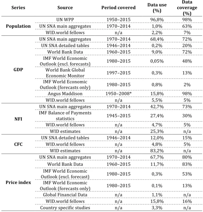
Table 1 – Coverage of raw sources used for the construction of WID.world National Accounts series
Series Source Period covered Data use (%) coverage Data (%) Population UN WPP 1950–2015 96,8% 98% UN SNA main aggregates 1970–2014 1,0% 63% WID.world fellows n/a 2,2% 7% GDP UN SNA main aggregates 1970–2014 68,4% 72% UN SNA detailed tables 1946–2014 0,2% 20% World Bank Data 1960–2015 9,0% 72% IMF World Economic Outlook (excl. forecasts) 1980–2015 0,05% 48% World Bank Global Economic Monitor 1997–2015 0,3% 13% IMF World Economic Outlook (forecasts only) 1980–2015 0,8% 2% Angus Maddison 1950–2008* 15,8% 98% WID.world fellows n/a 5,5% 5% NFI UN SNA main aggregates 1970–2014 42,7% 73% IMF Balance of Payments statistics 1945–2015 27,4% 30% WID.world fellows n/a 4,7% 5%
WID estimates n/a 25,3% n/a
CFC
UN SNA detailed tables 1946–2014 12,0% 15%
WID.world fellows n/a 4,8% 5%
WID estimates n/a 83,2% n/a
Price index UN SNA main aggregates 1970–2014 67,7% 80% World Bank Data 1960–2015 11,7% 83% IMF World Economic Outlook (excl. forecast) 1980–2015 0,3% 53% IMF World Economic Outlook (forecasts only) 1980–2015 0,1% 13%
Global Financial Data n/a 1,1% n/a
WID.world fellows n/a 15,8% 16%
Country specific studies n/a 3,3% n/a
* Maddison (2004) provides GDP data until year 0, but we only use his post-1950 estimates. Key: 12% of our CFC values come from UN SNA detailed tables and 83% of the values are reconstructed by us. UN SNA raw series cover only 15% of countries and years over the 1950-2015 period.
2. Harmonization of raw data sources
As highlighted in section 1, we use a variety of sources to reconstruct complete time series. Different series must be harmonized between sources and sometimes within each institutional source. For instance, the UN SNA tables provide, for a given concept, several series corresponding to the various reviews of National Accounts System (the major UN SNA rounds are 1947, 1953, 1968, 1993 and 2008). Each of these series often cover only a limited segment of the time period we consider. We discuss below how different series are combined with one another. 2.1 GDP The GDP series are constructed in two steps. First, we pick the GDP level in a given year and from a given source. For countries which have GDP data send by a WID.world fellow, we use that GDP level in the most recent year available. Otherwise, we use the most recent data from one of the other sources. In case of conflict, we give priority the UN SNA, then the World Bank, then the IMF. When using the UNSNA, we give priority to the Main Aggregates Database, then to the detailed tables, from the most exhaustive series to the least ones. We do not use either the IMF forecasts or the World Bank Global Economic Monitor when fixing the GDP level.
Second, we construct a continuous series of GDP growth rates. As before, we use in priority the data of the WID.world fellows, then the UN SNA, then the World Bank, then the IMF. If none of those sources has any data, which can be the case in the most recent years, we use the growth rates from the World Bank Global Economic Monitor, the IMF forecasts, or as a last resort we carry forward the growth in the last available year. All those sources typically provide data until 1970 (UN SNA), 1960 (World Bank) or 1980 (IMF). For earlier years, we use the real GDP growth rates from Maddison (2004). In China, the official GDP growth figures has been subject to criticism. Therefore, we use corrected GDP estimates from Maddison and Wu (2007). Finally, we combine the GDP growth rates with the GDP level to get a unique GDP series covering the entire time period. 2.2 Population We always give priority to the data provided by the WID.world fellows, when available, and extend those data for the most recent years using the population growth rates from the UN WPP. Otherwise, we use UN WPP estimates. We also estimate the share and the size of population groups by age and gender from the UN WPP.
There are some cases where the geographical areas of the WPP do not match the UNSNA. In France, the national accounts include the oversea territories, which are counted separately in the WPP. Also, the WPP calculates its series according to the present borders, while the UNSNA tend to provide series according to the borders of each years: that problem concerns Sudan and South Sudan, Ethiopia and Eritrea, Indonesia and East-Timor, and economies of the former Eastern Bloc. In all those cases, the UNSNA refer to larger entities than the WPP, so population series were simply aggregated to reflect the entity used in the national account series. There are other situations where the UNSNA refer to smaller entities than the WPP. In Cyprus, the WPP provides estimates for the whole Island, while the national accounts exclude the northern part. The WPP also include the Kosovo in Serbia, while they each have their own series in the UNSNA. The same problem happens with Tanzania and Zanzibar after 1990. In each of these cases, we correct the population estimates using the population series provided directly by the UNSNA. The UNSNA series, however, only provide estimates for the whole population, without any breakdown by age or gender. Hence, we assume that the population has a similar structure in the whole area and attribute to each geographical area a share of every population subcategory equal to its share of the whole population. 3. Data gaps and global (in)consistency 3.1 Consumption of Fixed Capital The UN SNA tables provide consumption of fixed capital estimates in 12% of the cases only over the 1950–2015 period1. Hence we chose to reconstruct missing UN SNA CFC estimates ourselves. To do so, we develop a statistical model that incorporate three stylized facts about CFC: • CFC tends to represent a higher fraction of GDP in more developed countries,
which can be explained by the fact that the larger the share of industrial and tertiary sector, the stronger the need to replace machinery, computer equipment, etc. • Some countries have structurally high (or low) levels of CFC. This can be due to regional or climate differences, even though regional variations did not appear to account for CFC differences in the analyses we performed. • CFC as a share of GDP is persistent: that is, if CFC is particularly high in year !, it will generally also be high in year ! + 1. This due to the fact that CFC seems to depend essentially on the structure of the economy and not on exogenous shocks. We thus model CFC as a share of GDP as a function of GDP per capita at PPP, using a log-log specification. The model includes a random effect that capture constant country characteristics. Using the index ! for the years, and $ for the countries, we have:
%&' = )*+ )+,&'+ )-,&'- + . & + /&' 1 The World Bank covers fewer years than the UN SNA (their data ranges from 1970 to 2008). WB data is itself based on several reconstructions done by WB staff, which yield odd value at times, comforting our choice to reconstruct CFC series of our own.
where %&' is the logarithm of CFC as a fraction of GDP, ,&' is the logarithm of GDP per capita at PPP, .& is the random effect term, and /&' is the error term. The square of ,&' lets us capture the concavity of the relationship between CFC and GDP per capita. We smooth the GDP using the Hodrick-Prescott filter before performing the analysis to avoid capturing short term variations of output, which would make CFC countercyclical. As in any random effect model, we assume:
0 .& ,&+, … , ,&3 = 0
To take into account the persistence of CFC, we model the error term /&' as an AR(1) process:
/&' = 5/&,'6++ 7&'
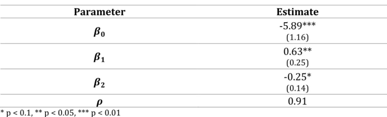
where 7&' is and i.i.d. white noise. The model can be estimated by generalized least squares using Stata’s xtregar command, which yields the following estimates: Table 2 - CFC estimation model Parameter Estimate 89 -5.89*** (1.16) 8: 0.63** (0.25) 8; -0.25* (0.14) < 0.91 * p < 0.1, ** p < 0.05, *** p < 0.01
We can check on the following autocorrelogram that /&' does exhibit persistence, but that the error term is correctly whitened once we take the AR(1) process into account:
We impute missing CFC values in the data using the model’s best prediction, using all the information at our disposal. When we know part of the CFC series, we can estimate the country’s random effect .&, so we use it in the imputation. Given the persistence of the
error term, the imputed CFC series slowly go back to their long-run expected value given the development level and fixed country characteristics, at a rate 5', without any sharp
break. When no CFC is available for any year, we simply assume .& = 0 and impute the CFC value based solely on the level of development.
3.2 Net foreign income
Net Foreign income measures net capital or labor income received by a country from nationals living abroad. While reconstructing global NFI series a problem arises: the sum of all foreign incomes does not sum to zero. This is likely due, in part, to measurement errors but also very plausibly due to the fact that a non-negligible share of global wealth is still undeclared (Zucman, 2014). This results in a significant share of global foreign income that is also undeclared. We proceed as follows, on the basis of data expressed in US dollar at market exchange rates of each year. Indeed, there is no reason why data expressed in Purchasing Power Parities should sum to zero.
Different discrepancies are observed: global foreign wage income is negative, as well as foreign investment income. However, foreign direct investment income is positive, while portfolio and other investment income is negative at the global level. While the discrepancy observed on portfolio and other investment income can be attributed to missing wealth, it is hard to explain the positive net global foreign direct investment income figures. It thus calls for different foreign income reallocation strategies, depending of the type of income reallocated.
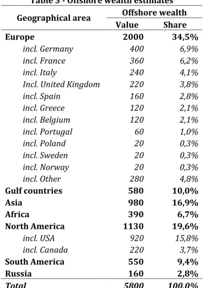
We use IMF NFI data from the Balance of Payments Statistics to compute global missing property income, i.e. the sum of all net foreign property incomes throughout the world. In the same way, we compute missing global foreign compensation income. We then allocate the global property missing income to countries or geographical regions on the basis of their share of global offshore financial wealth, based on Zucman (2014) (see table 3). Within each geographical area, we attribute missing income to countries as a fraction of their share of GDP.
Table 3 - Offshore wealth estimates Geographical area Offshore wealth Value Share Europe 2000 34,5% incl. Germany 400 6,9% incl. France 360 6,2% incl. Italy 240 4,1% Incl. United Kingdom 220 3,8% incl. Spain 160 2,8% incl. Greece 120 2,1% incl. Belgium 120 2,1% incl. Portugal 60 1,0% incl. Poland 20 0,3% incl. Sweden 20 0,3% incl. Norway 20 0,3% incl. Other 280 4,8% Gulf countries 580 10,0% Asia 980 16,9% Africa 390 6,7% North America 1130 19,6% incl. USA 920 15,8% incl. Canada 220 3,7% South America 550 9,4% Russia 160 2,8% Total 5800 100,0% Source: Zucman (2014), JEP, Data Appendix Neutral reallocation We allocate global missing (or excess) compensation of employees’ income to countries and excess Foreign Direct Investment as a function of gross domestic product shares. Global FDI excess could in fact be explained by the fact that developing countries measure FDI at their book values rather than at their market values, as suggested by Zucman (2013). Following this argument, we one could allocate excess FDI to developing countries only (i.e. increase their liabilities). However, there is no sufficient data to prove this, we thus follow a more conservative and neutral approach.
4. PPP and Price indexes
The WID.world database stores constant/real terms in “hard” (in local currency), while on the fly computations allow to move back to current/nominal values, using a national income price index (NIPI) based on GDP Deflator series when available and CPI series otherwise. We prefer the deflator as it is generally better than consumer price index (CPI) series at accounting for changes in consumer preferences over time — the so-called “substitution” bias. When such changes are not taken into account, inflation can be overestimated. GDP deflator series, in general address this issue by using chain-weighting techniques, i.e. indexes in which quantities’ weights can vary over time (Piketty and Zucman, 2013, Technical Appendix, pp. 39). On the opposite, CPI series generally use Laspeyres indexes, i.e. indexes in which quantities’ weights are fixed at the base year and which do not allow for changes in consumers’ preferences. This choice is consistent with “Capital is back” (Piketty & Zucman, 2013) (see Technical Appendix, pp. 39). In a few countries, neither official deflator nor CPI data can be found. In these cases, we use country specific case-studies. In other countries, the official inflation series have been subject to criticism: in such cases, we use alternative estimates. In particular, our inflation series for China come from Maddison and Wu (2007), and our inflation series in the recent years for Argentina come from ARKLEMS2. 4.1.1 PPP and market exchange rates WID.world stores constant local currencies and computes on the fly purchasing power parity estimates (PPP) and market exchange rates values. Our general rule for exchange rates is to preserve growth rates of series expressed in constant local currency, i.e. to convert an entire series of country A in euros at market exchange rate, we use the series stored in WID.world (expressed in constant local currency) and divide all the values by the market exchange rate between local currency and euro in the reference year (2015). We thus store only one market exchange rate value for each country and international currency. The same method is used for PPP conversions. We use the latest PPP round (ICP 2011, published in 2014). Let us remind that previous official PPP estimates (ICP 2005, published in 2008-2011) led to a significant lowering of China's, India’s and other developing countries’ GDP levels compared to previous ICP estimates. The growth rates were unchanged, but official PPP GDP series for China and India were adjusted downwards. This opened-up a controversy: Angus Maddison for instance refused to make this adjustment, arguing that the new PPP estimates lead to implausibly low per capita GDP estimates for China in 1950 (below subsistence level). See his “Background Note on Historical Statistics” (2010). In Capital in the 21st Century, Piketty uses Maddison’s estimates except for China and India which are corrected to match key international organizations estimates — the official source of economic data.
Table 4 – ICP controversy
Year 2005 ICP 2011 ICP Implied re-evaluation
India 2005 14.67 11.3 30%
China 2005 3.45 2.8 23%
The latest round (ICP 2011) re-evaluated China and India’ PPP, along with other developing countries’ PPP, and revealed that price levels were apparently too high in the 2005 round, compared what comes out from 2011 round’s methodology. One of the reason was the use, in the 2005 round, of several uncommon, expensive goods in developing countries which artificially increased the price levels in such counties — e.g. a bottle of Bordeaux. In the 2011 methodology, it was easier to avoid unrepresentative, expensive goods in the methodology used to compute price levels of developing countries. This led to the reduction in the price levels of such countries and thus in the relative strengthening of developing countries’ currencies. In WID.world, we use the 2011 PPP round and use the same extrapolation method as the World Bank to obtain 2015 PPP conversion rates: that is, we correct the 2011 PPP rate with the relative evolution of local National Income Price Index to that of the US dollar: ===-*+>?@A/ACD = ===-*++?@A/ACD EF=F-*+> EF=F-*++ EF=F-*+>AC EF=F-*++AC 5. Overview of main results Table 5A presents the distribution of 2015 global Net National Income in 2015 PPP, along with Gross Domestic Product, as well as the GDP shares of Fixed Capital Consumption and Net Foreign Incomes by world regions. Table 5B converts the values at 2015 market exchanges rates. Global GDP is of PPP€86 billion in 2015. The share of global GDP that goes into Fixed Capital Consumption is 14%. Regional CFC values range from 6% of GDP in Eastern Europe to 21% of GDP in highly industrialized Japan, showing vast disparities across region, which are further discussed below. Global Net Foreign income, measured at market exchange rate values is zero as it should be given our attempt to bridge the missing income gap (see above). When measured at PPP values global NFI comes to about -0.2% of world GDP. This is inherent to the PPPs purpose and methodology. At market values, the largest NFI surplus regions are Japan (3.9%) and North America (0.7%). Regions with lowest NFI values are Russia/Ukraine, Australia/New Zealand and Latin America (-3%, -2.4%, -2.2% respectively). Chinese and Indian NFI are zero in 2015 as there are no published data. Instead of estimating current NFI on the basis of latest available data, given the volatility of NFI, we prefer to display 0. Net National Income at the global level is 14% lower than GDP, i.e. 74 billion euros PPP (and 56 billion euros at market values). Europe and America make up exactly as much as Asia, representing 47% each of world income. European Union, North America and China also represent (almost) exactly the same share of global income: 17% each for the first two regions and 18% for China.
In terms of monthly per capita average, global per capita income is of PPP€ 845, this is also the average value in Latin America. Monthly per capita income is almost PPP€ 2000 in the European Union, about the same level as in Japan and close to PPP€ 3000 in the USA/Canada, while it is approximately PPP€ 800 in China and PPP €340 in India. The poorest region in terms of PPP is unsurprisingly Sub-Saharian Africa, with PPP€ 211 per capita per month.
Table 5A – Distribution of world National Income in 2015 (current PPP Euros)
Notes: Russia/Ukraine also includes Belarus, Albania, Bosnia, Moldova, i.e. all non E.U Eastern European countries.
Table 5B – Distribution of world National Income in 2015 (current market Euros)
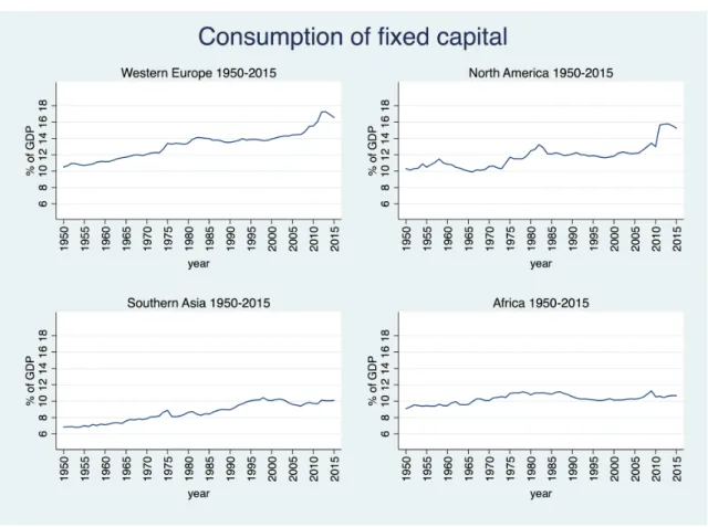
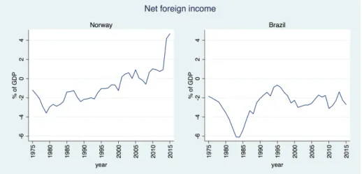
We present below CFC results for Europe, North America, Southern Asia and Africa as well as NFI results for Norway. CFC increased relatively steadily in Western Europe, rising from 11% of GDP in 1950 to more than 16% of GDP today. Consumption of Fixed Capital in North America also rose from about 10% of GDP in 1950 to about 14-15% today, even though the trend is not as steady as in Western Europe. The trajectories are notably different in Southern Asia and Africa as expected: in Southern Asia, CFC is around 7% at the beginning of the period and reaches barely 10% at the end, that is European and North American levels in the 1950s. African CFC is slightly below 10% of GDP in 1950 and slightly above 10% in 2015, showing almost no evolution in sixty-five years. Figure 2 – Regional CFC evolutions from 1950 to 2015 Source: WID.world The evolution of Norwegian NFI is illustrative of the country’s industrial trajectory and investment strategy. Following the development of oil production in the Scandinavian country in the 1990s, its negative NFI (about 3% of GDP in the 1970s) was progressively transformed into a positive NFI of about 3% of GDP today. This is due to Norwegian investments in foreign assets made possible by oil money, largely via the Norwegian Oil Fund. Brazil NFI evolution shows another story, with a large drop in the early 1980s at the time of the Brazilian economic turmoil (recession, high inflation, foreign debt crisis). These two examples indeed confirm the importance to take into account Net Foreign Incomes when comparing macro economic or individual incomes over time and countries.
Figure 3 – NFI evolution from 1975 to 2015 in Norway and Brazil Source: WID.world 6. Discussion Our data contains Net National Income, GDP, CFC and NFI series for all countries in the world from 1950 to today. We tried to harmonize the data as much as possible but several limitations indeed remain. One key issue relates to PPP estimates: our methodology assumes that the modification of production and consumption structures in two countries are well taken into account by the evolution of relative national income price indices. There are indeed strong arguments suggesting that this is an over simplification (McCarthy, 2011). We could use instead previous ICP rounds to readjust PPP values on the ICP survey years, as it is done in the Penn World Tables. More precisely, instead of assuming that Australia national income in 1970 expressed in 2015 PPP euros is a function of 2011 European and Australian production and consumption structures and price levels (as measured by the latest ICP round), and of the relative evolution of national income price indices between 1970 and today, we could use the 1980 ICP round to get closer to the “true” PPP correspondence between Australian Dollars and Euros in 1970. Given that there are few countries with relevant PPP data before 2005, this would not change the results in older time periods. However, it would give a lot of importance to variations in hard-to-measure purchasing power parities in the assessment of a country’s growth performance in recent years (see for example the ICP controversy for China and India in section 4.1.1). We thus preferred to rely solely on the most recent ICP round, and use the evolution of the price index to extrapolate in previous years.
Another issue relates to the treatment of ex-USSR countries during the soviet period. From 1950 to 1991, we only have national accounts data for USSR as a block, except for one single year, 1973, for which Maddison provides GDP values for USSR countries. This allows us to plot ex-USSR countries national income series from 1973 onwards, but we did not reconstruct national level series before this date. In order to derive robust estimates at the national level before 1973, a much closer focus on national economic and social histories is required.
Bibliography Maddison, A. (2004). The World Economy: Historical Statistics. OECD Development Centre. Maddison, A. (2010, 3). Background Note on “Historical Statistics”. Maddison, A., & Wu, H. (2007). China's Economic Performance: How Fast Has GDP Grown; How Big is it Compared to the USA? Piketty, T., & Zucman, G. (2013). Capital is Back: Wealth-Income Ratios in Rich Countries 1700-2010. 129(3), 1155-1210. Stiglitz, J. E., Sen, A., & Fitoussi, J.-P. (2009). Commission on the Measurement of Economic Performance and Social Progress. Paris: INSEE. United Nations Statistics Division. (2009). System of National Accounts 2008. New York: United Nations. United Nations, Department of Economic and Social Affairs, Population Division. (2015). World Population Prospects: The 2015 Revision, Methodology of the United Nations Population Estimates and Projections. New York: United Nations. Zucman, G. (2013). The Missing Wealth of Nations: Are Europe and the U.S. net Debtors or net Creditors? The Quarterly Journal of Economics, 128(3), 1321-1364. Zucman, G. (2014, Fall). Taxing across Borders: Tracking Personal Wealth and Corporate Profits. Journal of Economic Perspectives, 28(4), 121-48.