The potential of a constellation of low earth orbit satellite imagers to monitor worldwide fossil fuel CO2emissions from large cities and point sources

HAL Id: hal-03032332

https://hal.archives-ouvertes.fr/hal-03032332

Submitted on 26 Jan 2021

HAL is a multi-disciplinary open access

archive for the deposit and dissemination of

sci-entific research documents, whether they are

pub-lished or not. The documents may come from

teaching and research institutions in France or

abroad, or from public or private research centers.

L’archive ouverte pluridisciplinaire HAL, est

destinée au dépôt et à la diffusion de documents

scientifiques de niveau recherche, publiés ou non,

émanant des établissements d’enseignement et de

recherche français ou étrangers, des laboratoires

publics ou privés.

CO2emissions from large cities and point sources

Franck Lespinas, Yilong Wang, Grégoire Broquet, François Marie Bréon,

Michael Buchwitz, Maximilian Reuter, Yasjka J. Meijer, Armin Loescher,

Greet G.A. Janssens-Maenhout, Bo Zheng, et al.

To cite this version:

Franck Lespinas, Yilong Wang, Grégoire Broquet, François Marie Bréon, Michael Buchwitz, et al..

The potential of a constellation of low earth orbit satellite imagers to monitor worldwide fossil fuel

CO2emissions from large cities and point sources. Carbon Balance and Management, BioMed Central,

2020, 15 (1), �10.1186/s13021-020-00153-4�. �hal-03032332�

RESEARCH

The potential of a constellation of low earth

orbit satellite imagers to monitor worldwide

fossil fuel CO

₂

emissions from large cities

and point sources

Franck Lespinas

_{, Yilong Wang}

_{, Grégoire Broquet}

_{, François‑Marie Bréon}

_{, Michael Buchwitz}

_,

Maximilian Reuter

_{, Yasjka Meijer}

_{, Armin Loescher}

_{, Greet Janssens‑Maenhout}

_{, Bo Zheng}

_{and Philippe Ciais}

Abstract

Background: Satellite imagery will offer unparalleled global spatial coverage at high‑resolution for long term

cost‑effective monitoring of CO₂ concentration plumes generated by emission hotspots. CO₂ emissions can then be estimated from the magnitude of these plumes. In this paper, we assimilate pseudo‑observations in a global atmos‑ pheric inversion system to assess the performance of a constellation of one to four sun‑synchronous low‑Earth orbit (LEO) imagers to monitor anthropogenic CO₂ emissions. The constellation of imagers follows the specifications from the European Spatial Agency (ESA) for the Copernicus Anthropogenic Carbon Dioxide Monitoring (CO2M) concept for a future operational mission dedicated to the monitoring of anthropogenic CO₂ emissions. This study assesses the uncertainties in the inversion estimates of emissions (“posterior uncertainties”).

Results: The posterior uncertainties of emissions for individual cities and power plants are estimated for the 3 h

before satellite overpasses, and extrapolated at annual scale assuming temporal auto‑correlations in the uncertain‑ ties in the emission products that are used as a prior knowledge on the emissions by the Bayesian framework of the inversion. The results indicate that (i) the number of satellites has a proportional impact on the number of 3 h time windows for which emissions are constrained to better than 20%, but it has a small impact on the posterior uncertain‑ ties in annual emissions; (ii) having one satellite with wide swath would provide full images of the XCO2 plumes, and is

more beneficial than having two satellites with half the width of reference swath; and (iii) an increase in the precision of XCO2 retrievals from 0.7 ppm to 0.35 ppm has a marginal impact on the emission monitoring performance.

Conclusions: For all constellation configurations, only the cities and power plants with an annual emission higher

than 0.5 MtC per year can have at least one 8:30–11:30 time window during one year when the emissions can be constrained to better than 20%. The potential of satellite imagers to constrain annual emissions not only depend on the design of the imagers, but also strongly depend on the temporal error structure in the prior uncertainties, which is needed to be objectively assessed in the bottom‑up emission maps.

Keywords: Satellite imager, PMIF global inversion system, Anthropogenic CO₂ emissions, Posterior uncertainty

© The Author(s) 2020. This article is licensed under a Creative Commons Attribution 4.0 International License, which permits use, sharing, adaptation, distribution and reproduction in any medium or format, as long as you give appropriate credit to the original author(s) and the source, provide a link to the Creative Commons licence, and indicate if changes were made. The images or other third party material in this article are included in the article’s Creative Commons licence, unless indicated otherwise in a credit line to the material. If material is not included in the article’s Creative Commons licence and your intended use is not permitted by statutory regulation or exceeds the permitted use, you will need to obtain permission directly from the copyright holder. To view a copy of this licence, visit http://creat iveco mmons .org/licen ses/by/4.0/. The Creative Commons Public Domain Dedication waiver (http://creat iveco mmons .org/publi cdoma in/ zero/1.0/) applies to the data made available in this article, unless otherwise stated in a credit line to the data.

Background

Cities, thermal power plants and industrial sites are the largest emitters of fossil fuel CO2 that causes global

warming [10]. Monitoring CO2 emissions from these

hot-spots is therefore a priority for assessing the effectiveness

Open Access

*Correspondence: wangyil@igsnrr.ac.cn

1 _{Laboratoire des Sciences du Climat et de L’Environnement, CEA‑CNRS,}

UVSQ‑Université Paris Saclay, Gif‑sur‑Yvette, France

of greenhouse gas (GHG) emissions reduction policies. Knowledge of the magnitude and spatial and temporal variability of CO2 emissions at the regional scale is also

critical in unraveling the natural sources and sinks of the carbon cycle. Existing inventories of CO2 emissions from

fossil fuel combustion can provide accurate information at the national and annual scales in the most developed countries, but they are subject to many uncertainties in developing countries and at the scale of cities, individual point sources (e.g. power plants) and regions due to a lack of local statistical data on energy and fuel

consump-tion [1, 13]. Furthermore, regulations and commitments

are taken at the scale of cities and individual sectors. It is thus necessary to develop systems capable of providing

frequent and accurate estimates of CO2 emissions at the

scale of anthropogenic emission hotspots.

The method for monitoring anthropogenic CO2

emis-sions from these hotspots, called atmospheric inversion,

combines prior information on local CO2 emissions from

inventories with observations of atmospheric CO2

con-centrations sensitive to emissions, using atmospheric transport models and statistical inversion (e.g.[5, 17]).

The underlying idea is that CO2 concentration

meas-urements can be used to characterize downwind CO2

plumes from large emission hotspots. Dense observa-tions of the CO2 mole fractions in the atmosphere

facili-tate the characterization of CO2 emission plumes that

is used to retrieve emission estimates. In  situ

measure-ments of CO2 mole fractions from surface networks,

air-craft campaigns and mobile platforms have been used to

quantify the emissions from cities and power plants [5,

17, 30–32]. However, such networks are deployed for few cities and point sources only. The cost for maintaining a given urban network of to conduct regular campaigns around a given source limits for their deployment. Fur-thermore, the atmospheric inversions can be hampered by the discrete and limited spatial (both horizontally and vertically) sampling of fixed networks [30] or by the lack of temporal representativeness of the infrequent mobile campaigns. Alternatively, vertically integrated columns of dry-air mole fractions of CO2 (XCO2) from satellites

offer the advantage of providing full spatial coverage of the plumes of individual sources and covering a wide range of sources over the world, in cloudless conditions.

For example, Nassar et al. [22] used the XCO2

observa-tions from OCO-2 to quantify CO2 emissions from seven

middle- to large-sized coal power plants from USA, India

and South Africa. Wu et  al. [37] estimated CO2

emis-sions from 20 cities across several continents using the

XCO2 observations from OCO-2. Zheng et al. [38]

devel-oped an algorithm for the automatic detection of plumes

and inversion of fossil fuel CO2 emissions in the OCO-2

XCO2 data applied it to estimate the emissions from 46

cities and power plants in China using 5 years of OCO-2 data. These studies and some others (e.g. [14, 29]) reveal

that a limited amount of clear transects of XCO2 plumes

from cities or plants are currently detected in OCO-2 observations so that the real data from current on-orbit satellites keep on being hardly used to estimate anthro-pogenic CO2 emissions.

. In this context, there is growing interest in develop-ing satellite imager instruments capable of providdevelop-ing high spatial resolution measurements of vertically integrated columns of dry air mole fractions of CO2 (XCO2) over

the globe (e.g.[4, 8]). In particular, the European Spatial Agency (ESA) is studying the potential of the Coperni-cus Anthropogenic Carbon Dioxide Monitoring (CO2M)

mission consisting of a constellation of CO2 imagers to

monitor anthropogenic CO2 emissions.

Many studies were conducted to assess the potential of satellite imagery to reduce uncertainties in fossil CO2

emissions at the regional (e.g. [23]). and city (e.g. [6]). scales, and for point sources (e.g.[4, 15, 27, 34]). These studies showed that satellite images must have a high

spa-tial resolution between 1–20 km2 _{to accurately monitor}

CO2 plumes from cities and point sources with sufficient

cloudless observations (e.g.[4]). They also indicated that

a high retrieval precision (less than 1  ppm) of XCO2 is

required to quantify the enhancement of the CO2 column

in the plumes relative to the background even for large cities like Paris and Berlin [6, 25]. Among the important factors associated with the mission specifications, the swath width of the satellites was also shown to have to be larger than 100  km to frequently sample plumes of anthropogenic CO2 emissions with only a few satellites.

Based on these preliminary results, CO2M satellites were considered to follow a late morning orbit (Equator-cross-ing time at ~ 11:30, local time descend(Equator-cross-ing node) when there are, on average, fewer clouds, lower wind speeds,

and higher anthropogenic CO2 emissions than in early

afternoon [12]. The most likely option for the width of

the CO2M instrument is 300 km, but a range of options from 150 to 400 km is also being discussed.

However, most of the existing studies have focused on specific, and generally very large cities and plants and do not provide a global picture of the ability of

sat-ellite imagery to constrain CO2 emissions across a full

range of emission hotspots (with various emission rates and areas, and distances to other emission hotspots).

In this context, Wang et al. [35] presented the

“Plume-Monitoring Inversion Framework” (PMIF) global inver-sion system to assess the potential of satellite imagery

to monitor CO2 emissions from all emission hotspots

(including cities and power plants, which are called “clumps” following the global classification of such

around the globe and during a full year. The definition

of 11,314 clumps from the CO2 emission map Open

Source Data Inventory of Anthropogenic CO2 (ODIAC)

with a 1-km × 1-km spatial resolution was described in Wang et al. [36]. They represent all the CO2 sources that

can generate an XCO2 enhancement of at least 0.5 ppm

under optimistic meteorological conditions without

wind. In ODIAC, the sum of fossil fuel CO2 emissions

from all clumps of the globe account for about 72% of the global total. The PMIF inversion system is based on a Bayesian statistical framework, a global high-res-olution emission map, a global dataset on wind fields, a realistic sampling of satellite data, as well as errors on

individual XCO2 retrievals. The Bayesian framework

corrects a prior estimate of the control variables (here emission budgets for individual cities or power plants) from inventories, based on the atmospheric data, to derive a posterior estimate. The system assesses the uncertainties in the posterior estimate ("the posterior uncertainties”), which is a function of the uncertain-ties in the prior estimate (“the prior uncertainuncertain-ties”), of the observation sampling and errors and of the atmos-pheric transport. The design of the PMIF inversion system relies on a complex combination of short and regional assimilation windows and on some simplifi-cations compared to traditional inversion systems for a given assimilation window. This is necessary to limit the computational costs because of the large number of assimilated observations and the large number of con-trol variables when covering the globe and a full year. Among the most critical simplifications of PMIF is the

choice of the transport model: the CO2 plumes emitted

by the CO2 sources are modeled using a simple

Gauss-ian plume model that only takes into account the local mean wind field and the mean emissions, both over the three hours (i.e. 8:30–11:30 for CO2M mission) before the satellite overpass (~ 11:30LT). The Gaussian plume model can often hardly fit with actual plumes over long distances (due to variations in the wind field, topography, vertical mixing etc.) but is shown, when driven with suitable parameters, to provide a satisfac-tory simulation of the plume extent and amplitudes, which appear to be the main drivers of the targeted computations of uncertainties in the emissions in our

OSSE framework [35]. The choice of focusing on the

three hours before the satellite overpasses is driven by the analysis of Broquet et al. [6] indicating that the temporal representativeness of the detectable part of the plumes from a large city like Paris is about few hours when using a satellite imaging concept similar to CO2M. In addition, PMIF ignores uncertainties in the

natural fluxes and in diffuse anthropogenic emissions outside the clumps.

Wang et al. [35] used PMIF to assess the performance

of a single satellite imager for monitoring CO2

emis-sions for the full range of clumps and meteorologi-cal conditions representative of the whole globe and a full year. They found that only the clumps with annual emission budgets higher than 2 MtC per year can potentially have their emissions between 8:30 and 11:30 constrained with a posterior uncertainty less than 20% for more than 10 overpasses within the year (ignor-ing the temporal correlations in the prior uncertainty). They also aggregated the posterior uncertainties in time to investigate the potential of satellite observations to constrain daily and annual emissions. Their results revealed that the hypotheses on the temporal correla-tions of prior uncertainties have a critical impact on the potential of one satellite imager to constrain daily and annual emissions for individual clumps. Typically, annual budgets for cities with an annual budget larger

than 10MtC yr−1 _{can be constrained to less than 15%}

[35] with a strong temporal auto-correlation (prior

uncertainties in hourly emissions being fully correlated within the day and the auto-correlation between the same hours from different days being described by an exponential decaying function with 20-day correlation length), against 25% with a moderate temporal auto-correlation (with a 7-day auto-correlation length for day-to-day auto-correlation and a 12-h correlation length for hour-to-hour auto-correlations). Here, we extend the analysis of the inversion performances to cover the most likely scenarios for the CO2M mission, with a constellation of one to four LEO imagers. The other goal of the paper is to investigate the impacts of the major parameters of the instrument in CO2M mission, in order to support the optimization of its design: the

width of the swath and the precision of a single XCO2

retrieval. The metrics used are the posterior uncer-tainty in the 3 h (8:30–11:30) mean emissions and in the annual budget. This assessment is detailed for groups of clumps gathered as a function of their annual emission budgets and across all regions of the world.

The manuscript is organized as follows: Sect. 2 briefly reminds the principles, data and practical implementa-tion of the inversion system developed by Wang et al.

[35]. Section  3 presents an assessment of the

perfor-mance of inversions with the assimilation of satellite data from one to four imagers and different options

regarding the instrument swath and precision of XCO2

retrievals. Section  4 discusses the factors that may explain the variability of the results found on the inver-sions and some limitations of the inversion system.

Methods

The PMIF follows the traditional Bayesian statistical framework of the atmospheric inversions, updating a prior statistical estimates (xb_{) of a set of control variables}

x that corresponds to emission budgets for the clumps.

The update relies on the observations yo_{, on an}

observa-tion operator x → y = Mx + yfixed _{that links the control}

space and the observation space, and on the statistics of the so-called “observation error”. Here, yfixed _{is the}

signa-ture in the observation space of the CO2 fluxes that are

not controlled by the inversion. Since we ignore uncer-tainties in these fluxes, this term has no impact in the inversion computations and is ignored hereafter (and we call M the observation operator in the following). The observation error is a combination of all sources of errors in the observation operator and in the observations themselves, i.e. all source of misfits between the modeled and observed concentration other than errors in the prior estimate of the control variables. The prior uncertainties and the observation errors are assumed to be unbiased and to follow the Gaussian distributions N(0, B) and N(0,

R), where B and R represent the error covariance

matri-ces for the prior uncertainties and observation errors. The statistical estimate of the control variable updated in the Bayesian framework, called the posterior estimate, follows a Gaussian distribution N(xa_{, A), with x}a _being

the mean and A being the posterior uncertainty covari-ance matrix. The solution of the inversion is derived by:

The PMIF system is described in detail in Wang et al.

[35]. Here we only summarize the main elements.

PMIF solves for a scaling factor for the 3-h mean emis-sions between 8:30 and 11:30 and a scaling factor for the emissions during the rest time of the day (0:00–8:30 plus 11:30–24:00) for each day over 1 year and for all the clumps over the globe. The observation operator is null for the emissions between 0:00–8:30 plus 11:30–24:00 since we assume these emissions does not raise any

sig-nificant XCO2 signal in the CO2M satellite images at

11:30. The part of the observation operator M corre-sponding to emissions between 8:30 and 11:30 has two

components. The first one (Minventory) describes the

spa-tial distribution of emissions within the area of a clump and the temporal variation of the emissions within the

time window: x → E = Minventoryx. In PMIF, the spatial

distribution of the emissions are based on the Open

Source Data Inventory of Anthropogenic CO2 Emission

[24] for the year 2016, and the temporal variation of the

(1) A =  B−1_{+ M}T R−1M ₋₁ (2) xa= xb+ AMTR−1  yo−Mxb−yfixed 

emissions are derived from the monthly profile from ODIAC and the weekly and diurnal (at hourly resolution) profiles from the Temporal Improvements for Modeling

Emissions by Scaling (TIMES) product [20]. The second

component of M (Mplume) simulates the plumes of XCO2

enhancement above the background downwind given clumps: E → y = MplumeE. Mplume is the aggregation of the

XCO2 enhancement generated by each emitting pixel of

the ODIAC map within a given clump. For each emitting

pixel, we assume that the plume of XCO2 enhancement

downwind has a Gaussian shape:

where y is the XCO2 enhancement (in ppm) at a

down-wind location (i, j). The i-direction is parallel to the local mean wind direction and the j-direction is perpendicu-lar to that direction. In this study, the wind field is taken from the Cross-Calibrated Multi-Platform (CCMP)

gridded surface wind product for the year 2008 [3]. The

CCMP product consists in 6-hourly gridded wind vec-tors at a horizontal resolution of 0.25 degree. It is based on the combination of Version-7 RSS radiometer, Quik-SCAT and AQuik-SCAT scatterometer and moored buoy wind data with ERA-Interim model wind fields. σj is a function

of downwind distance i, similar to that used by Ars et al.

[2]. α is a coefficient that converts the computed CO2

enhancement (in g/m2_{) in the XCO}

2 unit of ppm,

assum-ing a standard surface pressure of 1013 hPa and a stand-ard molar mass of dry air of 28.97 g mol−1_.

In PMIF, we use the AMS (Annual component and Moderately correlated Sub-annual component) configu-ration of the prior uncertainty in the emission budgets,

as described in Wang et  al. [35], because it has a

plau-sible configuration on the temporal auto-correlation in prior uncertainties according to the comparison between inventories and actual emission proxies [16, 35]. In prac-tice, it assumes that the prior uncertainty in the emis-sions for each clump has two components. The first one is an annual component that is fully auto-correlated in time over 1 year (i.e. a bias in time), whose amplitude follows an unbiased Gaussian distribution ~ N(0, 29%). This com-ponent of the prior uncertainty accounts for unknown information about the city or point source that does not change over time. The second one is a sub-annual uncertainty component bearing some temporal auto-correlations. The temporal auto-correlation between this component of the uncertainties in hourly emissions at two instants distant by Δd days and Δh hours is formu-lated as r = exp(-Δh/τ1) × exp(-Δd/τ2), where τ1 = 12  h

and τ2 = 7d. This component of the prior uncertainty

fol-lows the distribution ~ N(0, 49%) for the 3  h emissions

(3) yi, j = α√ E 2π σ_jue −j 2 2σ_j2

between 8:30 and 11:30 and ~ N(0, 38%) for the rest 21 h emissions of the day. This second component (variable) is for emission variations that are not accounted for in the prior information of emissions, such as those linked to weather systems (heating) or specific variable activities. The total uncertainty of emissions for each control vari-able is the square root of the quadratic sum of the two uncertainty components.

PMIF assimilates satellite pseudo-observations cor-responding to the simulation of a one-year global sam-pling (using data corresponding to the year 2008) by sun-synchronous LEO satellites of the CO2M mission. The orbit has a repeat cycle of 16 days with an

Equator-crossing time of 11:30. As Eq. (1) shows that the

poste-rior uncertainty only depends on pposte-rior and observation error covariance matrices, on the observation operator, and implicitly on the structure of the observation vec-tor (i.e., on the time, location and representation of the observations through M), we only consider the preci-sion and sampling (time, location and spatial resolution) of the synthetic satellite observations. The precision

of individual XCO2 retrievals from the crude radiance

measurements (called the random measurement error) is simulated following the same formulation as in Buchwitz et al. [7] to simulate the impact of changes in the surface and atmospheric conditions, but with updated param-eters to model the impact of SNR and other instrumen-tal specifications for CO2M missions. For the reference CO2M configuration, the random measurement error is 0.7  ppm for vegetation albedo and solar zenith angle (SZA) 50º. The width of the swath in the reference con-figuration is 300 km and the horizontal resolution of the CO2M instruments is 2 km × 2 km. Various options for the random measurement error and swath width are also being considered (detailed below). The Moderate Resolu-tion Imaging Spectroradiometer (MODIS) Terra MOD35

cloud and aerosol data product (https ://modis -atmos

.gsfc.nasa.gov/MOD35 _L2/) was used to simulate cloud/ aerosol-contaminated XCO2 retrievals (see [7] for more

details). Only “good” XCO2 data that are cloud-free and

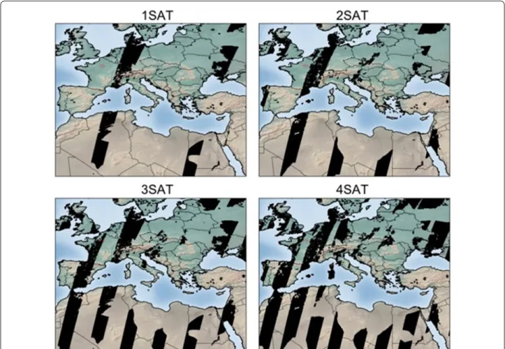
for which the sum of the retrieved aerosol optical depth (AOD) at NIR wavelength and atmosphere cirrus optical depth (COD) is less than 0.3, are used in the inversions. These data are referred to as “clear sky” data hereafter. The presence of clouds and aerosol induce data gaps in the simulated XCO2 fields (Fig. 1).

In this study, we simulate the sampling of XCO2

obser-vations from constellations consisting of one to four

CO2M imagers. The spatial coverage of the XCO2

obser-vations from the constellations are shown in Fig. 1. The

simulations for these constellations are based on com-binations of the simulations for one to four satellites on the same helio-synchronous orbit, satellites being equally

spaced in the orbit for a given constellation (Additional file 1: Fig. S1). The constellation of 3 satellites includes the satellite that is used to test the 1-satellite configuration of CO2M. Similarly, the two imagers in 2-satellite case are included in the 4-satellite constellation (Additional file 1: Fig. S1). But the 3-satellite constellation and the 4-satel-lite constellation do not have any satel4-satel-lite in common.

We conduct two sets of observing system simula-tion experiments (OSSEs) to investigate the potential of satellite observations in constraining the emissions at various time scales. The potential of satellite imagery is assessed in terms of the posterior uncertainty in the emission budgets for each clump. Firstly, we conduct an OSSE for each 8:30–11:30 window of the year seperately (called INV-3 h hereafter), ignoring the potential to cross or extrapolate the information between days based on the temporal auto-correlation in the prior uncertainty. In practice, this is done by ignoring the temporal covari-ances (off-diagonal entries) in the B matrix. The 3 h mean emissions are considered as significantly constrained when the posterior uncertainty is less than 20%. Physi-cally, it means there are at least one satellite overpass in the vicinity of the clumps and a sufficient number of

XCO2 observations with adequate precision within the

XCO2 plumes generated from the clumps. The number

of 8:30–11:30 windows for which the mean emissions are significantly constrained is denoted as N20 for each clump. Then we conduct a second set of OSSEs, in which the system fully exploits the temporal auto-correlations in B to cross information from different overpasses, and

extrapolate it to constrain emissions whose XCO2

sig-nature is not observed (that for the other 21 h within a day and the days with no satellite observations near the clump). We analyze the posterior uncertainty for the 3 h (8:30–11:30) mean emissions on all days over one year, and also for annual budget by aggregating the posterior uncertainty covariance matrix A in the second set of OSSEs. This set of OSSEs are referred to as INV-annual.

In addition to the number of satellites, the swath

width and random errors of XCO2 observations may

impact the inversion performance while some options are still under discussion for CO2M. While the refer-ence computations with the 1 to 4 satellite constel-lation are led with swath with 300  km width, and the default simulation of the random measurement error for CO2M, we change these parameters in the configu-ration of the imagers and quantify their impacts. First, we use the first and third satellites from the 4-satellite constellation and reduce the swath width of these sat-ellites to 150 km. The results are compared with those obtained with one satellite and a swath width of 300 km. Then, we reduce the random measurement error in the 3-satellite constellation (with a default swath width

of 300 km) by 20% or 50%, respectively, to investigate the benefit of improving the measurement precision in constraining the emissions. We also increase the ran-dom measurement error by 43% and 71%, such that the resulting random measurement errors are comparable

to the typical precision of XCO2 achieved by OCO-2

or simulated for GeoCARB [11],https ://cdn.event

sforc e.net/files /ef-xnn67 yq56y lu/websi te/9/739_berri en_moore _-_geost ation ary_carbo n_cycle _obser vator y__geoca rb_-unrav eling _the_carbo n-weath er-clima te_ syste m.pdf). Such a correction of the instrument pre-cision is assumed to scale homogeneously the random

measurement error for all the XCO2 data:

where εo is the random error in the reference simulation

for a given observation (typically 0.7 ppm for vegetation albedo and SZA 50º), α equals to 20%, 50%, -43% and

-71% in corresponding scenarios. ɛi is the resulting

ran-dom measurement error, equaling to 0.56, 0.35, 1.0 and

(4)

ε_{i= εo× (1 − α)}

1.2  ppm for vegetation albedo and SZA 50º in the four scenarios respectively.

Results

Figure  2 shows the median and interquartile range

of N20 calculated for various clumps ranked by their annual emissions and for different satellite constella-tions in INV-3  h with reference configuration of the satellite imagers, i.e. the swath width being 300 km and the typical random measurement error being 0.7  ppm (for vegetation albedo and SZA 50º). It shows that only clumps whose annual emission budget are larger than 0.5 MtC per year have at least one 8:30–11:30 time window over the year for which the mean emissions can be con-strained with the posterior uncertainty smaller than 20%. These clumps account respectively for 24.4% of the total number of clumps and for 83.6% of the fraction of total

CO2 emissions covered by all clumps. N20 values tends

to increase with the emission budget of clumps. The N20 median values are respectively 1, 14, 43, 51, 39 and 61 for the 0–1, 1–2, 2–5, 5–10, 10–20 and 20–50 MtC per year

Fig. 1 Representation of the spatial coverage of 1 to 4 satellite constellations for a 24‑h period on 12 April 2008. The black pixels show the location

emission bins for the three-satellite constellation, due to the fact that the atmospheric plume generated by large emission clumps (in terms of emission budget) is easier to be filtered from the measurement noise than that by small clumps. The values of N20 tend to increase pro-portionally with the number of satellites for all emission bins. For example, the N20 median is 18, 34, 51 and 69 with 1, 2, 3 and 4 satellites for the clumps in the emission bin of 5–10 MtC per year. This increase is mostly linear

for all emission bins except for those of 10–20 (e.g. Paris, France) and 20–50 (e.g. Beijing, China) MtC per year for which the increase in the N20 values is much larger between 2 and 3 satellites than between 3 and 4 satellites. This exception seems to be a statistical artefact linked to the small number of clumps in this category and to the fact that the simulated satellite overpasses are different for the various constellation (Fig. 1 and Additional file 1: Fig. S1).

The impact of the number of satellites on the posterior uncertainties in 3 h mean emissions in INV-annual can be seen in Fig. 3 that shows the cumulative distribution of the number of 8:30–11:30 time windows when the poste-rior uncertainty is less than a threshold varying between 0 and 60% for a few exemplary cities with different annual budgets of CO2 emission. Figure 3 shows that the

cumulative number of 8:30–11:30 time windows in Los

Angeles (USA; Fig. 3c) under a given value of posterior

uncertainty is greater than in Shanghai (China; Fig. 3d),

even though Shanghai has a much higher CO2 emission

budget. More generally, at the regional level, the best results in terms of posterior uncertainty are obtained in North America where the median values of N20 are gen-erally larger than those found in the other regions, while poorer results are found in Asia where the median values of N20 are less than 50 for all emission bins except for

the 20–50 MtC per year emission bin (Additional file 1:

Figure S2). Wang et  al. [35] showed that the frequency

of clear-sky days is an important driver of the N20 val-ues and the posterior uncertainty in mean 3 h emissions. They also showed that the clumps in North America are located at places where there are generally more clear-sky

Fig. 2 Number of 8:30–11:30 time windows in a year (here for the

year 2008) for which the posterior uncertainty in the 3 h mean emissions are less than 20% (N20) in INV‑3 h. The results are binned according to the clump annual emission with bin limits given on the x‑axis of the figure. Numbers within the figure indicate the number of clumps and the fraction of total CO2 emissions generated from all

the clumps within each bin. Dots and error bars are the median and interquartile range of N20

Fig. 3 Cumulative distribution of posterior uncertainty for 3 h mean emissions over one year for four cities with different annual budget of CO2

emissions in INV‑annual. The y‑axis indicates the number of 8:30–11:30 time windows for which the posterior uncertainty of the 3 h mean emission is less than the value of the x‑axis

days during the year than at the locations of the clumps in Asia.

Figure 4 shows the median and interquartile range

of the annual posterior uncertainty. It shows that the annual posterior uncertainty values are less than 20% only for clumps whose annual emission budget is larger than 0.2 MtC per year. These clumps account respec-tively for 43.4% and 94.3% of the total number of clumps

and of the fraction of total CO2 emissions covered by

all clumps. The annual posterior uncertainty tends to decrease with increasing clump emissions, highlight-ing, as expected, that emissions from large clumps are easier to constrain. Similar patterns are observed for all regions of the globe (Additional file 1: Fig. S3) and

agree with the results found by Wang et  al. [35] with

one satellite. Increasing the number of satellites beyond one satellite allows to further reduce the annual

uncer-tainty on CO2 emissions for all clumps, but the gain

obtained on the annual posterior uncertainty is within

a few percent between n and n + 1 satellites, with n = 1, 2, 3. For example, one satellite can constrain the uncer-tainty in annual budget from 30% (prior) to 12%

(pos-terior) for the 1–2 MtC per year emission bin (Fig. 4),

while 2, 3 and 4 satellites constrain the annual posterior uncertainty to 9.8%, 8.5% and 7.9%.

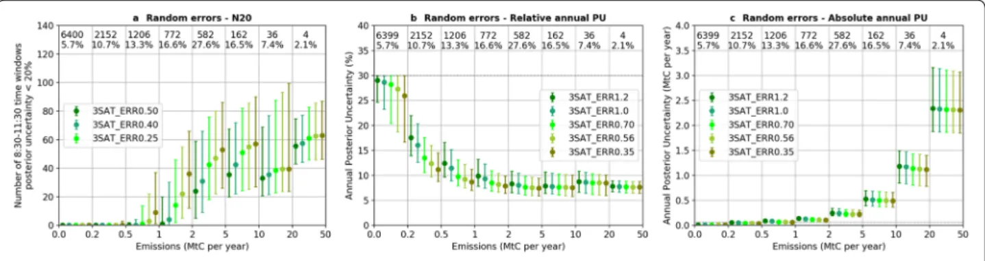
Figure 5 shows the median and interquartile range of

N20 (Fig. 5a) and annual posterior uncertainty (Fig. 5b and 5c) for the 300-km swath width 1-satellite constel-lation (1SAT_SWATH300) and for the 150-km swath width 2-satellite constellation (2SAT_SWATH150). The results show that multiplying the number of satel-lites while reducing the swath width by a factor of two has a negative impact on the performance of inversions for most bins of clumps. For example, the N20 median values are respectively 4/3, 13/10, 18/13, 14/9 for the 1–2, 2–5, 5–10 and 10–20 MtC per year emission bins

for 1SAT_SWATH300/2SAT_SWATH150 (Fig.  5a).

As a consequence, the annual posterior uncertainty

Fig. 4 Same as Fig. 2 but for relative (a) and absolute (b) posterior uncertainty in annual CO2 emissions for clumps in INV‑annual

Fig. 5 a Number of 8:30–11:30 time windows in a year for which the posterior uncertainty in the 3 h mean emissions are less than 20% (N20) in

INV‑3 h; b Relative posterior uncertainty in annual CO2 emissions in INV‑annual for 1 satellite with a swath width of 300 km (blue) and for 2 satellites

with a swath width of 150 km (purple); and c the same as b but for absolute values of posterior uncertainty. The results are binned according to the clump annual emission with bin limits given on the x‑axis of the figure. Numbers within the figure indicate the number of clumps in the bin and the fraction of total CO2 emissions generated by the clumps. Dots and error bars are the median and interquartile range of N20 (a) and posterior

are lower for 1SAT_SWATH300 than for 2SAT_ SWATH150. Having larger images with the 300  km swath allows to catch much larger portions of the plumes during the overpass which appears to be critical to pass the threshold of the 20% posterior uncertainties for most of the emission bins. The differences between the two constellation configurations are however less

than a few percent (Fig. 5b) within each emission bin.

There is an exception for the strongest emission bin (20–50 MtC per year) for which the N20 (annual pos-terior uncertainty) values are higher (lower) for 2SAT_ SWATH150 than for 1SAT_SWATH300, probably due to the statistical artefact of having only four clumps in this bin.

Figure 6 shows the median and interquartile range of

N20 (Fig. 6a) and annual posterior uncertainty (Fig. 6b and 6c) with different random measurement error for the three-satellite constellation. The results show that, as expected, increasing the precision of the instru-ments leads to an increase of the N20 values for most clumps. The increase is, however, more significant for the clumps whose annual emission budget is between 0.5 – 5 MtC per year than for those with larger annual emission budget. When the random measurement error is 1.2 ppm for vegetation albedo and SZA 50º, the N20 values for the sources within 0.5–1 MtC per year emis-sion bin decreases to zero. In addition, the annual poste-rior uncertainty decreases when random error is smaller, but the differences between the random error scenarios are of the order of a few tenths of a percent within each emission bin.

Discussion

PMIF was designed to permit a global evaluation of the impact of different configurations of satellite

constel-lations to constrain the CO2 emissions from localized

sources. Although some sources of uncertainties were not accounted for, such as diffuse emissions, the effect

of natural CO2 fluxes, systematic measurement error,

and error in using Gaussian plume model to represent atmospheric transport, PMIF can be used to investigate the first-order impacts of the configurations of satellite instruments and other key parameters in the inversion system, such as temporal error autocorrelation of the uncertainties in the emissions of clumps.

Our results confirm that the potential of a

constel-lation to monitor CO2 emissions is highly dependent

on the level of emissions of the clumps, as was shown by Wang et al. [35] with one satellite. It is found for all configurations with different numbers of satellites and instrument precision, a small city or thermal power plant with an annual budget lower than 0.5 MtC per year will not have any chance to have its emissions during 8:30– 11:30 time windows (in this study, e.g. 3 h before satellite overpasses) constrained to better than 20% by the satel-lite imagers like those planned for CO2M. Although the small clumps that will remain below the detection thresh-old are numerous (75.6% of all clumps), they only repre-sent 16.4% of the total clump CO2 emissions. Conversely,

clumps whose emissions are higher than 0.5 MtC per year have at least one 3 h (8:30–11:30) time window dur-ing which the emissions can be significantly constrained with a posterior uncertainty less than 20%. The N20 val-ues almost linearly increase with the number of satellites for all bins of clumps > 0.5 MtC per year. Improving ran-dom measurement error can also lead to an increase in the N20 values for clumps with emissions between 0.5–5 MtC per year, but its impact is relatively small compared to that of the number of satellites. Physically, the increase in the number of satellites increases the revisit frequency, and thus increase the N20 values, while an increase in the random measurement error will only improve the constraints on the same days as the reference inver-sion, resulting more precise posterior estimate (i.e. with smaller posterior uncertainty) of the 3 h emissions.

Because more satellites provide constraints on the 3 h emissions on more days, it is expected that the pos-terior uncertainty of the annual emission will improve

(i.e. decreases) as the number of satellites increases. At the same time, because more precise observations lead to more precise estimates of the 3 h emissions, it is also expected that these improved estimates of 3  h emis-sions could provide improved information about the clump emissions at longer period (e.g. annual emissions). Our results confirm this expected results, but both the increase in the number of satellites and the improvement in the precision of individual XCO2 retrievals only have

marginal benefit. This is due to the fact that the CO2M satellite observations only provide direct constraints on the emissions during 3  h before the overpasses for a limited number of days. The emissions is not directly constrained during the remaining 21  h and during the 8:30–11:30 on other days with no satellite observation sampling the plumes of clump emissions. In general, there are less than 70 occurrences when the emissions

during 8:30–11:30 are constrained (Fig. 6a, dark green

dots), the emissions in these time windows sum up to less than 10% of the annual emissions. The inversion system extrapolates the information on the emissions in 3 h time windows obtained from the observations, through the temporal auto-correlations between the prior uncertain-ties in emissions, to constrain the remaining 90% emis-sions. But the reliability of such extrapolation stays rather weak, leaving large residual error. This residual error, especially that in the emissions in the afternoon and night, will not reduce by simply adding more satellites sampling the plumes of emissions generated by emissions in the morning time (i.e. 8:30–11:30) or by improving the measurement precision. A combination of various LEO constellations with different crossing time could pro-vide more information on the emissions during different times of the day, and thus further improve the inversion performance. The geostationary-orbit (GEO) imagers,

such as GeoCARB [19, 23] or other GEO concepts [27,

28], can also offer frequent sampling of the plumes to

constrain the diurnal variations in the emissions. Satel-lites in a highly elliptical orbit (HEO) could provide con-tinuous or quasi-geostationary coverage of high latitudes

[21]. GEO and HEO satellites are thus also part of the

long-term vision of Europe [26] and of the Committee on

Earth Observation Satellites (CEOS) Constellation Archi-tecture [9] for CO2 monitoring from space. On the other

hand, Wang et al. [35] showed that the extrapolation from 3 h emissions to annual emissions is highly dependent on the assumption of temporal correlation between prior uncertainties. However, the temporal auto-correlations are poorly known in the emission inventories, and previ-ous studies selected the temporal auto-correlations in the prior uncertainty arbitrarily [16, 17]. Wang et al. [35] also showed that the exponential function commonly used by the inversion community might be a poor representation

of such temporal auto-correlations, highlighting the need of systematic assessments of the uncertainties in the emission products and its error structures.

Lastly, our study shows that having larger swath for individual satellites is advantageous to having more satel-lites for the monitoring of clump emissions at both 3 h

and annual scales (Fig. 5). Having larger swath and

hav-ing more satellites will both increase the samplhav-ing fre-quency, but the former option also allows for sampling a large portion of the plumes generated by clumps. Our study focuses on the use of data systematically taken on

nadir mode, which the most favorable over land [18]. The

monitoring of sources located near coasts could benefit from observations in glint mode. However, the width of the glint spot of CO2M should hardly exceed 30  km, which hampers the characterization of the plumes. Fur-thermore, this limitation of the effective images indicates that the benefit of having larger swath would be lost for the glint mode, for which having more satellites would be more critical. In addition, the observations in glint mode will also help in the global large-scale inversions of nat-ural fluxes, especially over the ocean, in which case it is more useful to have more satellites. It thus suggests that in the design of satellite missions, one should balance the costs among having more satellites, larger swath, and smaller measurement error, taking into account for the main target of the missions.

This study has investigated the capability of satellite

imagers to quantify the fossil fuel CO2 emissions from

large cities and point sources over one year. The capa-bility of these satellites to quantify long-term trends of emissions over several years has not been investigated.

Wang et  al. [33] showed that the uncertainties in the

trends of emissions are proportional to the uncertain-ties in the emissions of individual years. Qualitatively, the potential to estimate the emissions in the morning time increases proportionally increase with the number of satellites (Fig. 2), implying that the long-term trends in emissions in the morning time can be better estimated with more satellites. However, Fig. 4 showed that the pos-terior uncertainties in annual emissions are close to each other when having one to four satellites, indicating that the gain of having more satellites to estimate the trends in annual emissions are limited. This is related to the fact that there are large hour-to-hour, day-to-day, month-to-month and year-to-year variations in the emissions. The limited number of 3 h time windows for which the inversion yields small posterior uncertainties may hardly help distinguish these different sources of variations for the window 8:30–11:30, and even less for the emissions in the night and afternoon. To properly estimate the potential to estimate emission trends as a function of the

number of satellites, multi-year inversions accounting for these different sources of variations would be needed.

Conclusions

In this study, we use the PMIF global inversion system to assess the performance of a constellation of one to four

CO2M imagers to monitor anthropogenic CO2

emis-sions. Given the typical measurement precision of

indi-vidual retrievals of XCO2, the plumes from emission

sources with an annual emission smaller than 0.5 MtC can hardly be detected by satellite imagers. The number of time windows during which the emissions can be sig-nificantly constrained with a posterior uncertainty less than 20% is proportional to the number of satellites for clumps with an annual emission larger than 0.5 MtC.

The XCO2 observations from satellite imagers could

provide direct constraints on the estimate of emissions before the overpasses on clear-sky days, representing less than 10% of the annual emissions for a single clump. The emissions during other times are constrained through the temporal auto-correlations between the prior uncertain-ties. Improving the precision of individual retrievals will significantly improve the potential to constrain the emis-sions that are already well constrained in the reference simulation, whereas the improvement on the extrapola-tion of the constraints on the estimate of emissions in the afternoon and night is limited. As a result, the potential of the satellite imagers to monitor annual emissions is not proportional to the precision of individual retrievals. This study aslo shows that having larger swath for indi-vidual satellites is advantageous to having more satellites with narrower swaths.

Supplementary information

Supplementary information accompanies this paper at https ://doi. org/10.1186/s1302 1‑020‑00153 ‑4.

Additional file 1. Additional figures and tables. Abbreviations

LEO: Low‑Earth orbit; ESA: European Spatial Agency; CO2M: Carbon dioxide monitoring; XCO2: Vertically integrated columns of dry air mole fractions of

CO2; PMIF: Plume‑monitoring inversion framework; ODIAC: Open Source Data

Inventory of Anthropogenic CO2; CCMP: Cross‑calibrated multi‑platform; AMS:

Annual component and moderately correlated Sub‑annual component; SZA: Solar zenith angle; MODIS: Moderate Resolution Imaging Spectroradiometer; OSSE: Observing system simulation experiment.

Acknowledgements

We would like to thank Bernard Pinty for providing the vision of a CO2 Moni‑ toring and Verification Support (MVS) Capacity within the framework of the EU’s Copernicus Programme.

Authors’ contributions

PC, GB and FMB designed the research; YW and FL developed the PMIF code and made the analysis; MB and MR simulated the satellite sampling and random measurement noise for CarbonSat and the CO2M imagers; YW, GB,

FMB, FL, MB, MR, YM, AL, GJM, BZ and PC wrote the paper. All authors read and approved the final manuscript.

Funding

This work was mainly conducted and funded in the frame of the ESA project No.4000120184/17/NL/FF/mg. It also received support from the TRACE Indus‑ trial Chair (UVSQ / CEA / CNRS / Thales Alenia Space / TOTAL / SUEZ) ANR‑ 17‑CHIN‑0004 funded by the program « Chaires Industrielles 2017» of ANR. Y. W. also acknowledges support from Strategic Priority Research Program of Chinese Academy of Sciences “Science and Technology Project of Beautiful China Ecological Civilization Construction” (No. XDA23100400) and National Key Research and Development Program of China (2017YFA0605303).

Availability of data and materials

The source code for PMIFv1.0 for inversions with one satellite is published in Wang et al. [35]. The ODIAC inventory is available at https ://db.cger.nies.go.jp/ datas et/ODIAC /DL_odiac 2018.html. The clump dataset is available at https ://doi.org/10.6084/m9.figsh are.72177 26.v1. The wind fields from CCMP are available at https ://www.remss .com/measu remen ts/ccmp/. EDGAR v4.3.2 emission maps are needed to run the SectCS inversion, and are available at https ://edgar .jrc.ec.europ a.eu/overv iew.php?v=432_GHG.

Ethics approval and consent to participate

Not applicable.

Consent for publication

Not applicable.

Competing interests

The authors declare that they have no competing interests.

Author details

1 _{Laboratoire des Sciences du Climat et de L’Environnement, CEA‑CNRS, UVSQ‑}

Université Paris Saclay, Gif‑sur‑Yvette, France. 2 _{Canadian Centre for Meteoro‑}

logical and Environmental Prediction, 2121 Transcanada Highway, Dorval, QC H9P 1J3, Canada. 3 _{Key Laboratory of Land Surface Pattern and Simulation,}

Institute of Geographical Sciences and Natural Resources Research, Chinese Academy of Sciences, Beijing, China. 4 _{Institute of Environmental Physics}

(IUP), University of Bremen FB1, Otto Hahn Allee 1, 28334 Bremen, Germany.

5 _{European Space Agency (ESA), Noordwijk, Netherlands.} 6 _{Joint Research}

Centre, Directorate Sustainable Resources, European Commission, Transport & Climate, Via Fermi 2749, 21027 Ispra, Italy.

Received: 7 January 2020 Accepted: 26 August 2020

References

1. Andres RJ, Boden TA, Higdon DM. Gridded uncertainty in fossil fuel carbon dioxide emission maps, a CDIAC example. Atmos Chem Phys. 2016;16(23):14979–95.

2. Ars S, Broquet G, Yver Kwok C, Roustan Y, Wu L, Arzoumanian E, Bousquet P. Statistical atmospheric inversion of local gas emissions by coupling the tracer release technique and local‑scale transport modelling: a test case with controlled methane emissions. Atmosph Measur Techn. 2017;10(12):5017–37.

3. Atlas R, Hoffman RN, Ardizzone J, Leidner SM, Jusem JC, Smith DK, Gombos D. A cross‑calibrated, multiplatform ocean surface wind velocity product for meteorological and oceanographic applications. Bull Amer Meteor Soc. 2011;92(2):157–74.

4. Bovensmann H, Buchwitz M, Burrows JP, Reuter M, Krings T, Gerilowski K, et al. A remote sensing technique for global monitoring of power plant CO 2 emissions from space and related applications. Atmosph Measur Techniq. 2010;3(4):781–811.

5. Bréon FM, Broquet G, Puygrenier V, Chevallier F, Xueref‑Remy I, Ramonet M, et al. An attempt at estimating Paris area CO2 emissions from atmospheric concentration measurements. Atmos Chem Phys. 2015;15(4):1707–24.

6. Broquet G, Bréon F‑M, Renault E, Buchwitz M, Reuter M, Bovensmann H, et al. The potential of satellite spectro‑imagery for monitoring CO2 emissions from large cities. Atmos Meas Tech. 2018;11(2):681–708. 7. Buchwitz M, Reuter M, Bovensmann H, Pillai D, Heymann J, Schneising

O, et al. Carbon Monitoring Satellite (CarbonSat): assessment of atmos‑ pheric CO2 and CH4 retrieval errors by error parameterization. Atmos Meas Tech. 2013;6(12):3477–500.

8. Ciais P, Crisp D, Denier van der Gon HAC, Engelen R, Heimann M, Jans‑ sens‑Maenhout G, et al. Towards a European Operational Observing System to Monitor Fossil CO2 emissions. Brussels: European Commis‑ sion Directorate‑General for Internal Market, Industry, Entrepreneur‑ ship and SMEs Directorate I — Space Policy, Copernicus and Defence; 2015.

9. CEOS Atmospheric Composition Virtual Constellation Greenhouse Gas Team. A constellation architecture for monitoring carbon dioxide and methane from space. Report from the Committee on Earth Observa‑ tion Satellites (CEOS) Atmospheric Composition Virtual Constellation (AC‑VC). Available at https ://ceos.org/docum ent_manag ement /Virtu al_Const ellat ions/ACC/Docum ents/CEOS_AC‑VC_GHG_White _Paper _Versi on_1_20181 009.pdf. 2018.

10. Duren RM, Miller CE. Measuring the carbon emissions of megacities. Nat Clim Change. 2012;2:560–2.

11. Eldering A, Wennberg PO, Crisp D, Schimel DS, Gunson MR, Chatterjee A, Liu J, Schwandner FM, Sun Y, O’Dell CW, et al. The Orbiting Carbon Observatory‑2 early science investigations of regional carbon dioxide fluxes. Science. 2017;358(6360):5745.

12. ESA. Report for mission selection: CarbonSat‑An earth explorer to observe greenhouse gases. 2015. http://nora.nerc.ac.uk/id/eprin t/51401 2 Accessed 6 Oct 2016.

13. Gately CK, Hutyra LR. Large uncertainties in urban‑scale carbon emis‑ sions. J Geophys Res. 2017;122(20):11242–60.

14. Hedelius JK, Liu J, Oda T, Maksyutov S, Roehl CM, Iraci LT, Podolske JR, Hillyard PW, Liang J, Gurney KR, et al. Southern California meg‑ acity CO2, CH4, and CO flux estimates using ground‑ and space‑

based remote sensing and a Lagrangian model. Atmos Chem Phys. 2018;18:16271–91.

15. Hill T, Nassar R. Pixel size and revisit rate requirements for monitoring power plant CO2 emissions from space. Remote Sens. 2019;11(13):1608.

16. Kunik L, Mallia DV, Gurney KR, Mendoza DL, Oda T, Lin JC. Bayesian inverse estimation of urban CO2 emissions: Results from a synthetic data simulation over Salt Lake City, UT. Elem Sci Anth. 2019;7(1):36. 17. Lauvaux T, Miles NL, Deng A, Richardson SJ, Cambaliza MO, Davis KJ,

et al. High‑resolution atmospheric inversion of urban CO2 emissions during the dormant season of the Indianapolis Flux Experiment (INFLUX). J Geophys Res. 2015JD;121(10):2015JD024473. 18. Meijer Y. Copernicus CO2 Monitoring Mission Requirements Docu‑

ment. Report from Earth and Mission Science Division of European Space Agency. Available at https ://esamu ltime dia.esa.int/docs/Earth Obser vatio n/CO2M_MRD_v2.0_Issue d2019 0927.pdf. 2019. 19. Moore BI, Crowell SMR, Rayner PJ, Kumer J, O’Dell CW, O’Brien D,

Utembe S, Polonsky I, Schimel D, Lemen J. The Potential of the Geo‑ stationary Carbon Cycle Observatory (GeoCarb) to Provide Multi‑scale Constraints on the Carbon Cycle in the Americas. Front Environ Sci. 2018;6:109.

20. Nassar R, Napier‑Linton L, Gurney KR, Andres RJ, Oda T, Vogel FR, Deng F. Improving the temporal and spatial distribution of CO2 emissions from global fossil fuel emission data sets. J Geophys Res. 2013;118(2):917–33.

21. Nassar R, Sioris CE, Jones DBA, McConnell JC. Satellite observations of CO2 from a highly elliptical orbit for studies of the Arctic and boreal carbon cycle. J Geophys Res. 2014;119(5):2654–73.

22. Nassar R, Hill TG, McLinden CA, Wunch D, Jones DBA, Crisp D. Quantify‑ ing CO2 emissions from individual power plants from space. Geophys

Res Lett. 2017;44(10):10045–53.

23. O’Brien DM, Polonsky IN, Utembe SR, Rayner PJ. Potential of a geosta‑ tionary geoCARB mission to estimate surface emissions of CO2, CH4

and CO in a polluted urban environment: case study Shanghai. Atmos Meas Tech. 2016;9(9):4633–54.

24. Oda T, Maksyutov S, Andres RJ. The Open‑source Data Inventory for Anthropogenic CO2, version 2016 (ODIAC2016): a global monthly fossil fuel CO2 gridded emissions data product for tracer transport simula‑ tions and surface flux inversions. Earth Syst Sci Data. 2018;10(1):87–107. 25. Pillai D, Buchwitz M, Gerbig C, Koch T, Reuter M, Bovensmann H, et al.

Tracking city CO2 emissions from space using a high‑resolution inverse modelling approach: a case study for Berlin. Germany Atmos Chem Phys. 2016;16(15):9591–610.

26. Pinty B, Janssens‑Maenhout G, Dowell M, Zunker H, Brunhes T, Ciais P, Dee D, Denier van der Gon H, Dolman H, Drinkwater M, et al. An Opera‑ tional Anthropogenic CO2 Emissions Monitoring & Verification Support

capacity ‑ Baseline Requirements, Model Components and Functional Architecture (Brussels: European Commission Joint Research Centre). 2017.

27. Polonsky IN, Orien DM, Kumer JB, Oell CW. Performance of a geosta‑ tionary mission, geoCARB, to measure CO2, CH4 and CO column‑ averaged concentrations. Atmos Measure Technol. 2014;7(4):959–81. 28. Rayner PJ, Utembe SR, Crowell S. Constraining regional greenhouse

gas emissions using geostationary concentration measurements: a theoretical study. Atmosph Measure Techn. 2014;7(10):3285–93. 29. Reuter M, Buchwitz M, Schneising O, Krautwurst S, O’Dell CW, Richter

A, Bovensmann H, Burrows JP. Towards monitoring localized CO2 emissions from space: co‑located regional CO2 and NO2 enhance‑ ments observed by the OCO‑2 and S5P satellites. Atmos Chem Phys. 2019;19(14):9371–83.

30. Staufer J, Broquet G, Bréon F‑M, Puygrenier V, Chevallier F, Xueref‑Rémy I, Dieudonné E, Lopez M, Schmidt M, Ramonet M, et al. The first 1‑year‑ long estimate of the Paris region fossil fuel CO2 emissions based on atmospheric inversion. Atmos Chem Phys. 2016;16(22):14703–26. 31. Turnbull JC, Keller ED, Norris MW, Wiltshire RM. Independent evaluation

of point source fossil fuel CO2 emissions to better than 10%. Proc Natl Acad Sci U S A. 2016;113(37):10287–91.

32. Turnbull JC, Karion A, Davis KJ, Lauvaux T, Miles NL, Richardson SJ, Sweeney C, McKain K, Lehman SJ, Gurney KR, et al. Synthesis of Urban CO2 Emission Estimates from Multiple Methods from the Indianapolis Flux Project (INFLUX). Environ Sci Technol. 2019;53(1):287–95. 33. Wang Y, Broquet G, Ciais P, Chevallier F, Vogel F, Wu L, Yin Y, Wang R,

Tao S. Potential of European 14CO2 observation network to estimate the fossil fuel CO2 emissions via atmospheric inversions. Atmos Chem Phys. 2018;18(6):4229–500.

34. Velazco VA, Buchwitz M, Bovensmann H, Reuter M, Schneising O, Heymann JP, Krings T, Gerilowski K, Burrows JP. Towards space based verification of CO2 emissions from strong localized sources: fossil fuel power plant emissions as seen by a CarbonSat constellation. Atmosp Measur Techn. 2011;4(12):2809–22.

35. Wang Y, Broquet G, Bréon F‑M, Lespinas F, Buchwitz M, Reuter M, et al. PMIF v1.0: an inversion system to estimate the potential of satellite observations to monitor fossil fuel CO2 emissions over the globe. Geoscientific Model Development Discussions. 2020;1–27.

36. Wang Y, Ciais P, Broquet G, Bréon F‑M, Oda T, Lespinas F, et al. A global map of emission clumps for future monitoring of fossil fuel CO2 emis‑ sions from space. Earth Syst Sci Data. 2019;11(2):687–703.

37. Wu D, Lin JC, Oda T, Kort EA. Space‑based quantification of per capita CO2 emissions from cities. Environ Res Lett. 2020;15(3):035004. 38. Zheng B, Chevallier F, Ciais P, Broquet G, Wang Y, Lian J, Zhao Y.

Observing carbon dioxide emissions over China’s cities and industrial areas with the Orbiting Carbon Observatory‑2. Atmos Chem Phys. 2020;20(14):8501–10.

Publisher’s Note

Springer Nature remains neutral with regard to jurisdictional claims in pub‑ lished maps and institutional affiliations.