Physical characteristics and dynamics of the coastal Latex09 Eddy derived from in situ data and numerical modeling.

HAL Id: hal-00756955

https://hal.archives-ouvertes.fr/hal-00756955

Submitted on 24 Nov 2012

HAL is a multi-disciplinary open access

archive for the deposit and dissemination of

sci-L’archive ouverte pluridisciplinaire HAL, est destinée au dépôt et à la diffusion de documents

Latex09 Eddy derived from in situ data and numerical

modeling.

Marion Kersale, Anne Petrenko, Andrea Doglioli, I. Dekeyser, Francesco

Nencioli

To cite this version:

Marion Kersale, Anne Petrenko, Andrea Doglioli, I. Dekeyser, Francesco Nencioli. Physical char-acteristics and dynamics of the coastal Latex09 Eddy derived from in situ data and numerical modeling.. Journal of Geophysical Research. Oceans, Wiley-Blackwell, 2013, 118, pp.399-409. �10.1029/2012JC008229�. �hal-00756955�

Physical characteristics and dynamics of the coastal

1

Latex09 Eddy derived from in situ data and

2

numerical modeling.

3

M. Kersal´e,1 A. A. Petrenko,1 A. M. Doglioli,1 I. Dekeyser,1 F. Nencioli1

1_{Aix-Marseille Universit´e, Universit´e du}

Sud Toulon-Var, CNRS/INSU, IRD, MIO, UM 110, 13288, Marseille, Cedex 09, France.

Abstract.

4

We investigate the dynamics of a coastal anticyclonic eddy in the

west-5

ern part of the Gulf of Lion (GoL) in the northwestern Mediterranean Sea

6

during the Latex campaign in the summer 2009 (Latex09). The sampling

strat-7

egy combines SST satellite imagery, hull-mounted ADCP data, CTD casts

8

and drifter trajectories. Our measurements reveal an anticyclonic eddy

(La-9

tex09 eddy) with a diameter of ∼23 km and maximum depth of 31 m, cen-10

tered at 3◦_{34’E - 42}◦_{33’N. We use a high resolution, 3-dimensional,} primi-11

tive equation numerical model to investigate its generation process and

evo-12

lution. The model is able to reproduce the observed eddy, in particular its

13

size and position. The model results suggest that the Latex09 eddy is induced

14

by a large anticyclonic circulation in the northwestern part of the GoL, pushed

15

and squeezed toward the coast by a meander of the Northern Current. This

16

represents a new generation mechanism that has not been reported before.

17

The post generation dynamics of the eddy is also captured by the model. The

18

collision of the Latex09 eddy with Cape Creus results in a transient

struc-19

ture, which is depicted by the trajectories of two Lagrangian drifters

dur-20

ing Latex09. The transient structure and its advection lead to a transfer of

21

mass and vorticity from the GoL to the Catalan shelf, indicating the

impor-22

tance of mesoscale structures in modulating such exchanges in the region.

23

Keywords: Coastal eddies, in situ measurements, numerical modeling, mesoscale,

24

Gulf of Lion.

1. Introduction

Continental shelf processes are often affected by large eddies approaching the continental

26

slope from the deep ocean. In several open-ocean studies these energetic features of the

27

ocean circulation have been observed and described during their propagation onto the

28

continental shelf [Lewis and Kirwan Jr., 1985; Kirwan Jr. et al., 1988; Vukovich and

29

Waddel, 1991; Vidal et al., 1992; Richardson et al., 1994; Fratantoni et al., 1995; Hamilton

30

et al., 1999]. Studies that focus specifically on coastal eddies (the ones developed on the

31

continental shelf) are much scarcer.

32

Mitchelson-Jacob and Sundby [2001] have observed coastal eddies through the analysis

33

of satellite images on the continental shelf of Norway. They found that the size of these

34

eddies depends on the width of the fjord, with a diameter between 20 km to 60 km. An

35

anticyclonic eddy was sampled during a field campaign and followed by numerous drifters

36

[Mitchelson-Jacob and Sundby, 2001; Saetre, 1999]. This anticyclonic eddy appeared to

37

be a quasi-stationary feature [Eide, 1979], reaching 140 m depth. The wind direction, the

38

depth of the near-surface layer and the presence of stratification have been identified as

39

strong factors influencing the characteristics of these eddies. The strong currents in this

40

region have been linked directly to the formation of these eddies.

41

Mesoscale anticyclonic eddies have been also investigated inside the Gulf of Alaska.

42

These eddies are named according to the location of their generation: Sitka Eddies

43

[Tabata, 1982], Haida Eddies [Crawford and Whitney, 1999] and Yakutat Eddies [Ladd

44

et al., 2005]. They are baroclinic structures with a diameter of 150-300 km. These eddies

45

generally form in winter and detach from the continental margin in late winter and spring.

Haida Eddies usually form in the outflow of coastal waters [Crawford , 2002; Di Lorenzo

47

et al., 2005]. Sitka and Yakutat Eddies are believed to form in flow instabilities along the

48

continental slope [Melson et al., 1999].

49

Coastal cyclonic eddies have been also investigated further south along the British

50

Columbia shelf. The presence of a quasi-stationary eddy, the Juan de Fuca Eddy, on

51

the southern Vancouver Island shelf has been described in several studies [Tully, 1942;

52

Freeland and Denman, 1982; Denman and Freeland , 1985; Freeland and McIntosh, 1989;

53

MacFadyen et al., 2008]. This eddy is a topographically confined eddy which develops off

54

Cape Flattery in spring with a diameter of 80 km below 100 m depth.

55

Current separation from capes has been proposed as an explanation for eddy formation

56

in many coastal flows behind capes or headlands [Signell and Geyer , 1991; Doglioli et al.,

57

2004; Magaldi et al., 2010]. However, in the case of the buoyant flow around Cape Flattery,

58

the Coriolis force does not tend to maintain the current close to the coast [MacFadyen and

59

Hickey, 2010]. In fact, the eddy generation has been linked to two upwelling processes

60

occurring in the area with the important contribution of tidal forcing in the initial eddy

61

generation process [Foreman et al., 2008; MacFadyen and Hickey, 2010].

62

In general, the dynamics and the role of mesoscale coastal eddies are very complex

63

and different from one region to another. These eddies can translate away from their

64

generation region with the mean flow [Crawford et al., 2007; Mitchelson-Jacob and Sundby,

65

2001] or they can be quasi-stationary and linked to the topography [Eide, 1979; Freeland

66

and Denman, 1982]. Other studies highlight the role of mesoscale eddies on coastal

67

upwelling processes in idealized ecosystems [Lathuili`ere et al., 2010] or in the Ligurian Sea

68

[Casella et al., 2011]. In either case, they have profound impacts on local mechanisms

of water transport, vertical mixing and circulation processes. They are often biologically

70

rich regions because they can transport nutrient-rich coastal water off the coast to open

71

ocean.

72

The Gulf of Lion (GoL) is particularly relevant for the study of coastal mesoscale

struc-73

tures. The GoL is located in the northwestern Mediterranean Sea and is characterized by

74

a large continental margin (Figure 1). Its hydrodynamics is complex and highly variable

75

[Millot, 1990]. The circulation is strongly influenced by the Northern Current (NC), which

76

constitutes an effective dynamical barrier blocking coastal waters on the continental shelf

77

[Alb´erola et al., 1995; Sammari et al., 1995; Petrenko, 2003]. Exchanges between the GoL

78

and offshore waters are mainly induced by processes associated with the NC [Conan and

79

Millot, 1995; Flexas et al., 2002; Petrenko et al., 2005].

80

In the eastern part of the GoL, south of Marseilles, Allou et al. [2010] have observed the

81

presence of anticyclonic eddies between the NC and the coast using current meter data and

82

surface currents measured by High Frequency (HF) radars. The eddies are of diameters

83

12 to 28 km and they are coherent down to a depth of 140 m. Baroclinic instability of the

84

NC is a possible generation mechanism [Flexas et al., 2002]. Schaeffer et al. [2011] have

85

also observed anticyclonic eddies, with a diameter of 20-40 km, in the eastern part of the

86

GoL with HF radars and numerical simulations. They have shown that their generation

87

mechanism is related to the local wind conditions. After their generation, some of the

88

eddies are advected by the NC towards the western part of the shelf.

89

The instability of the NC and its role on the advection of eddies has been also proposed

90

to explain the presence of anticyclonic eddies on the Catalan continental shelf [Rubio et al.,

91

2005]. However Rubio et al. [2009a] rejected their previous hypothesis and suggested that

the process of flow separation due to a topographic barrier generates these eddies. A

93

possible mechanism for the generation of the Catalan eddies is described by Garreau

94

et al. [2011] in terms of release of potential energy from other eddies located in the GoL.

95

Through ADCP measurements and numerical simulations Estournel et al. [2003] showed

96

a large anticyclonic circulation located in the northwestern part of the GoL. In this part

97

of the GoL, a mesoscale anticyclonic circulation was first described by Millot [1979, 1982].

98

Hu et al. [2009, 2011a] showed the presence of a mesoscale eddy by a combined use of

99

data from satellite observations, in situ measurements and numerical modeling. The

100

eddies were baroclinic structures extending throughout the mixed layer (30 to 50 m),

101

often elliptical in shape and about 20-30 km in diameter (elliptical diameter is defined as

102

the mean of the minor and major axes). The generation process of the eddies mentioned

103

by Hu et al. [2009, 2011a] required two conditions: a persistent and strong northwest wind

104

and a strong stratification [Hu et al., 2011b].

105

The LAgrangian Transport EXperiment (LATEX) project (2008-2011) is designed to

106

study the mechanisms of formation of anticyclonic eddies and their influence on cross-shelf

107

exchanges in the western part of the GoL. The dynamics of mesoscale eddies is particularly

108

important in this part of the GoL since it represents a key region for regulating the outflow

109

from the continental shelf [Hu et al., 2011a; Nencioli et al., 2011].

110

The aim of the present study is to analyze the dynamical characteristics and generation

111

processes of such eddies during the summer of 2009. The methods used are described in

112

Section 2. Results based on a combination of satellite and in situ oceanographic data,

113

as well as numerical results are presented in Section 3. The general characteristics of the

observed eddies, their possible generation mechanisms and their behaviors are discussed

115

in Section 4.

116

2. Methods

The LATEX strategy was based on a combined use of Eulerian and Lagrangian in situ

117

measurements, satellite data and numerical modeling. The Latex09 campaign, conducted

118

from August 24 to 28, 2009 on board the R/V T´ethys II, was the second field experiment

119

of the LATEX project.

120

2.1. Data

Identifying the center of an eddy is one of the greatest challenges in the eddy

commu-121

nity. To characterize the observed eddy, this field campaign took advantage of various

122

observational data.

123

The data collected during Latex09 came from satellite, ship-based and drifter

obser-124

vations. Satellite data include SeaWiFs chlorophyll concentration [mg m−3_{] from the} 125

NASA’s Goddard Space Flight Center (GSFC) and Sea Surface brilliance Temperature

126

provided by M´et´eo-France (referred to as SSTb). During the campaign, the data were 127

sent to the R/V T´ethys II to help tracking the mesoscale features in near real-time.

128

A VMBB-150 kHz ship-based Acoustic Doppler Current Profiler (ADCP) was used to

129

measure current velocities (Figure 2). Following Petrenko et al. [2005], the instrument was

130

configured for recording 1 minute ensemble averages, providing horizontal currents with

131

a vertical resolution of 4 m from 11 to 247 m of depth. The software for ADCP raw data

132

treatment is provided by the French Institut National des Sciences de l’Univers (INSU

-133

CNRS) technical division. At each depth, the ADCP horizontal currents can be analyzed

in near real-time during the entire campaign using the method described by Nencioli

135

et al. _{[2008]. A searching grid of 30×30 points corresponding to a 30×30 km square area}

136

was imposed within each transect. Each grid point was tested as a possible location,

137

at that depth, for the center of the eddy. For each grid point, the components of the

138

ADCP velocities from a transect were decomposed into radial and tangential components

139

with respect to the reference frame centered at each point. The center, hereafter referred

140

to as single-depth transect center, was estimated as the grid point for which the mean

141

tangential velocity computed from the nearest ADCP records (black vectors - Figure 2)

142

was maximum.

143

In the present paper, the analysis focuses on Transect 1 and three other transects that

144

cross its center (Figure 2). Transect 2 is orthogonal to the coast (Figure 2b), Transect 3

145

is orthogonal to the continental slope (Figure 2c) and Transect 4 follows it (Figure 2d).

146

The start and end times for each transect are reported in Table 1.

147

During the transect mapping, we also collected a total of 25 profiles at specific locations

148

using a SeaBird SBE 19 CTD. We only show three of the CTD profiles, one inside the

149

eddy (CTD in, blue cross - Figure 5a), one at the edge (CTD edge, red cross) and one

150

outside the eddy (CTD out, black cross), representing eddy center, eddy edge and outside

151

conditions, respectively. Two satellite-tracked drifters, anchored at 15 m depth, were

152

deployed within the eddy to track the fluid motion. Drifter positions were provided by

153

the Argos system in quasi-real time. In addition, sea surface temperature, salinity and

154

fluorescence were measured continuously at the surface by the ship’s thermosalinometer

155

SBE 21.

2.2. Ocean model

In addition to the in situ measurements, the eddy dynamics have been investigated using

157

Symphonie, a 3-dimensional, primitive equation model, with a free sea surface, hybrid

158

sigma coordinates, based on Boussinesq and hydrostatic approximations [Marsaleix et al.,

159

2006, 2008]. We use the upwind-type advection-diffusion scheme adapted by Hu et al.

160

[2009] to improve the ability of the model to reproduce coastal mesoscale eddies in the

161

western part of the GoL. In the present study, the model is implemented over the whole

162

GoL with an horizontal resolution of 1 km × 1 km (Figure 1). The vertical discretization

163

consists of 40-hybrid vertical levels. The vertical resolution varies from 1 m in the upper

164

ocean to 40 m near the bottom.

165

This high resolution model is one-way nested to a coarse grid model (3 km × 3 km)

166

covering a larger domain. The initial and open boundary conditions for the larger domain

167

are provided by the Mediterranean Forecasting System (MFS) general circulation model

168

[Pinardi , 2003] with a resolution of 1/8◦_{. The atmospheric forcing is obtained from the} 169

3-hr outputs of the meteorological model Aladin of M´et´eo-France with a spatial resolution

170

of 0.1◦_×0.1◦_{. The daily fresh water fluxes from the major rivers are taken into account.} 171

The readers are referred to Hu et al. [2011b] for more details about the model settings.

172

This model was run from 2001 to 2008 and the results were analyzed by Hu et al.

173

[2011b]. In the present study it is run for 2009, with a restart from the previous simulation.

174

The daily outputs of current velocity components, salinity, temperature and density are

175

averaged over 24 hours of simulation, to filter out the diurnal cycle. We have verified that

176

the 24-hours average is also effective in filtering out the inertial oscillations, that is of

∼17.5 hours in the GoL. The remaining unfiltered inertial kinetic energy represents 1-5% 178

of the total average kinetic energy.

179

In order to study the generation process with the same criteria used in the study of Hu

180

et al. [2011a], we consider the wind as a strong and persistent northwesterly wind event

181

when its amplitude is larger than, or equal to, 8 m s−1_{, and its direction is between 270}◦ 182

and 360◦ _{for at least 75% of the time during the last three days. In order to investigate} 183

the variation of stratification, the potential energy anomaly φ is chosen as the indicator of

184

the stability of the water column [Hu et al., 2011a; Burchard and Burchard , 2008; De Boer

185

et al., 2008]. The value of φ decreases with the level of homogeneity through the water

186

column. Values of φ reaching 20 J m−3 _{(100 J m}−3_{) indicate a weak (strong) stratification.} 187

An intermediate stratification is defined with a value φ around 60 J m−3_. 188

The utility program WATERS [Doglioli et al., 2007] is used to objectively identify and

189

follow the coherent eddy structures in our numerical simulations. This automatic

detec-190

tion of 3-dimensional eddy structures was first conducted with a high-resolution numerical

191

model of the oceanic region around South Africa [Doglioli et al., 2007]. More recently,

192

WATERS has been used by Rubio et al. [2009b] to investigate mesoscale activity in the

193

Benguela upwelling system and by Dencausse et al. [2010] to study the routes of Agulhas

194

rings. In the South Atlantic Ocean, Souza et al. [2011] also tested the performances of

195

WATERS in comparison with other automatic identification algorithms for the

quantifi-196

cation and characterization of mesoscale eddies. In coastal waters, Hu et al. [2009, 2011b]

197

successfully used WATERS to identify anticyclonic eddies in the GoL. The method is

198

based on wavelet analysis of horizontal slices of modeled relative vorticity to extract

co-199

herent structures, providing a set of grid points and a center associated to each eddy. The

center of the modeled eddy is defined as the maximum in magnitude of relative vorticity.

201

For each eddy, tracking can be performed both backward and forward in time to find the

202

“birth” and the “death” of the eddy. At each time step, the eddy’s diameter, D, is defined

203

as the average between the zonal (DEW_{) and the meridional (D}N S_{) cords that intercept} 204

each eddy center with both endpoints on the edge of the structure. This definition

ac-205

counts for stretched shapes. The analysis is repeated at each depth level (k) to diagnose

206

the vertical extent of the identified eddy. The vertical tracking ends at the level number

207

(iz) before the eddy signal in relative vorticity becomes too weak to be detected. With 208

this method the reference diameter can be calculated as :

209 D= 1 iz iz X k=1 DEW k + DkN S 2 (1) 210

For stretched eddies, the variance made on the calculation of D with eq(1) is estimated

211 as: 212 Dvar = 1 iz iz X k=1 DEW k + DkN S 2 − D !2 (2) 213

In the following, our results are written as D ±√Dvar. 214

3. Results

3.1. In situ experiment

An eddy was detected before the campaign from the analysis of the SSTb and SeaWiFs 215

chlorophyll-a surface concentration. On August 20, lower SSTb (∆ SSTb = 1.5◦C) and 216

lower chlorophyll-a concentration (∆ Chla = 0.4 mg m−3) within the eddy relative to the 217

surroundings, allowed for its identification. The eddy’s center position was estimated to

218

be 3◦_30’E-42◦_{36’N. At the beginning of the campaign, during Transect 1, we crossed the} 219

whole eddy, passing through its satellite eddy center.

On the basis of ADCP velocities, the single-depth transect center for Transect 1 at 15 m

221

depth C1 15 was estimated to be at 3◦_{33’E - 42}◦_{33’N (black cross - Figure 2a).} Succes-222

sively, we conducted a systematic mapping of the eddy by performing several transects

223

passing through that position.

224

ADCP horizontal current velocity vectors at 15 m depth reveal a clockwise circulation

225

associated with an anticyclonic eddy (Figure 2). We also detect a strong current with

226

a southwestward direction at the southeastern part of the eddy, corresponding to the

227

presence of the NC (Figures 2b,c).

228

Tangential velocity at 15 m depth and surface temperature measured during Transect

229

3 are shown in Figure 3 with respect to the distance from the single-depth transect center

230

for Transect 3 at 15 m depth (C3 15 - black cross - Figure 2c). Since Transect 3 did not

231

pass directly through C3 15, the data are measured only up to a distance of 1.4 km from

232

it. At this distance, the values of tangential velocities are not zero but close to zero. Then

233

they increase linearly with radial distance to reach maximum values of about 0.4 m s−1 234

at roughly 9 km (15 km) for the northwestern (southeastern) part of the transect. These

235

values show that the eddy is not symmetric. After reaching the maximum values, the

236

tangential velocities slowly decrease as the radial distance further increases. The portion

237

of the eddy characterized by a constant angular velocity corresponds to the portion of the

238

eddy that rotates as a solid body (dashed line - Figure 3a). Thus the distance between

239

the two maximum values of tangential velocities at the edges of the eddy, evaluated to be

240

∼24 km (9 km +15 km), represents the diameter of the solid body rotation of the eddy. 241

The distribution of surface temperature from the thermosalinometer, with respect to

242

radial distance from C3 15, shows warmer waters at the southeastern border of the eddy

(Figure 3b). The plot shows the presence of a strong temperature gradient (more than

244

1◦_{C over a distance of ∼3 km). This sudden temperature increase is located at 15 km} 245

from C3 15, and coincides with the maximum value of tangential velocity component, and

246

hence the edge of the solid-body part of the eddy.

247

The vertical section of tangential velocity in Figure 4a, between 11 and 19 m depth,

248

shows a typical eddy structure with two lobes of relatively high positive tangential

ve-249

locities that extend on the two sides of the axis. A common feature for the tangential

250

velocities at these depths is a quite rapid increase from the single-depth transect center

251

for Transect 3 up to a distance of 10-15 km where they reach their maximum values.

252

Between 19 and 31 m depth, tangential velocities never reach near zero values close to the

253

single-depth transect center for Transect 3, as those at shallower depths do. This occurs

254

because the deeper positions of the single-depth transect centers for Transect 3 tend to be

255

further away from the transect (Figure 4b), indicating that the axis of the eddy is tilted.

256

Below 31 m depth, velocities decay relatively rapidly with depth, so that the anticyclonic

257

circulation associated with the eddy is limited to the upper 31 m. At deeper depths,

258

the presence of the NC is most distinguishable between 3◦_{42’E and 3}◦_{46’E with velocities} 259

around 0.2 m s−1_{. The impact of the NC on the anticyclonic eddy is also obvious from} 260

the higher tangential velocities on its southeastern part at the surface.

261

In the preceding section we have only presented the analysis of Transect 3 at 15 m

262

depth, since similar evaluations made for all the other transects gave similar results.

263

Tangential velocities with respect to radial distance from the single-depth transect center

264

have been analyzed for all the transects at three depths (11 m, 15 m, 19 m). These

265

depths have been chosen because they are the shallowest bins available from the ADCP

and are within the studied eddy. The resulting estimations of the diameter and the

267

position of the single-depth transect centers are summarized in Table 2. In the table we

268

introduce two other center estimates. The depth-averaged transect centers are defined

269

as the mean of the positions of the single-depth transect centers. The transect-averaged

270

eddy center, hereafter named for simplification eddy center C, is defined as the mean of

271

the positions of the depth-averaged transect centers. The estimated position of the eddy

272

center corresponds to the depth-averaged transect center for Transect 1 (C1-Table 2).

273

Transects 3 and 4 are approximately meridional and zonal, respectively, and thus they

274

are also roughly perpendicular (Figure 2). Therefore, in order to estimate the diameter

275

from in situ data, we apply eq(1) where DEW (DN S) is the distance between the two 276

maximum values of tangential velocities on Transect 3 (4) at the three reference depths

277

(11 m, 15 m, 19 m). The diameter of the eddy is thereby estimated to be 22.7±1.2 km.

278

Another way to evaluate the vertical extension of the eddy comes from the analysis of the

279

vertical profiles of temperature and fluorescence (Figure 5). The temperature profiles show

280

values between 23.0◦_{C and 23.6}◦_{C at the surface and a progressive decrease with depth} 281

to a value of 13.4◦_{C at about 150 m depth (Figure 5b). A strong thermocline is observed} 282

between 8 and 18 m (20 and 35 m), at station CTD out (CTD in), outside (inside) the

283

eddy. Indeed the anticyclonic eddy corresponds to a deepening of the thermocline. We

284

also notice a weak value of fluorescence at the surface for all three profiles (Figure 5c). A

285

fluorescence peak reaching 2.5 µg l−1 _{is visible at 50 m depth outside the eddy (station} 286

CTD out); it decreases to less than 2 µg l−1 _{at the edge of the eddy (station CTD edge).} 287

Only a faint maximum of 0.6 µg l−1 _{can be found at 70 m depth inside the eddy (station} 288

CTD in), deeper than the thermocline. This agrees with a reduced phytoplankton biomass

289

induced by the downwelling associated with anticyclonic eddies [Siegel et al., 2011].

290

3.2. Modeling results

The study of the numerical model outputs with the wavelet analysis allows us to retrieve

291

information about the various mesoscale structures in the study area in 2009. Hereafter,

292

we adopt the terminology introduced by Hu et al. [2011b] who defined “long-life” eddies

293

as the ones which last for at least 15 days. We have thoroughly studied year 2009 and two

294

modeled “long-life” anticyclonic eddies are identified. The wavelet analysis shows that

295

the first “long-life” eddy (hereafter A1 ) is generated on June 28 and lasts until July 20,

296

while the second eddy is generated on August 16 and lasts until October 12. The latter is

297

considered to be analogous to the eddy sampled during Latex09 and described in Section

298

3.1, and hence is hereafter referred to as A2-Latex09.

299

First, we want to understand the generation mechanism of these two eddies. The

300

generation process of eddy A1 starts with a strong northwesterly wind observed from

301

June 19 to 21. This strong wind, with an amplitude equal to 18 m s−1_{, induces an Ekman} 302

transport piling the water close to Cape Creus. Then a northward current along the

303

Roussillon coast starts on June 26. The closing of this Ekman southwestward drift and

304

coastal current jet generates the anticyclonic eddy. An intermediate stratification has also

305

been identified with an absolute value of potential energy anomaly more than 60 J m−3_. 306

These facts indicate that the generation process of the eddy A1 corresponds to the one

307

described by Hu et al. [2011b] for all “long-life” eddies between 2001 and 2008.

308

On the other hand, the generation process of the second eddy, A2-Latex09, is different.

309

During a weak wind event (Figure 6a), we first observe the generation of a large-scale

anticyclonic circulation extending to all the western GoL on July 20 (Figure 6e). In

311

the western part of the GoL, the positive sea surface height (Figure 6f) corresponds

312

to an anticyclonic circulation extending south of Cape Creus. A meander of the NC

313

approaches this large anticyclonic circulation, squeezing it and reinforcing the current at

314

its southeastern edge. This occurs during a northwesterly wind event (Figure 6b) that

315

started on August 6. It produces a localized upwelling south of Cape d’Agde but smaller

316

than the one observed in the generation process proposed by Hu et al. [2011b]. During

317

this generation process, the wind can be classified on August 27 as a strong northwesterly

318

wind event (16 m s−1_{) but not persistent since its occurrence during the last three days} 319

is less than 75%. A strong stratification has also been identified with an absolute value

320

of potential energy anomaly more than 100 J m−3_{. On August 16 the wavelet analysis} 321

identifies two anticyclonic eddies corresponding to the zonal separation of the anticyclonic

322

area in two smaller areas (Figure 6g). Indeed the NC meander seems to push and squeeze

323

the structure to the west. Then, as the presence of the coast blocks its progression, the

324

structure becomes separated in two structures: one eddy on the shelf of the GoL

(A2-325

Latex09) and one moving inside the Catalan Basin. On August 27, these structures are

326

clearly distinct (Figure 6h). In the following, the eddy in the Catalan shelf is referred to

327

as the Catalan Eddy.

328

In the next paragraphs, the characteristics of A2-Latex09 on August 27 are presented

329

for comparison with the in-situ data sampled at the same time (Table 1). The modeled

330

A2-Latex09 extends throughout the mixed layer until 37 m depth. The wavelet analysis

331

identifies an eddy centered at 3◦_26’E-42◦_{36’N with a diameter of 28.6±1.4 km. The} 332

position of the eddy’s center is calculated as the mean of its positions between 1 and 37 m

depth with a vertical step of 4 m. This vertical step is chosen to be equal to the vertical

334

resolution of the ADCP for a better comparison. The diameter of the eddy is obtained

335

applying eq(1) and (2) to North/South and East/West transects across the modeled eddy

336

with the same vertical resolution between the same depth interval.

337

Moreover the model has been also useful to examine the post generation mechanism of

338

A2-Latex09. Indeed on August 31, A2-Latex09 encounters Cape Creus. Following this

339

event, a transient anticyclonic structure is generated downstream the cape on September

340

3, detaching from A2-Latex09. A 3D view of potential vorticity (Figure 7) in the domain

341

gives a good visualization of the phenomenon. In order to quantify the transfer, a balance

342

of mass has been computed from the model results between August 30 and September 3.

343

The transient structure represents ∼33% of the A2-Latex09 ’s mass. The loss of mass of 344

the eddy A2-Latex09 is estimated to be ∼41%. As a result, 8% of the mass is dispersed 345

during this separation. The gain expected on the mass of the Catalan Eddy can not be

346

estimated properly since the latter is too close to the model domain boundary.

347

A 2D view of the relative vorticity (Figure 8a) shows the presence of the transient

an-348

ticyclonic structure between A2-Latex09 and the Catalan Eddy. The dynamics simulated

349

by the model is supported by the trajectories of two Lagrangian drifters, released during

350

the Latex09 campaign, from August 26 to September 12 (Figure 8b). On August 26,

351

drifter No. 83631 (blue line) was deployed near the eddy center C and drifter No. 83632

352

(purple line) near the western outer edge of the eddy. Drifter No. 83631 made one full

353

loop around the eddy in 81 hours. Its trajectory stopped looping around the eddy on

354

September 2 and then drifted northward. Drifter No. 83632 started to loop around the

355

eddy but, on August 30, it began to drift southward moving away from it. Checking the

rotation period of this buoy to ascertain the nature of this feature, we found a rotation

pe-357

riod of 39 hours, corresponding approximately to half the rotation period of A2-Latex09.

358

This rotation does not correspond to an inertial oscillation, which has a typical period of

359

∼17.5 hours in the GoL. This fact confirms the hypothesis that the drifter is trapped in 360

the transient structure. On September 6, Drifter No. 83632 got trapped in the Catalan

361

Eddy located at 3◦_11’E-41◦_35’N. 362

4. Discussion and Concluding remarks

The generation and characteristics of a coastal anticyclonic eddy detected in the western

363

part of the GoL have been studied from a combination of in situ measurements and

364

numerical modeling from the end of August 2009 to the middle of October 2009.

365

On the basis of in situ measurements, the anticyclonic eddy is centered at 3◦ 34’E-366

42◦_{33’N and is characterized by a diameter of 22.7±1.2 km, reaching a maximal depth of} 367

31 m. The observed anticyclonic eddy is well reproduced by the model as shown by the

368

numerical relative vorticity field on September 3 (Figure 8a). The major characteristics

369

of this modeled eddy agree with the observations, although its horizontal dimensions are

370

slightly larger than the observed ones. The diameter of the simulated eddy is 28.6±1.4 km.

371

This eddy is approximately situated at the same location as the measured one, slightly

372

more northwestward (3◦_26’E-42◦_36’N). 373

To characterize the dynamics of the eddy, we computed the local Rossby number (Ro = 374

Vmax

Rmaxf) and the the Rossby radius of deformation (Rd=

√

g′_H′

f ). Vmax is calculated as the 375

mean of the maximum tangential velocities on Transects 3 and 4 at the three reference

376

depths. Rmax is calculated as half of the reference diameter D, defined in eq(1). With 377

the eddy is 0.26. To compute Rd, the reduced gravity was calculated as g′ = ρ2_ρ−ρ1

2 g, with

379

ρ₂ = 1029.04 kg m−3_{, the mean density below the mixed layer, and ρ}

1 = 1025.75 kg m−3, 380

the mean density within the mixed layer. The mixed layer depth was 10.9 m. The resulting

381

Rd is 5.9 km, which is smaller than the eddy reference radius Rmax. Since Rmax >Rd, we 382

can objectively classify the eddy as a mesoscale structure. Since the local Rossby number

383

is not small, its dynamics can not be approximated by quasi-geostrophic theory.

384

We can compare our results with the data gathered during the experiment Latex08 in

385

the same area [Hu et al., 2011a] conducted from September 1 to 5, 2008. Although the

386

generation process is different, these two coastal anticyclonic eddies have similar

charac-387

teristics in terms of position, extension and dynamical characteristics. This fact shows

388

the important influence of coast and bathymetry on the physical characteristics of these

389

mesoscale eddies.

390

Hu et al. [2011a] emphasized that the 2008 eddy interacts with the Northern Current

391

at the end of the Latex08 campaign, leading to its deformation and maybe to its death.

392

In our case, the presence and role of the Northern Current is much clearer (Figures 2b,c).

393

The NC has first created the eddy and then it affected it, reinforcing the current at its

394

southeastern part. This intensification could explain the asymmetric shape of the eddy.

395

Regarding the possible mechanisms for the formation of these anticyclonic eddies in the

396

literature, a few processes of generation have been listed in the introduction. The

numer-397

ical study of eddy generation in the western part of the GoL by Hu et al. [2011b] shows

398

that these eddies need two conditions to be generated: a persistent and strong northwest

399

wind and a strong stratification. This mechanism of generation has been identified in our

400

analysis. Indeed, the process of generation of the first modeled anticyclonic eddy A1

responds to Hu et al. [2011b]’s process with the two conditions described above. A strong

402

northwesterly wind is observed from June 19 to 21 and an intermediate stratification is

403

noted at the end of June with an absolute value of potential energy anomaly greater than

404

60 J m−3_. 405

Instead, for anticyclonic eddy A2-Latex09, we propose a new process of generation,

as-406

sociated with the NC. This new mechanism starts with the generation of an anticyclonic

407

circulation extending over a large part of the coastal area (Figure 6e). The generation of

408

this anticyclonic circulation, precursor to the eddy, is not analyzed in this study but it

409

could have been generated by the mechanism proposed by Hu et al. [2011b]. Interaction

410

with a meander of the Northern Current and the presence of the coast induces the

latitu-411

dinal separation of this anticyclonic circulation into two eddies, the northern one in the

412

GoL and the southern one on the Catalan shelf. To our knowledge, this generation process

413

has not been proposed before. Indeed the combined analysis of Rubio et al. [2005, 2009a]

414

suggests that Catalan eddies are generated downstream of Cape Creus as a result of a

415

flow separation triggered by an intense northwest wind event in the GoL. While Garreau

416

et al.[2011] indicate that GoL eddies flow southward creating Catalan eddies after a burst

417

of southeasterlies and northerlies. The authors conclude that the death of GoL eddies is

418

clearly linked to the birth of strong Catalan eddies. In our case, the detachment of a part

419

of the eddy does not lead to the death of A2-Latex09. The formation of this transient

420

structure comes from the encounter of the A2-Latex09 with Cape Creus. The generation

421

of this transient structure causes a loss of mass and vorticity for A2-Latex09. In the in-situ

422

measurements, a small structure is detected in the same spatial area and at the same time

423

(Figure 8b) as the one given by the model (Figure 8a). When drifter No. 83632 starts

to loop outside the eddy (Figure 8b), drifting toward the south, its rotation period (39

425

hours) eliminates the occurrence of an inertial oscillation. After ∼6 days this drifter is 426

caught by the Catalan Eddy located at 3◦_11’E-41◦_{35’N. The generation of the transient} 427

structure moving from A2-Latex09 toward the Catalan Eddy in the model results can

428

explain the trajectories of these drifters. From the in-situ experiment it is clear that the

429

generation of this structure leads directly to a transfer of mass from the eddy of the GoL

430

to the eddy of the Catalan shelf.

431

This study gives a more complete and consistent picture of the GoL coastal eddy

dy-432

namics. A full 3D analysis from numerical simulation will be made with the objective

433

of better understanding the remaining open questions about the generation of the

an-434

ticyclonic circulation, first step of the proposed new generation process. Besides, this

435

numerical modeling work would be useful to explore the coupled physical and

biogeo-436

chemical dynamics at mesoscale and the role of mesoscale eddies in the transfers between

437

the GoL coastal zone and the neighboring coastal regions.

438

Acknowledgments. The LATEX project is supported by the programs LEFE/IDAO

439

and LEFE/CYBER of the INSU-Institut National des Sciences de l’Univers and by the

440

Region PACA-Provence Alpes Cˆote d’Azur. The meteorological data were kindly supplied

441

by M´et´eo-France. We acknowledge the MFS program for OGCM outputs. We are warmly

442

grateful to the crews of the R/V T´ethys II for their assistance. We thank Z. Y. Hu for

443

providing the last configuration of the model. The authors want to thank J. Bouffard and

444

C. Yohia for precious comments and useful discussions. Marion Kersal´e is financed by a

445

MENRT Ph.D. grant.

References

Alb´erola, C., C. Millot, and J. Font (1995), On the seasonal and mesoscale variabilities of

447

the Northern Current during the PRIMO-0 experiment in the western Mediterranean

448

Sea, Oceanol. Acta, 18 (2), 163–192.

449

Allou, A., P. Forget, and J. L. Devenon (2010), Submesoscale vortex strucures at the

450

entrance of the Gulf of Lions in the Northwestern Mediterranean Sea, Cont. Shelf Res.,

451

30, 724–732, doi:10.1016/j.csr.2010.01.006.

452

Burchard, H., and R. Burchard (2008), A dynamic equation for the potential energy

453

anomaly for analysing mixing and stratification in estuaries and coastal seas, Estuarine,

454

Coastal Shelf Science, 77 (4), 679–687, doi:10.1016/j.ecss.2007.10.025.

455

Casella, E., A. Molcard, and A. Provenzale (2011), Mesoscale vortices in the Ligurian

456

Sea and their effect on coastal upwelling processes, J. Mar. Sys., 88 (1), 12–19, doi:

457

10.1016/j.jmarsys.2011.02.019.

458

Conan, P., and C. Millot (1995), Variability of the Northern Current off Marseilles, western

459

Mediterranean Sea, from February to June 1992, Oceanol. Acta, 18 (2), 193–205.

460

Crawford, W. R. (2002), Physical characteristics of Haida Eddies, Journal of

Oceanogra-461

phy, 58 (5), 703–713, doi:10.1023/A:1022898424333.

462

Crawford, W. R., and F. A. Whitney (1999), Mesoscale eddy aswirl with data in Gulf of

463

Alaska Ocean, Eos, Trans. AGU, 80 (33), 365–670.

464

Crawford, W. R., P. J. Brickley, and A. C. Thomas (2007), Mesoscale eddies dominate

465

surface phytoplankton in northern Gulf of Alaska, Prog. Oceanogr., 75, 287–303, doi:

466

10.1016/j.pocean.2007.08.016.

De Boer, G. J., J. D. Pietrzak, and J. C. Winterwerp (2008), Using the potential energy

468

anomaly equation to investigate tidal straining and advection of stratification in a region

469

of freshwater influence, Ocean Model., 22, 1–11.

470

Dencausse, G. J., M. Arhan, and S. Speich (2010), Routes of agulhas rings in the south

471

eastern cape basin, Deep-Sea Res. I, 57, 1406–1421, doi:10.1016/j.dsr.2010.07.008.

472

Denman, K. L., and H. J. Freeland (1985), Correlation scales, objective mapping and a

473

statistical test of geostrophy over the continental shelf, J. Mar. Res., 43 (3), 517–539,

474

doi:10.1357/002224085788440402.

475

Di Lorenzo, E., M. G. G. Foreman, and W. R. Crawford (2005), Modelling the generation

476

of Haida Eddies, Deep-Sea Res. II, 52, 853–873, doi:10.1016/j.dsr2.2005.02.007.

477

Doglioli, A. M., A. Griffa, and M. G. Magaldi (2004), Numerical study of a coastal current

478

on a steep slope in presence of a cape: The case of the Promontorio di Portofino,

479

J. Geophys. Res., 109, C12033, doi:10.1029/2004JC002422.

480

Doglioli, A. M., B. Blanke, S. Speich, and G. Lapeyre (2007), Tracking coherent structures

481

in a regional ocean model with wavelet analysis: application to Cape Basin Eddies,

482

J. Geophys. Res., 112, C05043, doi:10.1029/2006JC003952.

483

Eide, L. I. (1979), Evidence of a topographically trapped vortex on the Norwegian

conti-484

nental shelf, Deep-Sea Res. I, 26 (6), 601–621, doi:10.1016/0198-0149(79)90036-0.

485

Estournel, C., X. Durrieu de Madron, P. Marsaleix, F. Auclair, C. Julliand, and R.

Ve-486

hil (2003), Observation and modeling of the winter coastal oceanic circulation in the

487

Gulf of Lion under wind conditions influenced by the continental orography (FETCH

488

experiment), J. Geophys. Res., 108 (C3), 8059, doi:10.1029/2001JC000825.

Flexas, M. M., X. Durrieu de Madron, M. A. Garcia, M. Canals, and P. Arnau (2002),

490

Flow variability in the Gulf of Lions during the MATER HFF experiment (March-May

491

1997), J. Mar. Sys., 33-34, 197–214, doi:DOI: 10.1016/S0924-7963(02)00059-3.

492

Foreman, M. G. G., W. Callendar, A. MacFadyen, B. M. Hickey, R. E. Thomson, and

493

E. Di Lorenzo (2008), Modeling the generation of the juan de fuca eddy, J.

Geo-494

phys. Res., 113 (C03006), doi:10.1029/2006JC004082.

495

Fratantoni, D. M., W. E. Johns, and T. L. Townsend (1995), Rings of the North Brazil

496

Currents: their structure and behavior inferred from observations and a numerical

sim-497

ulation, J. Geophys. Res., 100 (C6), 10.633–10.654, doi:10.1029/95JC00925.

498

Freeland, H. J., and K. L. Denman (1982), A topographically controlled upwelling center

499

off southern Vancouver Island, J. Mar. Sys., 40 (4), 1069–1093.

500

Freeland, H. J., and P. McIntosh (1989), The vorticity balance on the southern British

501

Columbia continental shelf, Atmos.-Ocean, 27 (4), 643–657.

502

Garreau, P., V. Garnier, and A. Schaeffer (2011), Eddy resolving modelling of the Gulf of

503

Lions ans Catalan Sea, Ocean Dynam., 61, 991–1003, doi:10.007/s10236-011-0399-2.

504

Hamilton, P., G. S. Fargion, and D. C. Biggs (1999), Loop Current eddy paths in

505

the western Gulf of Mexico, J. Phys. Oceanogr., 29 (6), 1180–1207,

doi:10.1175/1520-506

0485(1999)029¡1180:LCEPIT¿2.0.CO;2.

507

Hu, Z. Y., A. A. Doglioli, A. M. Petrenko, P. Marsaleix, and I. Dekeyser (2009),

Nu-508

merical simulations of eddies in the Gulf of Lion, Ocean Model., 28 (4), 203 – 208,

509

doi:10.1016/j.ocemod.2009.02.004.

510

Hu, Z. Y., A. A. Petrenko, A. M. Doglioli, and I. Dekeyser (2011a), Study of mesoscale

511

anticyclonic eddy in the western part of the Gulf of Lion, J. Mar. Sys., 88, 3–11, doi:

10.1016/j.jmarsys.2011.02.008.

513

Hu, Z. Y., A. A. Petrenko, A. M. Doglioli, and I. Dekeyser (2011b), Numerical study of

514

eddy generation in the western part of the Gulf of Lion, J. Geophys. Res., 116, C12030,

515

doi:10.1029/2011JC007074.

516

Kirwan Jr., A. D., J. K. Lewis, A. W. Indest, P. Reinersman, and I. Quintero (1988),

517

Observed and Simulated Kinematic Properties of Loop Current Rings, J. Geophys. Res.,

518

93(C2), 1189–1198, doi:10.1029/JC093iC02p01189.

519

Ladd, C. M., N. B. Kachel, C. W. Mordy, and P. J. Stabeno (2005), Observations from

520

a Yakutat eddy in the northern Gulf of Alaska, J. Geophys. Res., 110 (C03003), doi:

521

10.1029/2004JC002710.

522

Lathuili`ere, C., V. Echevin, M. L´evy, and G. Madec (2010), On the role of the mesoscale

523

circulation on an idealized coastal upwelling ecosystem, J. Geophys. Res., 115, C09018,

524

doi:10.1029/2009JC005827.

525

Lewis, J. K., and A. D. Kirwan Jr. (1985), Some observations of ring topography and

526

ring-ring interactions in the Gulf of Mexico, J. Geophys. Res., 90 (C5), 9017–9028, doi:

527

10.1029/JC090iC05p09017.

528

MacFadyen, A., and B. M. Hickey (2010), Generation and evolution of a topographically

529

linked, mesoscale eddy under steady and variable wind-forcing, Cont. Shelf Res., 30 (13),

530

1387–1402, doi:10.1016/j.csr.2010.04.001.

531

MacFadyen, A., B. M. Hickey, and W. P. Cochlan (2008), Influences of the Juan de Fuca

532

Eddy on circulation, nutrients, and phytoplankton production in the northern California

533

Current System, J. Geophys. Res., 113 (C08008), doi:10.1029/2007JC004412.

Magaldi, M., T. ¨Ozg¨okmen, A. Griffa, and M. Rixen (2010), On the response of a turbulent

535

coastal buoyant current to wind events: the case of the Western Adriatic Current,

536

Ocean Dynam., 60, 93–122, doi:10.1007/s10236-009-0247-9.

537

Marsaleix, P., F. Auclair, and C. Estournel (2006), Considerations on Open Boundary

538

Conditions for Regional and Coastal Ocean Models, J. Atmos. Ocean. Technol., 23,

539

1604–1613, doi:10.1175/JTECH1930.1.

540

Marsaleix, P., F. Auclair, J. Floor, M. Herrmann, C. Estournel, I. Pairaud, and C. Ulses

541

(2008), Energy conservation issues in sigma-coordinate free-surface ocean models,

542

Ocean Model., 20, 61–89, doi:10.1016/j.ocemod.2007.07.005.

543

Melson, A., S. D. Meyers, H. E. Hurlburt, E. J. Metzger, and J. J. O’Brien (1999), ENSO

544

effects on Gulf of Alaska eddies, Earth Interactions 3, 003, doi:10.1175/1087-3562.

545

Millot, C. (1979), Wind induced upwellings in the Gulf of Lions, Oceanol. Acta, 2, 261–

546

274.

547

Millot, C. (1982), Analysis of upwelling in the Gulf of Lions - Hydrodynamics of

semi-548

enclosed seas: Proceedings of the 13th International Li`ege Colloquium on Ocean

Hydro-549

dynamics., vol. 34, 143-153 pp., Elsevier Oceanogr. Ser., Amsterdam, The Netherlands.

550

Millot, C. (1990), The Gulf of Lions’ hydrodynamics, Cont. Shelf Res., 10, 885–894, doi:

551

10.1016/0278-4343(90)90065-T.

552

Mitchelson-Jacob, G., and S. Sundby (2001), Eddies of Vestfjorden, Norway,

553

Cont. Shelf Res., 21 (16-17), 1901–1918, doi:10.1016/S0278-4343(01)00030-9.

554

Nencioli, F., V. S. Kuwahara, T. D. Dickey, Y. M. Rii, and R. R. Bidigare (2008), Physical

555

dynamics and biological implications of a mesoscale eddy in the lee of Hawai’i : Cyclone

556

Opal observations during E-FLUX III, Deep-Sea Res. II, 55 (10-13), 1252–1274, doi:

10.1016/j.dsr2.2008.02.003.

558

Nencioli, F., F. d’Ovidio, A. M. Doglioli, and A. A. Petrenko (2011), Surface coastal

559

circulation patterns by in-situ detection of Lagrangian coherent structures,

Geo-560

phys. Res. Lett., 38 (L17604), doi:10.1029/2011GL048815.

561

Petrenko, A. A. (2003), Variability of circulation features in the Gulf of Lion NW

Mediter-562

ranean Sea. Importance of inertial currents, Oceanol. Acta, 26, 323–338.

563

Petrenko, A. A., Y. Leredde, and P. Marsaleix (2005), Circulation in a stratified

564

and wind-forced Gulf of Lions, NW Mediterranean Sea: in situ and modeling data,

565

Cont. Shelf Res., 25, 7–27, doi:10.1016/j.csr.2004.09.004.

566

Pinardi, N. (2003), The Mediterranean ocean forcasting system : first phase of

implemen-567

tation (1998-2001), Ann. Geophys., 21, 3–20, doi:10.5194/angeo-21-3-2003.

568

Richardson, P. L., G. E. Hufford, and R. I. Limeburner (1994), North Brazil Current

569

retroflection eddies, J. Geophys. Res., 99 (C3), 5081–5093, doi:doi:10.1029/93JC03486.

570

Rubio, A., P. Arnau, M. Espino, M. Flexas, G. Jord`a, J. Salat, J. Puigdef`abregas, and

571

A. S.-Arcilla (2005), A field study of the behaviour of an anticyclonic eddy on the

572

Catalan continental shelf (NW Mediterranean), Prog. Oceanogr., 66 (2-4), 142–156, doi:

573

10.1016/j.pocean.2004.07.012.

574

Rubio, A., B. Barnier, G. Jord`a, M. Espino, and P. Marsaleix (2009a), Origin and

dy-575

namics of mesoscale eddies int he Catalan Sea (NW Mediterranean): Insight from a

nu-576

merical model study, J. Geophys. Res., 114 (C06009), 1–17, doi:10.1029/2007JC004245.

577

Rubio, A., B. Blanke, S. Speich, N. Grima, and C. Roy (2009b), Mesoscale eddy activity

578

in the southern Benguela upwelling system from satellite altimetry and model data,

579

Prog. Oceanogr., 83 (1-4), 288–295, doi:10.1016/j.pocean.2009.07.029.

Saetre, R. (1999), Features of the central Norwegian shelf, Cont. Shelf Res., 19 (14), 1809–

581

1831, doi:10.1016/S0278-4343(99)00041-2.

582

Sammari, C., C. Millot, and L. Prieur (1995), Aspects of the seasonal and mesoscale

vari-583

abilities of the Northern Current inferred from the PROLIG-2 and PROS-6 experiments,

584

Deep-Sea Res. I, 42 (6), 893–917, doi:10.1016/0967-0637(95)00031-Z.

585

Schaeffer, A., A. Molcard, P. Forget, P. Frauni´e, and P. Garreau (2011), Generation

586

mechanisms for mesoscale eddies in the Gulf of Lions : radar observation and modeling,

587

Ocean Dynam., 61, 1587–1609, doi:10.1007/s10236-011-0482-8.

588

Siegel, D. A., P. Peterson, D. J. McGillicuddy, S. Maritorena, and N. B. Nelson

589

(2011), Biooptical footprints created by mesoscale eddies in the Sargasso Sea,

Geo-590

phys. Res. Lett., 38 (L13608), doi:doi:10.1029/2011GL047660.

591

Signell, R. P., and W. R. Geyer (1991), Transient eddy Formation Around Headlands, J.

592

Geophys. Res., 96 (C2), 2561–2575, doi:10.1029/90JC02029.

593

Souza, J. M. A. C., C. de Boyer Mont´egut, and P. Y. Le Traon (2011), Comparison between

594

three implementations of automatic identification algorithms for the quantification and

595

characterization of mesoscale eddies in the South Atlantic Ocean, Ocean Sc., 7, 317–334,

596

doi:10.5194/os-7-317-2011.

597

Tabata, S. (1982), The anticyclonic baroclinic eddy off Sitka, Alaska, in the

598

northeast Pacific Ocean, J. Phys. Oceanogr., 12, 1260–1282,

doi:10.1175/1520-599

0485(1982)012<1260:TABEOS>2.0.CO;2.

600

Tully, J. (1942), Surface non-tidal currents in the approaches to Juan de Fuca Strait, J.

601

Fish. Res. Board Can., 5b(4), 398–409, doi:10.1139/f40-041.

Vidal, V. M. V., F. V. Vidal, and J. M. Perez-Molero (1992), Collision of a Loop Current

603

anticyclonic ring against the continental slope of the western Gulf of Mexico, J.

Geo-604

phys. Res., 97 (C2), 2155–2172, doi:10.1029/91JC00486.

605

Vukovich, F. M., and E. Waddel (1991), Interaction of a warm ring with the western slope

606

in the Gulf of Mexico, J. Phys. Oceanogr., 21 (7), 1062–1074.

607

Table 1. Start and end dates of the transects.

Transect Start End

Day Hour (GMT) Day Hour (GMT)

1 Aug. 25 01h38 Aug. 25 04h48

2 Aug. 25 18h27 Aug. 25 23h39

3 Aug. 26 21h24 Aug. 27 01h16

4 Aug. 27 21h31 Aug. 28 03h54

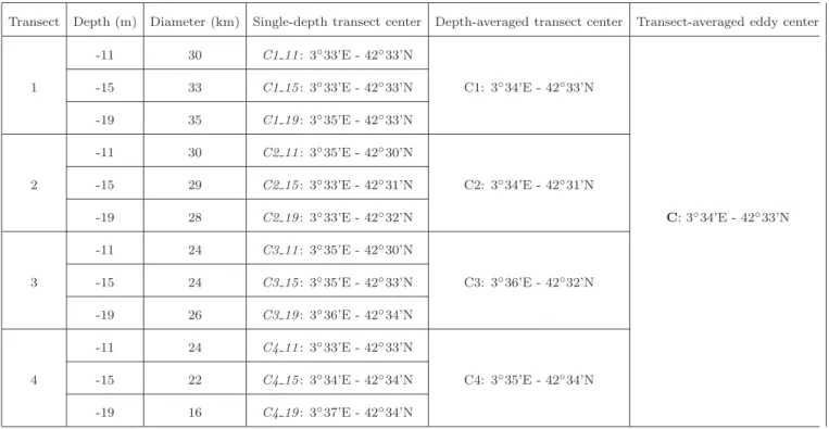
Table 2. Summary of the calculation of the position of the center of the eddy for each transect. The along transect diameter at the depth given in column 2 is provided in column 3.

Transect Depth (m) Diameter (km) Single-depth transect center Depth-averaged transect center Transect-averaged eddy center

-11 30 C1 11: 3◦_{33’E - 42}◦_33’N 1 -15 33 C1 15: 3◦_{33’E - 42}◦_{33’N C1: 3}◦_{34’E - 42}◦_33’N -19 35 C1 19: 3◦_{35’E - 42}◦_33’N -11 30 C2 11: 3◦_{35’E - 42}◦_30’N 2 -15 29 C2 15: 3◦_{33’E - 42}◦_{31’N C2: 3}◦_{34’E - 42}◦_31’N -19 28 C2 19: 3◦_{33’E - 42}◦_32’N C_{: 3}◦_{34’E - 42}◦_33’N -11 24 C3 11: 3◦_{35’E - 42}◦_30’N 3 -15 24 C3 15: 3◦_{35’E - 42}◦_{33’N C3: 3}◦_{36’E - 42}◦_32’N -19 26 C3 19: 3◦_{36’E - 42}◦_34’N -11 24 C4 11: 3◦_{33’E - 42}◦_33’N 4 -15 22 C4 15: 3◦_{34’E - 42}◦_{34’N C4: 3}◦_{35’E - 42}◦_34’N -19 16 C4 19: 3◦_{37’E - 42}◦_34’N

Gulf of Lion Catalan Sea Cape d’Agde FRANCE Cape Creus Marseille Roussillon Leucate

2

o

E

3

o

E

4

o

E

5

o

E

6

o

E

7

o

E

41

o

N

30’

42

o

N

30’

43

o

N

30’

44

o

N

30’

Longitude

Latitude

500

1000

1500

2000

2500

Figure 1. _{Model domain. The rectangle represents the model domain of 1 km × 1 km} resolution. Shaded color represents the bathymetry [m]. Isobaths at 100, 200 and 500 m are plotted with thin lines. The white arrow shows the mean position of the Northern Current (NC).

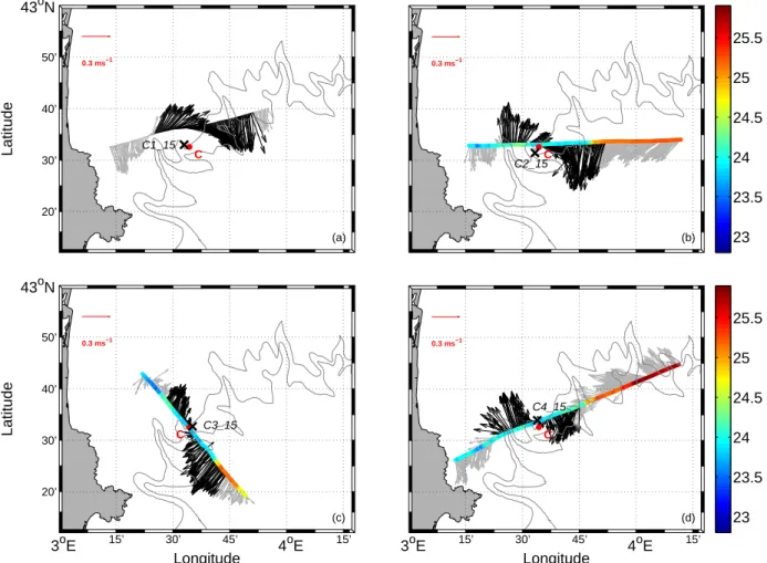
C1_15 C (a) Latitude 0.3 ms−1 20’ 30’ 40’ 50’ 43oN C2_15 C (b) 0.3 ms−1 23 23.5 24 24.5 25 25.5 C3_15 C (c) Longitude Latitude 0.3 ms−1 3oE 15’ 30’ 45’ 4oE 15’ 20’ 30’ 40’ 50’ 43oN C4_15 C (d) 0.3 ms−1 3oE 15’ 30’ 45’ 4oE 15’ Longitude 23 23.5 24 24.5 25 25.5

Figure 2. ADCP current vectors at 15m depth for Transect 1 (a), Transect 2 (b), Transect 3 (c) and Transect 4 (d). The colors on the transect represent the surface temperature data (◦_C)

acquired along the trajectory. For each transect, the single-depth transect center at 15 m depth (black cross) is defined as the point for which the mean tangential velocity computed from the velocity vectors in black is maximum. The red dot corresponds to the eddy center.

0

5

10

15

20

25

30

35

−0.4

−0.2

0

0.2

0.4

(a)

Tang. velocity [m.s

−1

]

0

5

10

15

20

25

30

35

23.5

24

24.5

25

25.5

(b)

Distance from the center [km]

Temperature [

o

C]

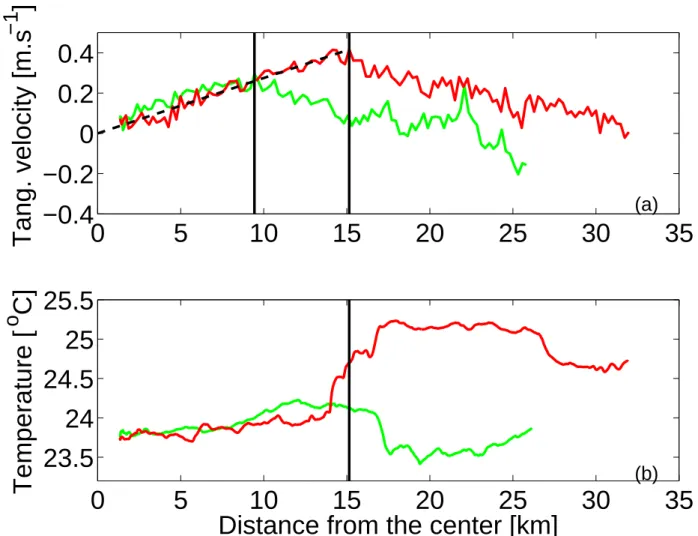
Figure 3. Distribution of tangential velocities at 15 m depth (a) and temperature at the surface (b) with respect to radial distance from C3 15. The green line corresponds to the data collected before crossing the center (hence northwest of the center C3 15 for Transect 3) and the red line corresponds to the data collected after the center (southeast of it). Black lines represent the distance from C3 15 where the maximum values of tangential velocities are reached. The black dashed line shows the linear increase of the tangential velocities in the case of a theoretical solid body rotation.

3oE 12’ 24’ 36’ 48’ 4oE 20’ 30’ 40’ 50’ 43oN 0.3 ms−1 (b) Longitude Latitude

Figure 4. (a) Vertical section (depth versus longitude) of the tangential component (clockwise, positive) of the horizontal currents [m s−1_{] for Transect 3. White pixels represent no data. ADCP}

current vectors at 27 m depth (b) for Transect 3. The black cross represent the single-depth transect center. The black circle represents the single-depth transect center at 27 m depth, common to figures a and b.

CTD_out CTD_edge CTD_in (a) 3oE 15’ 30’ 45’ 4oE 15’ 20’ 30’ 40’ 50’ 43oN Longitude Latitude 12 14 16 18 20 22 24 −160 −140 −120 −100 −80 −60 −40 −20 0 (b) Potential Temperature [ oC] Depth [m] CTD_out CTD_edge CTD_in 0 1 2 3 −160 −140 −120 −100 −80 −60 −40 −20 0 (c) Fluorescence [µg l−1] CTD_out CTD_edge CTD_in

Figure 5. (a) The three crosses represent the positions of the CTD stations (CTD in, CTD edge, CTD out). The blue circle is centered at the eddy center C (red dot) with a ra-dius equal to the one estimated for the eddy. Vertical profiles of potential temperature (b) and fluorescence (c) at three CTD stations on August 26 (CTD out: Outside part of the eddy located to the north; CTD edge: Northern edge of the eddy; CTD in: Inside part of the eddy).

2m/s 6m/s 10m/s 14m/s WEST EAST SOUTH NORTH (a) 2m/s 6m/s 10m/s 14m/s WEST EAST SOUTH NORTH (b) 2m/s 6m/s 10m/s 14m/s WEST EAST SOUTH NORTH (c) 2m/s 6m/s 10m/s 14m/s WEST EAST SOUTH NORTH (d) 0% 1−10% 10−20% 20−30% 0.3 ms−1 (e) 3oE 20’ 40’ 4oE 20’ 40’ 41oN 30’ 42oN 30’ 43oN 30’ Longitude Latitude 0.3 ms−1 (f) 3oE 20’ 40’ 4oE 20’ 40’ N 30’ N 30’ N 30’ Longitude Longitude 0.3 ms−1 (g) 3oE 20’ 40’ 4oE 20’ 40’ N 30’ N 30’ N 30’ 0.3 ms−1 (h) 3oE 20’ 40’ 4oE 20’ 40’ N 30’ N 30’ N 30’ Longitude −0.2 −0.18 −0.16 −0.14 −0.12 −0.1 −0.08 −0.06

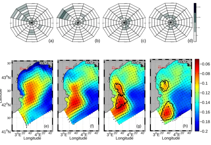
Figure 6. Time sequence of the generation process of A2-Latex09 in 2009. Top: wind rose representation (intensity and frequency) at station Leucate on (a) 2009/07/18 to 20; (b) 2009/08/06 to 08; (c) 2009/08/14 to 16; (d) 2009/08/25 to 27; colors representing wind frequency (%). Bottom: sea surface height [m] and current velocity field at 5 m depth on (e) 2009/07/20; (f) 2009/08/08; (g) 2009/08/16; (h) 2009/08/27. Black contours in (g) and (h) show the eddies identification issued from the wavelet analysis.

Figure 7. 3-dimensional sections of potential vorticity [kg m−4 _s−1_{] in color on September 3.}

The coast is represented in gray with the position of the Cape Creus. At 10 m depth, in the first section, we can distinguish the presence of A2-Latex09 upstream the Cape Creus. In the lee of the Cape, the transient structure is evidenced at 20 m depth. The Catalan eddy is also visualized farther off the coast and until 40 m depth.

0.3 ms−1 (a) 3oE 20’ 40’ 4oE 20’ 41oN 30’ 42oN 30’ 43oN Longitude Latitude −4 −3 −2 −1 0 1 2 3 4 x 10−5 (b)

3

E

4

E

41

N

42

N

43

N

Figure 8. (a) Modeled relative vorticity [s−1_{] and current velocity field at 20 m depth on}

September 3. (b) SSTb satellite image on August 28 (data from M´et´eo-France) and drifter

trajectories (drifter No. 83631 in blue - drifter No. 83632 in purple) from August 26 to September 12. The squares represent the drifters’ initial positions. The red dot corresponds to the eddy center.