HAL Id: hal-01919326
https://hal.univ-brest.fr/hal-01919326
Submitted on 18 Dec 2020
HAL is a multi-disciplinary open access
archive for the deposit and dissemination of
sci-entific research documents, whether they are
pub-lished or not. The documents may come from
teaching and research institutions in France or
abroad, or from public or private research centers.
L’archive ouverte pluridisciplinaire HAL, est
destinée au dépôt et à la diffusion de documents
scientifiques de niveau recherche, publiés ou non,
émanant des établissements d’enseignement et de
recherche français ou étrangers, des laboratoires
publics ou privés.
Distributed under a Creative Commons Attribution - NoDerivatives| 4.0 International
License
LiDAR Validation of a Video-Derived Beachface
Topography on a Tidal Flat
David Didier, Pascal Bernatchez, Emmanuel Augereau, Charles Caulet, Dany
Dumont, Eliott Bismuth, Louis Cormier, France Floc’h, Christophe Delacourt
To cite this version:
David Didier, Pascal Bernatchez, Emmanuel Augereau, Charles Caulet, Dany Dumont, et al.. LiDAR
Validation of a Video-Derived Beachface Topography on a Tidal Flat. Remote Sensing, MDPI, 2017,
9 (8), �10.3390/rs9080826�. �hal-01919326�
remote sensing
Article
LiDAR Validation of a Video-Derived Beachface
Topography on a Tidal Flat
David Didier1,*, Pascal Bernatchez1, Emmanuel Augereau2, Charles Caulet2,
Dany Dumont3 ID, Eliott Bismuth1, Louis Cormier1, France Floc’h2and Christophe Delacourt2 1 Québec-Océan, Centre d’études nordiques, Chaire de Recherche en Géoscience Côtière,
Université du Québec à Rimouski, Rimouski, QC G5L 3A1, Canada; [email protected] (P.B.); [email protected] (E.B.); [email protected] (L.C.)
2 Laboratoire Géosciences Océan UMR 6538, Institut Universitaire Européen de la mer, Université de Bretagne Occidentale, Brest, 29280 Plouzané, France;
[email protected] (E.A.); [email protected] (C.C.); [email protected] (F.F.); [email protected] (C.D.)
3 Institut des Sciences de la mer de Rimouski, Université du Québec à Rimouski, Québec-Océan,
Physique des Océans—Laboratoire de Rimouski, Rimouski, QC, G5L 3A1, Canada; [email protected]
* Correspondence: [email protected]; Tel.: +1-418-723-1986 (ext. 1364) Received: 26 June 2017; Accepted: 7 August 2017; Published: 11 August 2017
Abstract: Increasingly used shore-based video stations enable a high spatiotemporal frequency analysis of shoreline migration. Shoreline detection techniques combined with hydrodynamic conditions enable the creation of digital elevation models (DEMs). However, shoreline elevations are often estimated based on nearshore process empirical equations leading to uncertainties in video-based topography. To achieve high DEM correspondence between both techniques, we assessed video-derived DEMs against LiDAR surveys during low energy conditions. A newly installed video system on a tidal flat in the St. Lawrence Estuary, Atlantic Canada, served as a test case. Shorelines were automatically detected from time-averaged (TIMEX) images using color ratios in low energy conditions synchronously with mobile terrestrial LiDAR during two different surveys. Hydrodynamic (waves and tides) data were recorded in-situ, and established two different cases of water elevation models as a basis for shoreline elevations. DEMs were created and tested against LiDAR. Statistical analysis of shoreline elevations and migrations were made, and morphological variability was assessed between both surveys. Results indicate that the best shoreline elevation model includes both the significant wave height and the mean water level. Low energy conditions and in-situ hydrodynamic measurements made it possible to produce video-derived DEMs virtually as accurate as a LiDAR product, and therefore make an effective tool for coastal managers.
Keywords: video monitoring; shoreline detection; beach morphology; mobile terrestrial LiDAR; erosion; Atlantic Canada
1. Introduction
Beaches evolve through time and space, influenced by morphogenetic processes occurring in multiple dimensions in the surf and swash zones [1]. Following wave breaking, different short-term dynamic processes occur on a beach, mostly wave-induced high/low-frequency swash motions [2], groundwater/bed interactions [3,4], and scouring [5]. The beach morphology usually tends toward an equilibrium slope resulting from an onshore/offshore sediment transport induced by waves and currents [6–8]. Changes also occur on longer time scales where beaches are affected by strong seasonal cycles. For example, in cold regions, the presence of sea ice can protect (i.e., consolidates beach sediments) or erode (i.e., scouring at the icefoot’s toe, transport by drift ice, etc.) the beach profile [9].
Remote Sens. 2017, 9, 826 2 of 22
Multi-year analyses of the shoreline position can show variabilities on a kilometer scale on sandy coasts [10,11], while geologically constrained and protected systems like platform-beaches [12,13] and pocket-beaches [14] can show little changes. Capturing relevant morphogenic processes across different scales is not straightforward, namely because of the low temporal resolution of most monitoring strategies (large time interval between field campaigns) [10] that filter short-term events. Along with climate change and sea-level rise, beach morphodynamics can therefore be confusing and misunderstood by coastal managers and engineers in need of operational tools in order to deal with constantly evolving beaches [15]. On erosion hotspots [16], it is imperative to better understand the multi-scale variability of the beach morphology and slope, which are essential for flood risk assessment and to design protective structures in suitable adaptation strategies.
Out of many technological tools for beach morphology monitoring such as total stations [17], DGPS surveys [18–20], radar [21], UAV [22–24], or LiDAR [25–27], perhaps the shore-based video imagery is the most versatile. Such systems can be installed virtually everywhere for continuous recording over a long period of time [28], and are not directly vulnerable to extreme events as opposed to in-situ instruments [29]. In terms of spatiotemporal resolutions, video cameras offer other great perspectives, enabling both short-term and long-term monitoring capabilities. Video imagery is clearly effective for wave runup measurements, including swash and setup [30–33]. It then can be applied to calibrate empirical formulae in low and high energy situations through time-stack analysis [34,35]. Applied on video imagery, shoreline detection techniques based on time-exposure images can also acquire high-frequency topographical information when combined with hydrodynamic forcing [36–38]. With a relatively low cost [39], one can obtain digital elevation models (DEMs) with a few centimetres accuracy [37]. However, such systems and subsequent image analysis needs to be adapted to local conditions, since relationships between image optical characteristics and environmental/geometrical conditions on beaches are not always understood [40], especially in cold environments where coastal sea ice interferes with sediment dynamics [41].
A video-based shoreline evolution monitoring typically integrates two parameters: the shoreline detection and the water elevation model [42]. Swash and wave breaking on reflective beaches typically enhance beach/water pixel gradient intensities, seen as foamy bright bands, facilitating its detection using grey-scale images [43,44]. However, detecting shorelines on dissipative beaches with large surf zones is not as straightforward since the cross-shore pixel intensities/variance due to waves and foam motions [38] is scattered along a larger area. Another problem arises in enclosed areas with less energetic conditions such as estuaries [45], or on the landward side of sandbars [37]. To avoid these problems, some authors have proposed shoreline detection techniques based on full color characteristics of the imagery, especially using ARGUS stations [42,46], as opposed to traditional grey-scale image analysis developed earlier [43]. Almar et al. [37] also detected shorelines based on color analysis, but added a correction due to alongshore swash shapes at different tidal levels to estimate the intertidal topography at a double-barred and energetic meso-tidal beach in Biscarrose, France. The resulting morphology performed well with GPS validation runs for low energetic conditions (significant wave height, Hs< 1 m). Detected planimetric shorelines can be compared to
GPS runs on the beach at the time of the detection, with horizontal uncertainties generally varying between ~1 and 6 m [42,45,47].
The water elevation associated with a detected shoreline commonly includes the still water level (astronomical tide plus the barometric surge), and wave-induced runup (including setup and swash) [10,37,47,48]. The former component, the offshore static water level, is mostly known with in-situ gauge prior wave breaking. The latter is more complicated to obtain, since foreshore dynamics are most notably deduced with empirical formulations. Aarninkhof et al. [42] computed the setup and swash oscillation elevations, and concluded that their technique detected a shoreline at the upper end of the swash runup. Apart from uncertainties in planimetric shoreline detections and inherent to RTK-GPS validations and ground control points, these techniques imply uncertainties associated with the empirical formulations used. Such equations are limited to the input conditions only, and
Remote Sens. 2017, 9, 826 3 of 22
common vertical errors and deviations between theoretical results and observed values can range from 0.5 to 2 m [13,49,50]. In estuaries with mudflats, Morris et al. [45] used RTK-DGPS to validate video-derived shoreline elevations and obtained vertical errors within 5 cm. On more open coasts with moderate to high energy conditions, Vousdoukas et al. [47], Uunk et al. [36], and Aarninkhof et al. [42] also found low elevation error values using field DGPS validations, respectively of 26 cm, 28 cm, and 15 cm. Subsequent associations of detected shorelines with empirical formulations seems to show good results in most cases, but local validations appear to be necessary both for detected shorelines and the associated water levels. In low-energy environments such as estuaries and sandflats, the absence of significantly contrasting swash on the beach motivated this study.
Beaches along the St. Lawrence maritime Estuary (Atlantic Canada) typically show such characteristics. Furthermore, in such cold environments, the progressive disappearance of coastal sea ice during winter due to climate change leads to an enhancement of coastal erosion [51]. In order to analyze these multi-scale dynamics, efficient methodology to retrieve shoreline evolution is needed. This paper aims to create digital elevations models based on image-detected shorelines and to validate the video-derived topography on a low-energy meso-tidal beachface with a two-kilometer-wide sandflat. The shoreline elevations are obtained with in-situ wave and tidal gauges landward of the surf zone. Resulting digital elevation models are compared to simultaneous mobile LiDAR acquisition results. The LiDAR-interpolated topography acts as a validation tool for the video-based topography. Finally, the shoreline displacement rates during the autumn of 2016 are calculated from both video and LiDAR-based topography in order to compare both methods.
2. Materials and Methods 2.1. Study Area
The Manicouagan Peninsula is located on the north shore of the St. Lawrence maritime Estuary (Figure1). This imposing delta was formed in the Goldthwait Sea during the last deglaciation. During the Laurentian transgression which ended around 4.4–4.2 ka years BP, an important erosion platform was carved in the fine prodeltaic sediments, forming today steep beachfaces over a sandy flat as wide as 2 km in the cross-shore direction [52].
Despite previous Quaternary [52–54], coastal erosion [51], and sea ice [55,56] studies in the area, little is known on the morphodynamics of the Manicouagan beaches. Coastal citizens are facing constant erosion and one of the hotspots is located on the beach of Pointe-Lebel (Figure 1c). Shrinking winter sea ice and its predicted disappearance in the second half of the 21st century [55,56] will potentially increase erosion problems during the cold season by enabling storm waves to reach the beach. Deposited beach materials in Pointe-Lebel consist mainly of coarse and medium sands coming from sedimentary coastal cliffs. Beach erosion reached around−1.2 m and
−2.9 m/year (1931–2001) [51].
Tides around the Manicouagan Peninsula are semi-diurnal and meso-tidal, ranging between 3 and 4.3 m, and reaching up to 4.9 m during extreme spring tides [57], with currents reaching 3 m/s [58]. All tidal levels will be subsequently referred to their local geodetical datum (CGVD28), according to a difference of−1.81 m with the chart datum (mean sea levels (MSL) = 0 m; chart datum (CD) = −1.81 m; Higher high water large tide (HHWLT) = 2.89 m; Lower low water large tide (LLWLT) =−1.19 m). The Pointe-Lebel beach studied in this paper is characterized by a low-tide terrace/non-barred dissipative shape (considering the Masselink and Short [59] and Scott et al. [60] classifications). It is bounded by two small creeks forming deltas on the lower foreshore (see Figure1c). The main longshore drift is oriented toward northeast [52]. The wide intertidal sandflat is covered in some places with sandy accumulation banks of low amplitude. At high tide, swash occurs on a more reflective beachface with an average width of 20 m. The beachface is delimited on its upper part by an erosion scarp and on its lower limit by a hinge line. This break of slope marks the beginning of the lower foreshore which stretches over more than 2 km at low tide.
Remote Sens. 2017, 9, 826 4 of 22
Remote Sens. 2017, 9, 826 4 of 22
Figure 1. Location of the Manicouagan Peninsula (a,b) and of the monitoring station at Pointe-Lebel
(c). Two video cameras are installed with 2 instruments (G1: nearshore pressure sensor logger; G2: offshore acoustic, wave and current meter (AWAC) for in-situ hydrodynamic acquisition (black circles) (b,c)).
The offshore wave climate is mainly generated from dominant westerlies and strong easterly winds [61]. Beaches of the Manicouagan Peninsula can be exposed to strong ENE winds blowing on a 350 km long fetch [53]. Being oriented ESE, this is especially the case of the Pointe-Lebel beach where the video camera system is located. Ruest et al. [56] simulated wave heights with winds from the Modern-Era Retrospective Analysis for Research and Applications (MERRA) re-analysis in the Estuary. Simulated extreme waves (99th percentile Hs) are between 1 and 2 m, while the 50-year
return Hs is higher (between 2.5 and 4 m) for the whole Estuary. As per the authors, wave heights in
the Gulf of St. Lawrence are going to increase by 5–10% by 2100 with extensive ice-free periods during winter.
2.2. Wave and Tidal Data
Waves were measured with an array of two in-situ gauges between 1 July 2016 and 30 December 2016 (Figure 2). The first sensor (RBR Virtuoso) is located at the toe of the beachface close to the break in the foreshore slope (G1, z = 0.20 m), landward of the tidal flat. This nearshore sensor acquired continuous total pressures at a 4 Hz frequency, and was subsequently processed through a spectral analysis over a length of 1024 s (17.06 min). Offshore waves were acquired at 2 Hz with an Acoustic Wave and Current meter (AWAC) deployed at 14 m depth (G2) (Figure 2b) southeast of
Figure 1.Location of the Manicouagan Peninsula (a,b) and of the monitoring station at Pointe-Lebel (c). Two video cameras are installed with 2 instruments (G1: nearshore pressure sensor logger; G2: offshore acoustic, wave and current meter (AWAC) for in-situ hydrodynamic acquisition (black circles) (b,c)).
The offshore wave climate is mainly generated from dominant westerlies and strong easterly winds [61]. Beaches of the Manicouagan Peninsula can be exposed to strong ENE winds blowing on a 350 km long fetch [53]. Being oriented ESE, this is especially the case of the Pointe-Lebel beach where the video camera system is located. Ruest et al. [56] simulated wave heights with winds from the Modern-Era Retrospective Analysis for Research and Applications (MERRA) re-analysis in the Estuary. Simulated extreme waves (99th percentile Hs) are between 1 and 2 m, while the 50-year
return Hsis higher (between 2.5 and 4 m) for the whole Estuary. As per the authors, wave heights
in the Gulf of St. Lawrence are going to increase by 5–10% by 2100 with extensive ice-free periods during winter.
2.2. Wave and Tidal Data
Waves were measured with an array of two in-situ gauges between 1 July 2016 and 30 December 2016 (Figure2). The first sensor (RBR Virtuoso) is located at the toe of the beachface close to the break in the foreshore slope (G1, z = 0.20 m), landward of the tidal flat. This nearshore sensor acquired continuous total pressures at a 4 Hz frequency, and was subsequently processed through a spectral
Remote Sens. 2017, 9, 826 5 of 22
analysis over a length of 1024 s (17.06 min). Offshore waves were acquired at 2 Hz with an Acoustic Wave and Current meter (AWAC) deployed at 14 m depth (G2) (Figure2b) southeast of Pointe-Lebel. The cross-shore distance of both instruments from the HHWLT line on the beach is respectively 23 m and 4.5 km offshore. Calculated spectral wave parameters are the significant wave height (Hs),
mean periods (Tm02), and offshore mean wave directions θ at G2. Atmospheric pressure was obtained
from a barometric pressure gauge (HOBO data logger) every 10 min and interpolated to wave sampling rates. Mean water level (η) was calculated from mean pressure on both instruments.
Remote Sens. 2017, 9, 826 5 of 22
Pointe-Lebel. The cross-shore distance of both instruments from the HHWLT line on the beach is respectively 23 m and 4.5 km offshore. Calculated spectral wave parameters are the significant wave height (Hs), mean periods (Tm02), and offshore mean wave directions θ at G2. Atmospheric pressure
was obtained from a barometric pressure gauge (HOBO data logger) every 10 min and interpolated to wave sampling rates. Mean water level (η) was calculated from mean pressure on both instruments.
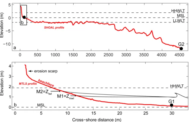
Figure 2. Cross-shore profile (extracted from a shoal survey of 2015 obtain from the Canadian
Hydrographic Service, 2015) of Pointe-Lebel beach and location of the in-situ instruments (G1 and G2) (a). A focus on the beachface is shown in (b) from the MTLS (Mobile Terrestrial Lidar System) survey of 3 August 2016. Elevations associated to higher high water large tides (HHWLT), mean sea levels (MSL) and lower low water large tides (LLWLT) are shown by horizontal dashed lines.
Mean water level fluctuations recorded offshore during the entire joint deployment period oscillated between −2.42 and 3.17 m. The sensor G1 recorded a maximum Hs of 0.98 m on 16
November 2016. During the LiDAR surveys of 3 August and 18 November (vertical lines on Figure 3), the conditions were calm and the maximum mean water levels at G1 reached 1.48 m and 2.25 m at high tide, respectively. Significant wave heights did not exceed 0.14 m during the surveys.
Figure 2. Cross-shore profile (extracted from a shoal survey of 2015 obtain from the Canadian Hydrographic Service, 2015) of Pointe-Lebel beach and location of the in-situ instruments (G1 and G2) (a). A focus on the beachface is shown in (b) from the MTLS (Mobile Terrestrial Lidar System) survey of 3 August 2016. Elevations associated to higher high water large tides (HHWLT), mean sea levels (MSL) and lower low water large tides (LLWLT) are shown by horizontal dashed lines.
Mean water level fluctuations recorded offshore during the entire joint deployment period oscillated between −2.42 and 3.17 m. The sensor G1 recorded a maximum Hs of 0.98 m on
16 November 2016. During the LiDAR surveys of 3 August and 18 November (vertical lines on Figure3), the conditions were calm and the maximum mean water levels at G1 reached 1.48 m and 2.25 m at high tide, respectively. Significant wave heights did not exceed 0.14 m during the surveys.
Remote Sens. 2017, 9, 826 6 of 22
Remote Sens. 2017, 9, 826 6 of 22
Figure 3. Mean water level (with daily tidal cycles) (m) (a), significant wave height (m) (b), mean
wave direction (°) (c), and period (s) (d) recorded between July and December 2016. The surveys of 3 August and 18 November 2016 are shown by vertical grey bands.
During the autumn of 2016 (September to December), more energetic events were observed. Offshore significant wave heights reached a maximum of 3.8 m at G2 on 12 November, but it happened at low tide and dissipation across the tidal flat prevented incoming waves to reach the beach. On 16 November, waves at the beachface toe reached 0.92 m, and mean wave directions (observed offshore) spanned between 99° and 123° (ESE) throughout the day.
2.3. LiDAR Survey and Topographic Data
A Mobile Terrestrial LiDAR System (MTLS), hereinafter referred to as LiDAR, was used to acquire a high-resolution beach topography on 3 August 2016 (Figure 4) and 18 November 2016. Both surveys were conducted at low tide. The LiDAR is mounted on a utility side by side vehicle (Figure 5b) moving at ~30–40 km/h. The system includes a laser scanner Riegl VQ-250 and a GPS inertial navigation system Applanix POS-LV 220. Post-processing for raw data analysis is described in Didier et al. [62]. A manual filtering of the debris on the beach was made on the raw LiDAR data (dense point cloud) to delete trees and driftwood from the final LiDAR topography. The RMS errors (x, y, z) (23 control points) between RTK-GPS (Trimble R8) and adjacent laser points was assessed in Didier et al. [62] and are in the order ±0.03 m [62]. The LiDAR data were used as a validation surface for each detected and orthorectified shoreline.
Figure 3.Mean water level (with daily tidal cycles) (m) (a), significant wave height (m) (b), mean wave direction (◦) (c), and period (s) (d) recorded between July and December 2016. The surveys of 3 August and 18 November 2016 are shown by vertical grey bands.
During the autumn of 2016 (September to December), more energetic events were observed. Offshore significant wave heights reached a maximum of 3.8 m at G2 on 12 November, but it happened at low tide and dissipation across the tidal flat prevented incoming waves to reach the beach. On 16 November, waves at the beachface toe reached 0.92 m, and mean wave directions (observed offshore) spanned between 99◦and 123◦(ESE) throughout the day.
2.3. LiDAR Survey and Topographic Data
A Mobile Terrestrial LiDAR System (MTLS), hereinafter referred to as LiDAR, was used to acquire a high-resolution beach topography on 3 August 2016 (Figure4) and 18 November 2016. Both surveys were conducted at low tide. The LiDAR is mounted on a utility side by side vehicle (Figure5b) moving at ~30–40 km/h. The system includes a laser scanner Riegl VQ-250 and a GPS inertial navigation system Applanix POS-LV 220. Post-processing for raw data analysis is described in Didier et al. [62]. A manual filtering of the debris on the beach was made on the raw LiDAR data (dense point cloud) to delete trees and driftwood from the final LiDAR topography. The RMS errors (x, y, z) (23 control points) between RTK-GPS (Trimble R8) and adjacent laser points was assessed in Didier et al. [62] and are in the order±0.03 m [62]. The LiDAR data were used as a validation surface for each detected and orthorectified shoreline.
Remote Sens. 2017, 9, 826 7 of 22
Remote Sens. 2017, 9, 826 7 of 22
Figure 4. LiDAR point cloud from the survey of 3 August 2016 on the beach of Pointe-Lebel shown in
aerial (a) and perspective (b) views. 2.4. Video Monitoring Station
The beach of Pointe-Lebel was equipped with two AXIS P3367-VE video camera systems on 8 June 2016 (Figures 4b and 5). Both cameras are installed on a pole originally located at 5 m from the beach (49.092°N, 68.227°W). The system is directly connected to a power grid. Each camera covers a pan range of 84° and a shadow zone varying from ~1 m near the system to ~10 m at the beachface toe is located between both camera views (no overlap between views). The total view reaches ~180°. Cameras are precisely located at 12.08 m above the mean sea level and offer a continuous sampling acquisition of 4 Hz (2592 × 1944 pixels, 5 megapixels) during daylight (~10 h/day). Both Power Over the Ethernet (POE) IP cameras are accessible online for remote modifications via a 4G network, and are connected on a laptop computer (Lenovo Intel® Core™ i5-6200 U CPU, 2.3 GHz–2.4 GHz, 8 Go
RAM, 64 bits) located in a sealed box on the system post. All videos are recorded directly on physical hard drives to assure and secure data acquisition during all weather conditions, particularly during winter.
Figure 4.LiDAR point cloud from the survey of 3 August 2016 on the beach of Pointe-Lebel shown in aerial (a) and perspective (b) views.
2.4. Video Monitoring Station
The beach of Pointe-Lebel was equipped with two AXIS P3367-VE video camera systems on 8 June 2016 (Figures4b and5). Both cameras are installed on a pole originally located at 5 m from the beach (49.092◦N, 68.227◦W). The system is directly connected to a power grid. Each camera covers a pan range of 84◦and a shadow zone varying from ~1 m near the system to ~10 m at the beachface toe is located between both camera views (no overlap between views). The total view reaches ~180◦. Cameras are precisely located at 12.08 m above the mean sea level and offer a continuous sampling acquisition of 4 Hz (2592×1944 pixels, 5 megapixels) during daylight (~10 h/day). Both Power Over the Ethernet (POE) IP cameras are accessible online for remote modifications via a 4G network, and are connected on a laptop computer (Lenovo Intel®Core™ i5-6200 U CPU, 2.3 GHz–2.4 GHz, 8 Go RAM, 64 bits) located in a sealed box on the system post. All videos are recorded directly on physical hard drives to assure and secure data acquisition during all weather conditions, particularly during winter.
Remote Sens. 2017, 9, 826 8 of 22
Remote Sens. 2017, 9, 826 8 of 22
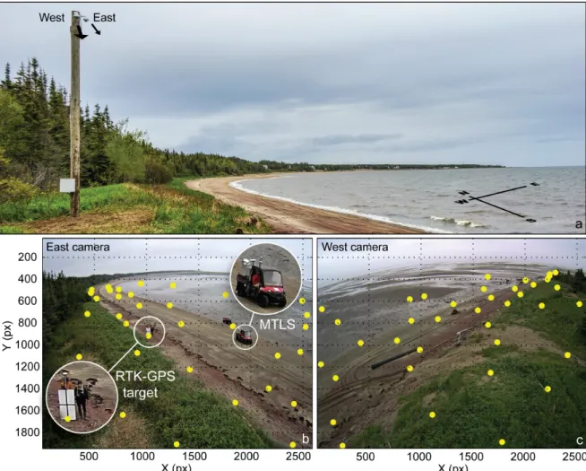
Figure 5. The video camera system of Pointe-Lebel is located at 5 m from the beachface (a). Ground
Control Points (GCPs showed as yellow dots) for image to ground coordinate conversions were acquired with RTK–GPS on the beachface and the tidal flat during the LiDAR survey on the east (b) and west side of the beach (c) on 3 August 2016. The GCPs and LiDAR acquisitions are shown in (b). 2.5. Cameras Calibration
Optical measurements are subject to image distortions due to inherent camera characteristics. The calibration process enables an estimation of these parameters, and establishes a mapping conversion model from image to ground coordinates. The technique described in Stumpf et al. [63] was used because of its ability to deal with radial lens distortion and estimations for exterior orientation, focal length, skew factor, and principal point. The calibration requires at least nine ground control points (GCPs) for each camera that cover the entire camera view and that are evenly distributed on the beach and tidal flat at low tide. Only GCPs closer than 230 m from the camera system (yellow dots in Figure 5b,c, east: 33 GCPs; west: 38 GCPs) were used for the calibration in order to minimize the horizontal uncertainty, resulting to final GCP RMSEs of 0.38 and 1.11 m for the west and east cameras, respectively. The mapping algorithm was then used to convert all detected shorelines (pixel coordinates) into ground coordinates.
The alongshore pixel footprint increases with distance from the cameras. Within 230 m, projections of each pixel from camera dimensions to x-y geographical coordinates result in ground pixel footprints of 1 cm × 1 cm (longshore × cross-shore) close to the cameras. It increases up to 2.8 m in the alongshore direction while the cross-shore footprint remains under 0.5 m.
2.6. Shoreline Detection and Water Elevation Models
Five-minute video segments were acquired during the rising tide of 3 August 2016 between 12:50 and 16:00 (EST) and on 18 November 2016 between 14:00 and 17:30 (EST). LiDAR surveys were
Figure 5.The video camera system of Pointe-Lebel is located at 5 m from the beachface (a). Ground Control Points (GCPs showed as yellow dots) for image to ground coordinate conversions were acquired with RTK–GPS on the beachface and the tidal flat during the LiDAR survey on the east (b) and west side of the beach (c) on 3 August 2016. The GCPs and LiDAR acquisitions are shown in (b). 2.5. Cameras Calibration
Optical measurements are subject to image distortions due to inherent camera characteristics. The calibration process enables an estimation of these parameters, and establishes a mapping conversion model from image to ground coordinates. The technique described in Stumpf et al. [63] was used because of its ability to deal with radial lens distortion and estimations for exterior orientation, focal length, skew factor, and principal point. The calibration requires at least nine ground control points (GCPs) for each camera that cover the entire camera view and that are evenly distributed on the beach and tidal flat at low tide. Only GCPs closer than 230 m from the camera system (yellow dots in Figure5b,c, east: 33 GCPs; west: 38 GCPs) were used for the calibration in order to minimize the horizontal uncertainty, resulting to final GCP RMSEs of 0.38 and 1.11 m for the west and east cameras, respectively. The mapping algorithm was then used to convert all detected shorelines (pixel coordinates) into ground coordinates.
The alongshore pixel footprint increases with distance from the cameras. Within 230 m, projections of each pixel from camera dimensions to x-y geographical coordinates result in ground pixel footprints of 1 cm×1 cm (longshore×cross-shore) close to the cameras. It increases up to 2.8 m in the alongshore direction while the cross-shore footprint remains under 0.5 m.
Remote Sens. 2017, 9, 826 9 of 22
2.6. Shoreline Detection and Water Elevation Models
Five-minute video segments were acquired during the rising tide of 3 August 2016 between 12:50 and 16:00 (EST) and on 18 November 2016 between 14:00 and 17:30 (EST). LiDAR surveys were conducted simultaneously with video acquisitions. All image analyses were performed using Matlab. Outputs are 5-min time-averaged images (TIMEX) used for shoreline detections based on the presence of swash at the water/beach junction.
The shoreline detection is applied in two steps [38]. As a first approximation, all shorelines were automatically extracted based on a blue, green and red color ratio (B + G/R) on all TIMEX images, where B, G, and R are respectively the pixel intensity values of the blue, green, and red channels. The processing was computed for all pixels in a pre-defined region of interest (ROI) on the beach (Figure6a). The shoreline represents a local minimum in B + G/R ratios over the entire ROI, with lower ratio values (pixel ratio values <1) corresponding to the beachface while the water surface falls under higher ratios, typically over 1. The next step is the shoreline detection and identification on the TIMEX images. The technique is based on the alongshore shape of the swash on the beach in the ROI and detects the water/land boundary rather than dry/wet sand contours [38]. Falsely detected shorelines due to sunshine reflectance on the water, debris at the shoreline, and people on the beach were discarded, but no manual intervention was applied in the delineation.
Remote Sens. 2017, 9, 826 9 of 22
conducted simultaneously with video acquisitions. All image analyses were performed using Matlab. Outputs are 5-min time-averaged images (TIMEX) used for shoreline detections based on the presence of swash at the water/beach junction.
The shoreline detection is applied in two steps [38]. As a first approximation, all shorelines were automatically extracted based on a blue, green and red color ratio (B + G/R) on all TIMEX images, where B, G, and R are respectively the pixel intensity values of the blue, green, and red channels. The processing was computed for all pixels in a pre-defined region of interest (ROI) on the beach (Figure 6a). The shoreline represents a local minimum in B + G/R ratios over the entire ROI, with lower ratio values (pixel ratio values <1) corresponding to the beachface while the water surface falls under higher ratios, typically over 1. The next step is the shoreline detection and identification on the TIMEX images. The technique is based on the alongshore shape of the swash on the beach in the ROI and detects the water/land boundary rather than dry/wet sand contours [38]. Falsely detected shorelines due to sunshine reflectance on the water, debris at the shoreline, and people on the beach were discarded, but no manual intervention was applied in the delineation.
Figure 6. Time-averaged (TIMEX) image with a detected shoreline in calm conditions (red line) (a)
and geo-rectified detected shoreline (red line) shown on a time-averaged image from the east camera of Pointe-Lebel (b).
Figure 6.Time-averaged (TIMEX) image with a detected shoreline in calm conditions (red line) (a) and geo-rectified detected shoreline (red line) shown on a time-averaged image from the east camera of Pointe-Lebel (b).
Remote Sens. 2017, 9, 826 10 of 22
In order to create video-derived digital elevation models (DEMs) from all the image-detected shorelines, a constant alongshore elevation value was first attributed to each detected shoreline [64]. This step generally underlines some assumptions because knowing the exact shoreline elevation in the absence of in-situ water levels and wave time series is not straightforward. The association of water levels to shorelines is normally based on empirical formulations [65]. Here, two different water elevation models (referred to M1 and M2) were tested and associated to the detected shorelines to create two different video-based DEMs. Both water elevation models are associated to observed hydrodynamic parameters at G1 (at the beachface toe). The first model (M1), the image-detected shoreline elevation based on the mean water level Zmwl, is equal to ηtidewhich is the low-frequency
still water level (astronomical tide + barometric surge).
The second water elevation model (M2) represents the total water level (TWL) observed at the beach/water line junction (Ztwl). It includes the still water level and the wave effect through
the significant wave height. All analyses were made during low energy conditions to minimize uncertainties associated with high runup/setup values resulting from wave breaking [65,66]. Given that smaller waves are assumed to generate smaller runup values and therefore result in less detection errors due to swash length than during high energy conditions, the approach was applied during low energy conditions only (Hs< 0.15 m). M2 directly uses the nearshore observed significant wave
height instead of empirical runup equations based on offshore wave conditions that would obviously increase the overall uncertainty of the approach (e.g., [64,66]). The second model (M2) thus takes the following form:
Ztwl =ηtide+Hs (1)
The TWL model (M2) is justified by the fact that the Manicouagan peninsula mainly faces small waves outside of storm events, thus enabling the creation of DEMs with a high temporal resolution. We validated this assumption by extracting the occurrence associated to Hs < 0.15 m
from a WAVEWATCH III (WW3) simulation at 8.3 km offshore, eastward of the study site. WW3 is forced with atmospheric forcing from the Climate Forecast System Reanalysis (CFSR, NCEP/NOAA). Oceanic forcing (currents, water levels, sea ice thickness and concentration) come from a Regional Oceanic Model (ROM) (5 km×5 km grid) operated by the Institut des Sciences de la Mer de Rimouski (ISMER). Hourly waves were simulated for the 1980–2009 period at a 5-km grid. Considering the entire 30 yrs time series, offshore waves (Hs) are under 15 cm 58% of the time.
Errors associated with the video-based approach have been assessed. First, the LiDAR elevation associated to the detected shorelines was extracted to compare the overall effectiveness of both water elevation models (Zmwland Ztwl). This analysis enabled a direct comparison between the raw data
(image-detected shorelines elevations) and LiDAR points prior to the creation of DEMs. A TIN grid elevation was then created in LP360-QCoherent software from the LiDAR points and from both models of video-based contour lines (M1 and M2). Point clouds were all sampled to a fixed squared 20 cm×20 cm mesh grid. The latter was used to create the DEMs with the same pixel resolution of ∆x = ∆y = 20 cm. For both surveys, the overall surface elevation (z) of the LiDAR-derived matrices were compared to video-based DEMs with linear regression analysis.
The shoreline detection x–y errors were also analysed by extracting a reference contour line (rfl) associated to the mean high tide (z = 1.19) from all DEMs. This elevation was chosen because it is prone to be reached on the beach virtually every day, since it represents the mean level of high tides. The cross-shore variability of the rfl was systematically calculated at 5 m alongshore intervals between video-derived models and LiDAR within the same date. Furthermore, the performance of the video system to estimate the temporal shoreline cross-shore net displacements was analyzed. The cross-shore displacements of the rfl between November and August as observed with video cameras (∆yvid) were
compared to the displacements observed with the LiDAR system (∆ylid). Finally, in order to analyse
the potential of the video system to obtain morphological parameters on the beach in a context of risk management, beachface slopes tan βbf, particularly used in runup empirical equations [34] and
Remote Sens. 2017, 9, 826 11 of 22
zone. In this paper, tan βbfwas calculated between the maximum water level on the beach and the
beachface toe.
3. Results and Discussion
3.1. Shoreline Detection and Elevation Analyses
The video system provided continuous image acquisitions at 4 Hz during daylight on 3 August and 18 November 2016 on the beach of Pointe-Lebel. The image analysis was performed on 5-min TIMEX images during the rising tide while a pressure sensor located at the beach toe synchronously acquired mean water levels and wave characteristics. This setting enabled the extraction of 21 (~83,000 points) to 25 (~98,000 points) contour lines during 3 August and 18 November 2016, respectively. This difference is solely due to a larger tidal amplitude on November 18.
Most studies suggest using a longer averaging period, usually 10 min TIMEX [4,28,36,39,43,65,68] to 15 min [69]. The methodological choice of long period time-averaged images is based on the time period of wave groups and the fact that a longer exposure enables a more complete “storage” of the processes on the beach such as wave breaking [21] that generate foam at the shoreline or over bars. By recording all image intensities at each pixel during this period, commonly used detection techniques such as the SLIM (shoreline intensity maximum), ANN (artificial neural network), PIC (pixel intensity clustering) and CCD (color channel divergence) methods can be applied in most cases [48]. Using colour ratios combined with a pattern recognition algorithm does not necessarily require such long TIMEX durations as noted by Almar et al. [38]. In fact, using shorter time-averaged digital images (<2 min) can overcome some errors that could result from the local swash length on the beach. Although the sensitivity of the detection from varying image-averaging time was not assessed in this paper, 5 min-averaged shoreline detection was considered suitable for the rather steep beachface slope of Pointe-Lebel, thus minimizing possible errors that could arise from the tidal variation over the course of longer time-averaging period [48].
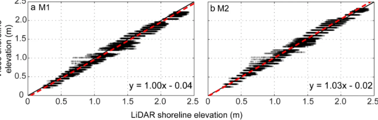
An assessment of the video-derived shoreline vertical accuracies was made. The correlation analysis between detected shoreline points and their correspondence on the LiDAR DEM shows that both shoreline elevation models perform well (Figure7). With vertical RMS errors of 0.06 m, and high correlation coefficients (R2= 0.99, p-value <0.001) (Table1), both linear regressions are well correlated.
Remote Sens. 2017, 9, 826 11 of 22
3. Results and Discussion
3.1. Shoreline Detection and Elevation Analyses
The video system provided continuous image acquisitions at 4 Hz during daylight on 3 August and 18 November 2016 on the beach of Pointe-Lebel. The image analysis was performed on 5-min TIMEX images during the rising tide while a pressure sensor located at the beach toe synchronously acquired mean water levels and wave characteristics. This setting enabled the extraction of 21 (~83,000 points) to 25 (~98,000 points) contour lines during 3 August and 18 November 2016, respectively. This difference is solely due to a larger tidal amplitude on November 18.
Most studies suggest using a longer averaging period, usually 10 min TIMEX [4,28,36,39,43,65,68] to 15 min [69]. The methodological choice of long period time-averaged images is based on the time period of wave groups and the fact that a longer exposure enables a more complete “storage” of the processes on the beach such as wave breaking [21] that generate foam at the shoreline or over bars. By recording all image intensities at each pixel during this period, commonly used detection techniques such as the SLIM (shoreline intensity maximum), ANN (artificial neural network), PIC (pixel intensity clustering) and CCD (color channel divergence) methods can be applied in most cases [48]. Using colour ratios combined with a pattern recognition algorithm does not necessarily require such long TIMEX durations as noted by Almar et al. [38]. In fact, using shorter time-averaged digital images (<2 min) can overcome some errors that could result from the local swash length on the beach. Although the sensitivity of the detection from varying image-averaging time was not assessed in this paper, 5 min-averaged shoreline detection was considered suitable for the rather steep beachface slope of Pointe-Lebel, thus minimizing possible errors that could arise from the tidal variation over the course of longer time-averaging period [48]. An assessment of the video-derived shoreline vertical accuracies was made. The correlation analysis between detected shoreline points and their correspondence on the LiDAR DEM shows that both shoreline elevation models perform well (Figure 7). With vertical RMS errors of 0.06 m, and high correlation coefficients (R2 = 0.99, p-value <0.001) (Table 1), both linear regressions are well
correlated.
Figure 7. Video-based shoreline elevations versus LiDAR data as parameterized with the shoreline
elevation model including only the mean water level (M1) (a) and the total water level (M2) (b). Regression lines are shown by red dashed lines. The black line represents the 1:1 line.
Differences lay mostly on the offset values, with an origin offset of −0.04 for the M1 (mean water level only) and −0.02 m for M2 (total water level), respectively. These results indicate that the overall contribution from Hs is small in the total water level approximation (M2) but it reduces the origin
offset by 2 cm. Slopes of both regression lines are very near 1:1, with the coefficient of the M2 being slightly higher than the M1 (1.03 instead of 1.00). Although the highest wave reached only 0.14 m, this difference can be mainly explained by higher waves at high tide in the M2 model, which is not considered in the mean water level model (M1). Almar et al. [38] noted similar results, indicating a positive and linear relationship between the detection errors and the local swash length, which in
Figure 7.Video-based shoreline elevations versus LiDAR data as parameterized with the shoreline elevation model including only the mean water level (M1) (a) and the total water level (M2) (b). Regression lines are shown by red dashed lines. The black line represents the 1:1 line.
Differences lay mostly on the offset values, with an origin offset of−0.04 for the M1 (mean water level only) and−0.02 m for M2 (total water level), respectively. These results indicate that the overall contribution from Hsis small in the total water level approximation (M2) but it reduces the origin
Remote Sens. 2017, 9, 826 12 of 22
slightly higher than the M1 (1.03 instead of 1.00). Although the highest wave reached only 0.14 m, this difference can be mainly explained by higher waves at high tide in the M2 model, which is not considered in the mean water level model (M1). Almar et al. [38] noted similar results, indicating a positive and linear relationship between the detection errors and the local swash length, which in return could necessitate a correction factor to reduce uncertainties associated with runup excursions [48]. This suggests that despite a lower origin offset in M2, using the mean water level only (M1) could potentially limit the uncertainty associated with higher wave heights at the beach. Moreover, the slope coefficient of the regression line being precisely 1.00 in M1 suggests that using mean water levels only during low wave conditions provides skillful results along the coast of Pointe-Lebel, as also noted by Morris et al. [45] in calm conditions on a tidal flat.
3.2. Comparing Video- to LiDAR-Based Topography
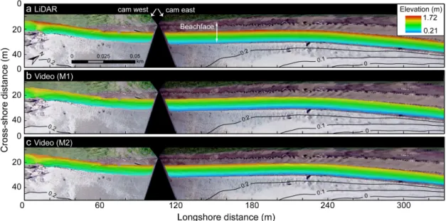
Digital elevation models were created from video-detected shorelines and LiDAR cloud points on the same 20 cm×20 cm meshgrid for both surveys. Both shoreline elevation models (from video) performed well in predicting the beachface shoreline elevations (Figure7), and such correspondence is also found on the resulting DEMs (results from August are shown as an example, Figure8). With the integration of Hsand the mean water level, M2 offers a more accurate morphology of the beachface
compared to M1. The sediment accumulation on the west part of the beach, clearly visible with the LiDAR survey, is more perceived with M2 although it is still present on the DEM produced with M1. Differences between video- and LiDAR-based topography were calculated to obtain a differential DEM in the ROI (Figures9and10). As shown in Figure9a,b, the sediment accumulation on the west part of the beach is explained by anthropogenic debris (hard plastic pipe drain) acting as an artificial tombolo. The reference line of the mean high tides (z = 1.19 m) was extracted from the 3 August survey (from each raster) and is presented to give an overview of the erosion that occurred between the surveys.
Remote Sens. 2017, 9, 826 12 of 22
return could necessitate a correction factor to reduce uncertainties associated with runup excursions[48]. This suggests that despite a lower origin offset in M2, using the mean water level only (M1) could potentially limit the uncertainty associated with higher wave heights at the beach. Moreover, the slope coefficient of the regression line being precisely 1.00 in M1 suggests that using mean water levels only during low wave conditions provides skillful results along the coast of Pointe-Lebel, as also noted by Morris et al. [45] in calm conditions on a tidal flat.
3.2. Comparing Video- to LiDAR-Based Topography
Digital elevation models were created from video-detected shorelines and LiDAR cloud points on the same 20 cm × 20 cm meshgrid for both surveys. Both shoreline elevation models (from video) performed well in predicting the beachface shoreline elevations (Figure 7), and such correspondence is also found on the resulting DEMs (results from August are shown as an example, Figure 8). With the integration of Hs and the mean water level, M2 offers a more accurate morphology of the
beachface compared to M1. The sediment accumulation on the west part of the beach, clearly visible with the LiDAR survey, is more perceived with M2 although it is still present on the DEM produced with M1. Differences between video- and LiDAR-based topography were calculated to obtain a differential DEM in the ROI (Figures 9 and 10). As shown in Figure 9a,b, the sediment accumulation on the west part of the beach is explained by anthropogenic debris (hard plastic pipe drain) acting as an artificial tombolo. The reference line of the mean high tides (z = 1.19 m) was extracted from the 3 August survey (from each raster) and is presented to give an overview of the erosion that occurred between the surveys.
Figure 8. Beachface topography of 3 August 2016 obtained from LiDAR (a) and video imagery as defined with (b) the shoreline elevation model 1 (M1, Zmwl) and (c) model 2 (M2, Ztwl).
Figure 8. Beachface topography of 3 August 2016 obtained from LiDAR (a) and video imagery as defined with (b) the shoreline elevation model 1 (M1, Zmwl) and (c) model 2 (M2, Ztwl).
Remote Sens. 2017, 9, 826 13 of 22
Remote Sens. 2017, 9, 826 13 of 22
Figure 9. Overall differences between the LiDAR surveys and the video-based topography for 3 August (a,b) and 18 November (c,d). The 1.19 m rfl of 3 August as extracted from the LiDAR is shown on all figures.
Figure 10. Relative frequency (%) of the Δ LiDAR-Zmwl (M1) and Δ LiDAR-Ztwl (M2) digital elevation
models’ (DEMs) differences (over all pixels) as observed during 3 August (a) and 18 November (b). Positive values indicate higher elevations on the LiDAR and underestimations by the shoreline detection model.
The sediment accumulation located on the west camera view (left side of Figure 9a,b) creates a shadow zone preventing the west camera to precisely locate the shorelines. This promotes rogue detections and therefore increased elevation uncertainties at this location. On Figure 9c,d, this sediment accumulation is no longer in place due to the beach’s response to a storm event that occurred on 16 November. As a result of sediment transport, the video-derived topography at this location is well predicted in November (Figure 9c,d).
The cameras in Pointe-Lebel being located at only 12 m above mean sea level, all analyses are limited to 230 m from each camera to keep planimetric errors lower than ~1 m. Within this distance, despite the shadow zone mentioned above, overall video-derived DEM elevation differences all range between −0.25 m and 0.29 m. Spatial coverage depends on the camera elevation [21]. These errors could therefore be overcome by elevating the cameras, as in previous works (e.g., McCarrol et al. [70] (55 m), Bracs et al. [65] (44 m), Sénéchal et al. [32], Almar et al. [38] (27 m), Vousdoukas et al. [47] (20 m), Abessolo Ondoa et al. [69] (15 m)).
Figure 9.Overall differences between the LiDAR surveys and the video-based topography for 3 August (a,b) and 18 November (c,d). The 1.19 m rfl of 3 August as extracted from the LiDAR is shown on all figures.
Remote Sens. 2017, 9, 826 13 of 22
Figure 9. Overall differences between the LiDAR surveys and the video-based topography for 3
August (a,b) and 18 November (c,d). The 1.19 m rfl of 3 August as extracted from the LiDAR is shown on all figures.
Figure 10. Relative frequency (%) of the Δ LiDAR-Zmwl (M1) and Δ LiDAR-Ztwl (M2) digital elevation
models’ (DEMs) differences (over all pixels) as observed during 3 August (a) and 18 November (b). Positive values indicate higher elevations on the LiDAR and underestimations by the shoreline detection model.
The sediment accumulation located on the west camera view (left side of Figure 9a,b) creates a shadow zone preventing the west camera to precisely locate the shorelines. This promotes rogue detections and therefore increased elevation uncertainties at this location. On Figure 9c,d, this sediment accumulation is no longer in place due to the beach’s response to a storm event that occurred on 16 November. As a result of sediment transport, the video-derived topography at this location is well predicted in November (Figure 9c,d).
The cameras in Pointe-Lebel being located at only 12 m above mean sea level, all analyses are limited to 230 m from each camera to keep planimetric errors lower than ~1 m. Within this distance, despite the shadow zone mentioned above, overall video-derived DEM elevation differences all range between −0.25 m and 0.29 m. Spatial coverage depends on the camera elevation [21]. These errors could therefore be overcome by elevating the cameras, as in previous works (e.g., McCarrol et al. [70] (55 m), Bracs et al. [65] (44 m), Sénéchal et al. [32], Almar et al. [38] (27 m), Vousdoukas et al. [47] (20 m), Abessolo Ondoa et al. [69] (15 m)).
Figure 10.Relative frequency (%) of the∆ LiDAR-Zmwl(M1) and∆ LiDAR-Ztwl(M2) digital elevation models’ (DEMs) differences (over all pixels) as observed during 3 August (a) and 18 November (b). Positive values indicate higher elevations on the LiDAR and underestimations by the shoreline detection model.
The sediment accumulation located on the west camera view (left side of Figure9a,b) creates a shadow zone preventing the west camera to precisely locate the shorelines. This promotes rogue detections and therefore increased elevation uncertainties at this location. On Figure9c,d, this sediment accumulation is no longer in place due to the beach’s response to a storm event that occurred on 16 November. As a result of sediment transport, the video-derived topography at this location is well predicted in November (Figure9c,d).
The cameras in Pointe-Lebel being located at only 12 m above mean sea level, all analyses are limited to 230 m from each camera to keep planimetric errors lower than ~1 m. Within this distance, despite the shadow zone mentioned above, overall video-derived DEM elevation differences all range between−0.25 m and 0.29 m. Spatial coverage depends on the camera elevation [21]. These errors could therefore be overcome by elevating the cameras, as in previous works (e.g., McCarrol et al. [70]
Remote Sens. 2017, 9, 826 14 of 22
(55 m), Bracs et al. [65] (44 m), Sénéchal et al. [32], Almar et al. [38] (27 m), Vousdoukas et al. [47] (20 m), Abessolo Ondoa et al. [69] (15 m)).
According to the entire relative frequency of the elevation difference between the LiDAR and the video-derived DEMs (Figure 10), the worst model for each survey date is systematically M1 with a mean underestimation of 0.12 m (3 August) and 0.05 m (18 November), although M2 still underestimates the mean ground elevation by 0.04 m during 3 August. The best elevation model remains M2, especially on November 18 with a bias equal to zero and a standard deviation of 0.06 m (Figure10b).
This range of uncertainty corresponds well to previous conclusions. Vousdoukas et al. [47] obtained vertical RMS errors of 0.26 m using empirical formulations based on tidal and wave runup levels on the beach. Similarly, Uunk et al. [36] mentioned elevation RMS errors between 0.28 and 0.34 m, the highest values being observed with a completely automated method. These uncertainties may in fact result from the underlying empirical relationships relating shoreline elevations to offshore wave characteristics and water levels [42]. Instead of assuming empirical relationships to estimate the shoreline elevations, the similar approach applied here uses in-situ water levels and only small wave heights (<0.15 m). Similarly, Blossier et al. [71] selected only wave heights less than 1 m to minimize errors associated with wave setup estimations. Errors obtained above are thus in the range of what was observed by Morris et al. [45], whom by using DGPS-RTK for shoreline validations in a lagoon without wave effects, obtained vertical accuracy in the order of 0.05 m. The results presented here validate the video-derived elevation values with the LiDAR topographic surveys. The LiDAR cloudpoint with a high precision (±0.03 m) acts as a benchmark topography, providing validation points virtually everywhere on the beachface. Using M2 to produce a beachface DEM gives an estimation of the morphology as skillful as the one acquired with the LiDAR survey.
3.3. Cross-Shore Position of the Shoreline
To further investigate the performance of the video-based DEMs, a cross-shore analysis of shoreline migrations was made. Such shoreline extraction technique is often used to establish long-term morphodynamic patterns and has been proven to outperform common beach monitoring strategies (e.g., RTK-GPS profiles, aerial LiDAR surveys) mostly because advantages provided by the low costs and the high spatiotemporal resolution overcome disadvantages of the limited coverage [10]. Contrary to other techniques however, the estimation of shoreline elevations and their cross-shore position systematically comes with some planimetric uncertainties that can reach many meters [66].
For each DEM, the mean high tide reference line (1.19 m, noted rfl) was extracted and smoothed using a 5 m alongshore window to filter the smallest features on the beach such algae and wood debris. Its location between video- and LiDAR-based DEMs on a given date was first evaluated at 65 cross-shore profiles with an alongshore spacing of 5 m. As observed on Figure11, cross-shore locations of the rfl along the beach of Pointe-Lebel spanned between ~6 m and ~11.5 m from the land. Cross-shore locations of the rfl are well-correlated between LiDAR and video-derived beachface DEMs. With a correlation coefficient R2= 0.95 (Table1), and a root-mean-square error of 0.27 m, M2 performs
better than M1 (R2= 0.81, RMSE = 0.52 m). Furthermore, the mean deviation (MD) obtained with M2 (0.31 m) is at least half the value of M1 (0.63 m).
Remote Sens. 2017, 9, 826 15 of 22
Remote Sens. 2017, 9, 826 15 of 22
Figure 11. Regression analysis of the cross-shore locations of the shoreline (rfl) between each video
shoreline elevation model and LiDAR data (M1: blue. M2: red.; ± confidence intervals (CI)). The black line represents the 1:1 line.
Table 1. Regression analysis results and skills for the shoreline elevation models according to the
evaluated morphological metrics (MD: mean deviation; MAD: mean absolute deviation).
Analysis Model Fit Model Skill
R2 RMSE MD MAD
Shoreline detection (Δz) M1~LiDAR 1.00x − 0.04 0.99 0.06 −0.04 0.06 M2~LiDAR 1.03x − 0.02 0.99 0.06 0.02 0.05 Cross-shore location (Δy) (same date) M1~LiDAR 0.83x + 0.90 0.81 0.52 0.63 0.66 M2~LiDAR 0.89x + 0.68 0.95 0.27 0.31 0.36 Cross-shore displacements (Δy)
(multi-dates)
M1~LiDAR 1.11x + 0.92 0.97 0.35 0.83 0.85 M2~LiDAR 1.02x + 0.12 0.97 0.33 0.11 0.24 Beachface slopes (Δtan βbf) (August) M1~LiDAR 0.95x + 0.006 0.73 0.007 0.014
M2~LiDAR 0.99x − 0.007 0.79 0.006 0.008 (November) M1~LiDAR 0.64x + 0.04 0.39 0.005 0.007 M2~LiDAR 1.02x 0.66 0.004 0.004
3.4. Spatiotemporal Analysis of the Morphological Evolution
The cross-shore shoreline displacement over time has also been assessed on the beach of Pointe-Lebel (Figure 12). Significant shoreline displacements were observed between 3 August and 18 November 2016 with the LiDAR surveys. The net onshore shoreline displacement (with a maximum erosion of −3.77 m) observed with LiDAR is located within the west camera view (Figure 12a). On the east view, the LiDAR shows a rather different trend where a net displacement (−2.78 m) close to the camera (y location: 2517080895 m) is compensated by a net seaward displacement peaking at +1.30 m (y location: 2518150266 m). Same trends are observed with both video-based models, but the maximum erosion/advance observed at these same longshore locations are −3.56 m/+2.70 m and −3.69 m/+1.55 m with the M1 and M2, respectively.
Figure 11.Regression analysis of the cross-shore locations of the shoreline (rfl) between each video shoreline elevation model and LiDAR data (M1: blue. M2: red.;±confidence intervals (CI)). The black line represents the 1:1 line.
Table 1. Regression analysis results and skills for the shoreline elevation models according to the evaluated morphological metrics (MD: mean deviation; MAD: mean absolute deviation).
Analysis Model Fit Model Skill
R2 RMSE MD MAD
Shoreline detection (∆z) M1~LiDARM2~LiDAR 1.00x − 0.041.03x − 0.02 0.990.99 0.060.06 −0.040.02 0.060.05
Cross-shore location (∆y) (same date) M1~LiDAR 0.83x + 0.90 0.81 0.52 0.63 0.66
M2~LiDAR 0.89x + 0.68 0.95 0.27 0.31 0.36
Cross-shore displacements (∆y) (multi-dates)
M1~LiDAR 1.11x + 0.92 0.97 0.35 0.83 0.85
M2~LiDAR 1.02x + 0.12 0.97 0.33 0.11 0.24
Beachface slopes (∆tan βbf) (August) M1~LiDAR 0.95x + 0.006 0.73 0.007 0.014
M2~LiDAR 0.99x − 0.007 0.79 0.006 0.008
(November) M1~LiDAR 0.64x + 0.04 0.39 0.005 0.007
M2~LiDAR 1.02x 0.66 0.004 0.004
3.4. Spatiotemporal Analysis of the Morphological Evolution
The cross-shore shoreline displacement over time has also been assessed on the beach of Pointe-Lebel (Figure 12). Significant shoreline displacements were observed between 3 August and 18 November 2016 with the LiDAR surveys. The net onshore shoreline displacement (with a maximum erosion of −3.77 m) observed with LiDAR is located within the west camera view (Figure12a). On the east view, the LiDAR shows a rather different trend where a net displacement (−2.78 m) close to the camera (y location: 2517080895 m) is compensated by a net seaward displacement peaking at +1.30 m (y location: 2518150266 m). Same trends are observed with both video-based models, but the maximum erosion/advance observed at these same longshore locations are−3.56 m/+2.70 m and−3.69 m/+1.55 m with the M1 and M2, respectively.
Remote Sens. 2017, 9, 826 16 of 22
Remote Sens. 2017, 9, 826 16 of 22
Figure 12. Longshore variation of the cross-shore position of the reference shoreline (1.19 m elevation
contour) obtained during the surveys. The patterns of erosion/advance observed with the LiDAR surveys (a) are also distinguished with both M1 (b) and M2 (c), but the net displacement (d) is best fitted by the M2 model (yellow curve, panel d). Dots show the mean deviation (MD) of the data. The pivotal point of the beach as detected with M2 is closely located to the smoothing window size (~5.25 m) (black circles, panels a–c).
Both models skillfully predict shoreline displacement behaviors (R2 = 0.97) (Table 1), and the
results are virtually the same. M2 lowers to 0.33 m the planimetric RMSE compared to M1 (RMSE = 0.35 m) and the regression line is closer to 1:1 with a lower origin offset (1.02x + 0.12). As observed from the assessment of cross-shore positions (Figure 11), M2 indicates a net displacement that is closer (0.11 m) to the original displacement observed on LiDAR (compared to observations from M1). The latter indicates a quasi-systematically biased displacement of 0.83 m toward the water (Figure 12d, green line), a result inherent to the mean water elevation association to the shoreline. Integrating the RMS errors associated with the cross-shore location only (Section 3.4), total RMSE are still under 1 m for both M1 (0.87 m) and M2 (0.60 m). The shoreline elevation model M2 thus shows a closer relationship between the real displacements observed on the beach with the LiDAR, and further agrees with the conclusions of Aarninkhof et al. [42], stating that their detection technique (the Hue-Saturation-Value (HSV) method) identifies a shoreline at the higher end of the runup excursion. As also noted above, the results presented here using the Almar’s shoreline detection technique [38] justify the integration of waves as a proxy to runup into the shoreline elevation estimation.
Figure 12.Longshore variation of the cross-shore position of the reference shoreline (1.19 m elevation contour) obtained during the surveys. The patterns of erosion/advance observed with the LiDAR surveys (a) are also distinguished with both M1 (b) and M2 (c), but the net displacement (d) is best fitted by the M2 model (yellow curve, panel d). Dots show the mean deviation (MD) of the data. The pivotal point of the beach as detected with M2 is closely located to the smoothing window size (~5.25 m) (black circles, panels a–c).
Both models skillfully predict shoreline displacement behaviors (R2= 0.97) (Table1), and the results are virtually the same. M2 lowers to 0.33 m the planimetric RMSE compared to M1 (RMSE = 0.35 m) and the regression line is closer to 1:1 with a lower origin offset (1.02x + 0.12). As observed from the assessment of cross-shore positions (Figure11), M2 indicates a net displacement that is closer (0.11 m) to the original displacement observed on LiDAR (compared to observations from M1). The latter indicates a quasi-systematically biased displacement of 0.83 m toward the water (Figure 12d, green line), a result inherent to the mean water elevation association to the shoreline. Integrating the RMS errors associated with the cross-shore location only (Section3.4), total RMSE are still under 1 m for both M1 (0.87 m) and M2 (0.60 m). The shoreline elevation model M2 thus shows a closer relationship between the real displacements observed on the beach with the LiDAR, and further agrees with the conclusions of Aarninkhof et al. [42], stating that their detection technique (the Hue-Saturation-Value (HSV) method) identifies a shoreline at the higher end of the runup excursion. As also noted above, the results presented here using the Almar’s shoreline
Remote Sens. 2017, 9, 826 17 of 22
detection technique [38] justify the integration of waves as a proxy to runup into the shoreline elevation estimation.
The comparison of the reference shoreline’s alongshore position between the LiDAR surveys over time shows a rotation pattern on the beach of Pointe-Lebel (Figure12). Such beach dynamic is the result of both beach extremities showing contrasting behaviors: erosion on one side and advance on the other [71]. This rotation could be related to the storms that occurred on 22 October and from 12 to 16 November, the latter occurring two days before the second survey. Although no wave directions data in the nearshore zone could be related to the dynamic beach response, the offshore wave directions were mainly from the south and ranged from 100◦(22 October, 16 November) to 230◦ (12 November). The pressure sensor G1 recorded wave heights reaching 0.98 m at the beach toe during the 2.79 m high tide on 16 November (14:36 EST) (Figure3). These events caused major erosion on the beach.
Previous studies have shown the efficiency of video monitoring stations to quantify beach rotations due to sediment transport processes [68] or beach exposure to wave directions [64]. A pivotal point is indicated by a local minimum in the displacement of the shoreline [68]. Indeed, the high frequency image acquisition enabled the observation of the beach’s pivotal rotation point both with M1 and M2 shoreline elevation models (Figure12b,c). Extracted shorelines with M1 indicate the pivotal point’s location at 17.18 m westward of the LiDAR-derived point. The distance is much improved with M2, being located at 5.25 m from the real central rotation point observed on the LiDAR. This is in fact within a close range of the longshore averaged shoreline 5-m window.
Beachface slopes were also calculated from regression analysis over the 65 cross-shore profiles along the beach from video- and LiDAR-based DEMs for both surveys (Figure 13). For the 3 August survey, beachface slopes obtained from LiDAR have scattered values, showing a left-skewed distribution ranging between 0.082 and 0.164, with an average of 0.142. These values are typically associated with steep slopes of reflective beachfaces [72]. Slopes calculated from M1 and M2 are well-correlated to the LiDAR-derived beach slopes (Table1), with RMSE≤0.007 for both models and R2 of 0.73 and 0.79 for M1 and M2, respectively. However, during the November survey, regression trends are less defined. Furthermore, the average beachface slope is slightly lower in November (0.124) with values ranging from 0.116 to 0.144. Indeed, this is the result of net erosion and sediment transport that occurred on November 16 on the upper beach. The optimal model is M2, with RMSE = 0.004, and the correlation is strong (y = 1.02x, R2= 0.66). The regression is however not significant with M1, and beach slopes are thus not well correlated. It appears to be the result of underestimations of shoreline elevations with M1 near the high tide on 18 November, giving smaller beachface slope values. This observation is also noted on the August survey.
Remote Sens. 2017, 9, 826 17 of 22
The comparison of the reference shoreline’s alongshore position between the LiDAR surveys over time shows a rotation pattern on the beach of Pointe-Lebel (Figure 12). Such beach dynamic is the result of both beach extremities showing contrasting behaviors: erosion on one side and advance on the other [71]. This rotation could be related to the storms that occurred on 22 October and from 12 to 16 November, the latter occurring two days before the second survey. Although no wave directions data in the nearshore zone could be related to the dynamic beach response, the offshore wave directions were mainly from the south and ranged from 100° (22 October, 16 November) to 230° (12 November). The pressure sensor G1 recorded wave heights reaching 0.98 m at the beach toe during the 2.79 m high tide on 16 November (14:36 EST) (Figure 3). These events caused major erosion on the beach.
Previous studies have shown the efficiency of video monitoring stations to quantify beach rotations due to sediment transport processes [68] or beach exposure to wave directions [64]. A pivotal point is indicated by a local minimum in the displacement of the shoreline [68]. Indeed, the high frequency image acquisition enabled the observation of the beach’s pivotal rotation point both with M1 and M2 shoreline elevation models (Figure 12b,c). Extracted shorelines with M1 indicate the pivotal point’s location at 17.18 m westward of the LiDAR-derived point. The distance is much improved with M2, being located at 5.25 m from the real central rotation point observed on the LiDAR. This is in fact within a close range of the longshore averaged shoreline 5-m window.
Beachface slopes were also calculated from regression analysis over the 65 cross-shore profiles along the beach from video- and LiDAR-based DEMs for both surveys (Figure 13). For the 3 August survey, beachface slopes obtained from LiDAR have scattered values, showing a left-skewed distribution ranging between 0.082 and 0.164, with an average of 0.142. These values are typically associated with steep slopes of reflective beachfaces [72]. Slopes calculated from M1 and M2 are well-correlated to the LiDAR-derived beach slopes (Table 1), with RMSE ≤ 0.007 for both models and R2 of 0.73 and 0.79 for M1 and M2, respectively. However, during the November survey, regression trends are less defined. Furthermore, the average beachface slope is slightly lower in November (0.124) with values ranging from 0.116 to 0.144. Indeed, this is the result of net erosion and sediment transport that occurred on November 16 on the upper beach. The optimal model is M2, with RMSE = 0.004, and the correlation is strong (y = 1.02x, R2 = 0.66). The regression is however not
significant with M1, and beach slopes are thus not well correlated. It appears to be the result of underestimations of shoreline elevations with M1 near the high tide on 18 November, giving smaller beachface slope values. This observation is also noted on the August survey.
Figure 13. Longshore variability in beachface slopes between video-based models and LiDAR-based
DEMs. The black line is the 1:1 line. 3.5. Perpectives and Limitations
Compared to a LiDAR survey, the video-derived DEM technique is less time-consuming and more cost-effective. In low energy coastal environments such as the St. Lawrence Estuary, the technique makes it possible to exclude any uncertainties that are commonly induced by empirical
Figure 13.Longshore variability in beachface slopes between video-based models and LiDAR-based DEMs. The black line is the 1:1 line.