HAL Id: hal-02886518
https://hal.archives-ouvertes.fr/hal-02886518
Submitted on 2 Dec 2020
HAL is a multi-disciplinary open access
archive for the deposit and dissemination of sci-entific research documents, whether they are pub-lished or not. The documents may come from teaching and research institutions in France or abroad, or from public or private research centers.
L’archive ouverte pluridisciplinaire HAL, est destinée au dépôt et à la diffusion de documents scientifiques de niveau recherche, publiés ou non, émanant des établissements d’enseignement et de recherche français ou étrangers, des laboratoires publics ou privés.
Process-based models outcompete correlative models in
projecting spring phenology of trees in a future warmer
climate
Daphné Asse, Christophe Randin, Marc Bonhomme, Anne Delestrade,
Isabelle Chuine
To cite this version:
Daphné Asse, Christophe Randin, Marc Bonhomme, Anne Delestrade, Isabelle Chuine. Process-based models outcompete correlative models in projecting spring phenology of trees in a future
warmer climate. Agricultural and Forest Meteorology, Elsevier Masson, 2020, 285-286, 24 p.
Process-based models outcompete correlative models in projecting spring
1phenology of trees in a future warmer climate
2Running title: Correlative vs process-based phenology models
3
Authors: Daphné Asse1,2,3*, Christophe F. Randin2 , Marc Bonhomme4, Anne Delestrade1, 4 Isabelle Chuine3 5 6 Adresses: 7 1 -Blanc, France 8
2Department of ecology and Evolution, University of Lausanne, Switzerland
9
3 - Université de Montpellier - Université
Paul-10
Valéry Montpellier EPHE. 1919 route de Mende, Montpellier F-34293 cedex 05, France
11
4Université Clermont Auvergne, INRA, UMR 547 PIAF, Clermont-Ferrand F-63100, France
12 13
*First and corresponding author: [email protected] 14 Lead author 15 16 Corresponding authors: 17
Isabelle Chuine, tel. +33 467 613 279, fax +33 467 613 336, e-mail: 18
[email protected], postal address: CEFE, 1919 route de Mende, F-34293 19
Montpellier cedex 05 20
Christophe Randin, tel. +41 21 316 99 91, e-mail: [email protected], postal address: 21
DEE UNIL, Biophore, CH-1015 Lausanne 22
23
*Manuscript
Abstract: 330 words 24
Main text: 7323 words 25 Number of figures: 7 26 Number of tables: 1 27 28
Abstract 29
30
Many phenology models have been developed to explain historical trends in plant 31
phenology and to forecast future ones. Two main types of model can be distinguished: 32
correlative models, that statistically relate descriptors of climate to the date of occurrence of a 33
phenological event, and process-based models that build upon explicit causal relationships 34
determined experimentally. While process-based models are believed to provide more robust 35
projections in novel conditions, it is still unclear whether this assertion always holds true and 36
why. In addition, the efficiency and robustness of the two model categories have rarely been 37
compared. 38
Here we aimed at comparing the efficiency and the robustness of correlative and 39
process-based phenology models with contrasting levels of complexity in both historical and 40
future climatic conditions. Models were calibrated, validated and compared using budburst 41
dates of five tree species across the French Alps collected during 8 years by a citizen-science 42
program. 43
Process-based models were less efficient, yet more robust than correlative models, 44
even when their parameter estimates relied entirely on inverse modeling, i.e. parameter 45
values estimated using observed budburst dates and optimization algorithms. Their 46
robustness further slightly increased when their parameter estimates relied on forward 47
estimation, i.e. parameter values measured experimentally. Our results therefore suggest that 48
the robustness of process-based models comes both from the fact that they describe causal 49
relationships and the fact that their parameters can be directly measured. 50
Process-based models projected a reduction in the phenological cline along the 51
elevation gradient for all species by the end of the 21st century. This was due to a delaying 52
effect of winter warming at low elevation where conditions will move away from optimal 53
chilling conditions that break bud dormancy vs an advancing effect of spring warming at high 54
elevation where optimal chilling conditions for dormancy release will persist even under the 55
most pessimistic emissions scenario RCP 8.5. 56
These results advocate for increasing efforts in developing process-based phenology
57
models as well as forward modelling, in order to provide accurate projections in future
58
climatic conditions.
59 60 61
Key words: Budburst, elevation gradients, Alps, citizen science, endodormancy release, 62
climate change impact 63
64 65
1. Introduction 66
Phenology is a key aspect of plant and animal life strategies because it determines the 67
timing of growth and reproduction. Life cycle of species must be adapted to the local weather 68
conditions and resources. As a consequence, phenology is one of the top controls of 69
70 71
. Phenology also ultimately regulates many functions of ecosystems 72
such as productivity (Richardson et al., 2012), ecosystem carbon cycling (Delpierre et al., 73
2009), water (Hogg et al., 2000) and nutriment cycling (Cooke and Weih, 2005). 74
Since the 1970s, spring phenology has been reported to advance in response to 75
warming (Walther et al. 2002; Parmesan and Yohe, 2003; Menzel et al. 2006; Fu et al. 2014). 76
For instance, it has been shown that the apparent response of leaf unfolding to temperature 77
was -3.4 days per °C between 1980 and 2013 in temperate Europe (Fu et al., 2015). This 78
advance in spring phenology events is due to the warming of springs as bud growth rate is 79
positively and strongly related to temperature (see for review Chuine and Régnière, 2017). 80
However, this trend has been slowing down by about 40% after 2000 (Fu et al., 2015). One of 81
the most likely hypotheses to explain this slowdown is the warming of winters (Asse et al., 82
2018). Indeed, most of temperate and boreal trees have developed a key adaptation to winter 83
cold: the inability to resume growth despite transient favorable growing conditions in terms 84
of temperature (Howe et al., 2000). This particular physiological state, called endodormancy 85
(Lang et al., 1987), establishes in fall and disappears in early to late winter after a certain 86
exposure to cold temperatures. Therefore, the warming of winters is suspected to delay 87
endodormancy release and be responsible for the apparent decrease in the response of leaf 88
unfolding to warming after 2000. Ultimately, this lack of chilling temperatures might 89
compromise budburst itself at some point if warming continues (Chuine et al., 2016). Such a 90
situation is more likely to occur in populations inhabiting the warm edge of a species range 91
and/or lower elevations in mountain regions, where species are already in suboptimal chilling 92
conditions (Benmoussa et al., 2018; Guo et al., 2015). More than ever there is a need for 93
more accurate projections of tree phenology for the upcoming decades to remove the large 94
uncertainties that still remains. 95
Two main categories of predictive phenology models exist although there can be a 96
continuum in-between: correlative and process-based models (for review see (Chuine et al., 97
2013; Chuine and Régnière, 2017). Correlative models statistically relate descriptors of 98
climate to phenological variables (i.e. usually the occurrence dates of a phenological phase 99
such as bud break or flowering). In correlative models, parameters have no a priori defined 100
ecological meaning and processes can be implicit (process-implicit) (Lebourgeois et al., 101
2010). In contrast, process-based models are built around explicitly stated mechanisms and 102
parameters have a clear ecological interpretation that is defined a priori. In this category of 103
model, response curves are often obtained directly from experiments, contrasting with 104
empirical relationships of correlative models. Consequently, process-based models often 105
require a larger number of parameters to be estimated or measured, with the consequence of a 106
higher level of complexity than correlative models. However, they provide greater insights 107
into how precisely each driver affects the trait, and they are expected to provide more robust 108
projections in new climatic conditions corresponding either to other geographical areas or 109
other time periods (Chuine et al., 2016) 110
Among the most widely used process-based phenology models, are the so-called 1-111
phase models that describe solely the ecodormancy phase, which follows the endodormancy 112
phase. During the ecodormancy phase, bud cell elongation can take place whenever 113
temperatures are appropriate, and the higher the temperature is, the higher is the rate of cell 114
elongation during this phase. This category of models has been shown to be efficient in 115
predicting accurately budburst date under historical climate (Vitasse et al., 2011; Basler, 116
2016). Another category of models, called 2-phase models, describes additionally the 117
endodormancy phase, and take into account the possible negative effect of winter warming on 118
endodormancy release. This category of models is thus considered to provide more accurate 119
projections in future climatic conditions (Chuine, 2010; Vitasse et al., 2011). However, it has 120
been shown recently that this second type of models might suffer from flawed parameter 121
estimation when dates of endodormancy release have not been used for their calibration 122
(Chuine et al., 2016). Unfortunately, observations of endodormancy release date are very rare 123
because they are very difficult to determine (Jones et al., 2013; Chuine et al., 2016). Models 124
are thus usually calibrated using solely bud break or flowering dates (Chuine, 2000; Caffarra 125
et al., 2011; Luedeling et al., 2009; but see Chuine et al., 2016). Some other models go 126
further in the description of the processes by integrating a photoperiod cue (Schaber and 127
Badeck, 2003; Gaüzere et al., 2017). Some studies indeed support the hypothesis that in 128
photosensitive species, which might represent about 30% of temperate tree species (Zohner et 129
al., 2016), long photoperiod might compensate for insufficient chilling (Caffarra et al., 130
2011a; Gaüzere et al. 2017). 131
There is now a large number of phenology models that differ in their level of 132
complexity and in the types of response function to environmental cues they use (see for 133
review Chuine et al., 2013; Basler, 2016; Chuine and Régnière, 2017). However, very few 134
studies aimed at comparing their efficiency and robustness so far (Basler, 2016), especially in 135
future climatic conditions (but see Vitasse et al., 2011; Chuine et al., 2016; Gaüzere et al., 136
2017), while this has been done multiple times for species distribution models (e.g. Cheaib et 137
al., 2012; Higgins et al., 2012; Morin and Thuiller, 2009; Kearney et al., 2010) and crop 138
models (Lobell and Burke, 2010) for example. By efficiency, we mean here the ability of the 139
model to provide accurate predictions in conditions that have been used to calibrate the model 140
(Janssen and Heuberger, 1995); and by robustness, we mean here the ability of the model to 141
provide accurate predictions in external conditions (Janssen and Heuberger, 1995), i.e. other 142
conditions than those used to calibrate the model. Model robustness determines its 143
transferability in time and space. 144
Process-based models are usually expected to provide more accurate projections for 145
the future than correlative models because they describe causal relationships. The effect of 146
each driver identified as affecting a particular trait value can be described by a causal 147
relationship, sometimes involving other drivers as well (interaction between drivers). For this 148
reason, process-based models have also an expected greater potential to deal with non-analog 149
situations. However, the putative higher robustness of process-based models could also come 150
from the fact that parameter values describing the causal relationships, or at least some of 151
them, can be measured directly (forward estimation of parameter values) instead of being 152
inferred statistically through inverse modelling techniques and data assimilation (backward 153
estimation of parameter values). Yet, there has been no attempt so far to validate this widely 154
accepted expectation. 155
Here, we aimed at comparing the efficiency and robustness of correlative vs process-156
based phenology models with contrasting levels of complexity, both in space and time. More 157
precisely, we aimed at answering the following questions: (1) Are process-based phenology 158
models more robust than correlative models? (2) If so, is it because they describe causal 159
relationships or because they can be less dependent on statistical inference (i.e. back 160
estimation of parameter values) and rely more on experimental measurements (i.e. forward 161
estimation of parameter values)? (3) How do projections of both types of model differ in 162
future climatic conditions? 163
Using observations of budburst dates collected over the Western Alps by a citizen 164
science program during 8 years, and experimental data, we calibrated correlative and process-165
based phenology models with three levels of complexity for five major tree species: Corylus 166
avellana (L.), Fraxinus excelsior (L.), Betula pendula (Roth), Larix decidua (Mill.) and Picea 167
abies (L.). We then compared their predictions and projections over the Western Alps in 168
historical climate and in future climate respectively. 169
The Western Alps are particularly interesting to evaluate phenology models because 170
the elevation gradient provides a wide temperature range on a very short distance. In addition, 171
the southern part of the Western Alps is nearly located at the warmest edge of the geographic 172
range of the five studied species, where it has been shown that winter warming is already 173
affecting endodormancy release and budburst (Asse et al., 2018). Finally, temperature has 174
already increased in the Western Alps twice as fast as in the northern hemisphere during the 175
20th century (Rebetez and Reinhard, 2008) and recent evidence indicates that the current 176
warming rate increases with increasing elevation (Mountain Research Initiative EDW 177
Working Group, 2015). Consequently, mountain summits might warm faster than lower 178
elevation sites, so that the response of mountain ecosystems to climate change might be non-179
linear along elevation gradients. Therefore, ultimately, we aimed at answering a fourth 180
question: (4) How will climate change alter the budburst date of alpine species? 181
2. Methods 183
2.1. Phenological and meteorological data 184
We used observations of the budburst date, defined as the first day when 10% of 185
vegetative buds of a given individual tree are opened (BBCH 07), of five common tree 186
species: ash (Fraxinus excelsior L.), birch (Betula pendula Roth), hazel (Corylus avellana 187
L.), larch (Larix decidua Mill.), and spruce (Picea abies L.). These species show different 188
elevation ranges (from 150 - 1300 m a.s.l. for Corylus to 700 2100 m a.s.l for Larix), which 189
allowed us to compare the two types of model over a large climatic gradient. The data were 190
extracted from the Phenoclim database of CREA (Centre de Recherches sur les Ecosystèmes 191
Chamonix, France) (www.phenoclim.org) which covers the entire French Alps 192
(for further details of the Phenoclim protocol see Appendix A) (Fig. 1). In total, and 193
irrespective of species, 242 sites were surveyed for budburst between 2007 and 2014. 194
Sixty of the observation sites (ranging from 372 to 1919 m a.s.l,) were equipped with 195
meteorological stations that recorded air temperature at 2-m height every 15 min with a 196
DA8B20 digital thermometer placed in a white ventilated plastic shelter (Dallas 197
Semiconductor MAXIM, "http://www.maxime-ic.com", operatin 198
and an accuracy of ) (Fig. 1). These data were used to
199
calculate the daily mean air temperature at the sixty sites and were also interpolated at 200
observation sites without meteorological stations using a 25-m digital elevation model 201
(DEM) as follows. We first constructed a linear model of daily temperature at 2-m height as a 202
function of elevation. Residuals of this linear model were then interpolated using the 203
calibrations points over the entire French Alps according to the inverse distance weighted 204
algorithm (IDW; see also: Kollas et al., 2014; Cianfrani et al., 2015, for further details). 205
realized at INRA UMR PIAF (Clermont-Ferrand, France) during winter 2010-2011. The aim 207
of this experiment was to determine the date of endodormancy release, the chilling required 208
to break endodormancy and the response of bud growth to temperature during the 209
ecodormancy phase of Larix decidua Mill. In a first experiment, 60 twigs of 30 to 40 cm, 210
were sampled on 4 sites (Saulzet, Orcival, Lamartine, Laqueuille) on February 2nd and 211
immediately taken to the laboratory. Twigs were recut under water and put in flasks filled up 212
with water. Water was subsequently changed twice a week. Twigs were divided into six sub-213
sets that were placed in growth chambers (Sanyo MLR 351H) which were set to: 25, 20, 15, 214
10, 5, 2°C with 16h photoperiod and a light intensity of 50 µE/m2/s, relative humidity (RH) 215
of 70%, except for the 5°C and 2°C chambers which received 20 µE/m2/s and RH 50%. This 216
experiment was designed to investigate the response to temperature of bud growth during the 217
ecodormancy phase. In a second experiment, 5 twigs were sampled on 5 trees of Larix 218
decidua Mill. from the end of September to early February on the same 4 sites at ten dates: 27 219
Sep; 18 Oct; 17 Nov; 14 Dec; 29 Dec; 04 Jan; 11 Jan; 18 Jan; 24 Jan; 02 Feb. Twigs were 220
recut under water and put in flasks filled up with water. Water was subsequently changed 221
twice a week. Twigs were placed in growth chambers (Sanyo MLR 351H) at 20°C, 16h 222
photoperiod, 50 µE/m2/s, RH 70%. This experiment was designed to determine the 223
endodormancy release date and the chilling required to break endodormancy. In the two 224
experiments, each bud of each twig was monitored every second day to determine the date of 225
budburst (BBCH 07). 226
227
2.2. Correlative phenology model 228
We used mixed-effects models for each of the five species with budburst dates as 229
response variables and with growing degree-days and chilling as predicting variables (Asse et 230
al. 2018). We defined chilling for each species and each observation site as the frequency of 231
days with a daily temperature < 5°C from September 1st to December 31st of the calendar 232
year preceding budburst (Dantec et al., 2014). We then calculated for each species and each 233
observation site growing degree-days (GDD) defined as the sum of positive daily mean 234
temperature from January 1st to the median date of budburst observed over the 2007-2014 235
observation period. GDD was calculated with two different temperature thresholds: the more 236
commonly-used 5°C (hereafter designated as GDD5) and 0°C (hereafter designated as 237
GDD0) because daily mean temperatures between 0 and 5°C may contribute to trigger 238
budburst events in plants growing in mountainous environments (Körner 1999; Vitasse et al. 239
2016). We chose Jan 1stas the starting date of accumulation because the ecodormancy phase 240
can begin as early as January for some species and because the climatic conditions at the 241
beginning of this phase vary a lot between species, years, and sites along elevation and 242
latitudinal gradient (Asse et al., 2018). 243
244
2.3. Process-based phenology models 245
We used several process-based phenology models to simulate the budburst dates of 246
each species. 247
First, we used 1-phase models, that describe the ecodormancy phase only and assume 248
that endodormancy-release always occurs before temperature can trigger cell elongation and 249
that there is no effect of chilling on forcing requirement (Chuine et al., 2013). Budburst 250
occurs at tfwhen the sum of the daily rates of development (Rf) reaches the critical value F*:
251
with t0 the starting date of forcing and Tdthe daily mean temperature.
252
We used several versions of the model that differed by the response function to 253
temperature (Rf), which determines the daily rate of bud development:
254
the Growing Degree Day function, similarly to the correlative models, 255
256
with the lower threshold temperature; 257
and two more complex functions: the sigmoid function, 258
with the steepness of the response and the mid-response temperature; 259
and the Wang function (Wang and Engel, 1998) 260
261
with , and Tmin, Tmaxand Toptthe cardinal temperatures.
262
These models have from 3 to 5 parameters that were either calibrated using inverse 263
modelling techniques or prescribed using experimental data (see 2.4). 264
Second, we used sequential 2-phase models (Hanninen, 1987) that take into account 265
chilling requirements during the endodormancy phase (first phase) and forcing requirements 266
during the ecodormancy phase (second phase; Chuine et al., 1999). The endodormancy phase 267
ends at when the accumulation of the daily rates of dormancy release ) reaches the 268
critical sum of chilling units 269
(3) (2)
270
From to (date of budburst), forcing units are then accumulated as: 271
. 272
We used several versions of the model that differed by the response function to 273
temperature during the endodormancy phase (Rc) that determines the daily rate of
274
endodormancy release: 275
the Wang function (Eq. 4) and a simple lower threshold function, 276
277
For the ecodormancy phase we used the best Rf function found with the 1-phase model for
278
each species. These 2-phase models have 6 to 8 parameters that were either calibrated using 279
inverse modelling techniques or prescribed using experimental data. 280
281
2.4 Parameter value estimation 282
The data set was divided into several data subsets: data subset 1 corresponded to data 283
collected on sites equipped with a meteorological station; data subset 2 corresponded to data 284
collected on sites not equipped with a meteorological station; data subset 3 corresponded to 285
data from observation sites East of a species-specific longitudinal threshold; data subset 4 286
corresponded to data from observation sites West of this threshold. The species-specific 287
longitude corresponded to the longitude on both sides of which the species was equally 288
present (i.e. 50% of the observation sites West of the longitude and 50% East of the 289
longitude). The data subsets contained a similar number of data ( =12). 290
(5)
(6)
First, all models were calibrated using the phenological data and corresponding 291
meteorological data of data subset 1. The best models obtained were then additionally 292
calibrated twice using data subset 3 and data subset 4 (Fig. 1). The three different calibrations 293
aimed at evaluating the transferability of the models to conditions that differ from those used 294
to calibrate the models (see section 2.6.1). 295
Correlative phenology models which corresponded to mixed effects models were 296
generated in R (version 3.3.2; R Core Team, 2016) using the library nlme (Lindstrom & 297
Bates 1990; Pinheiro & Bates 1996) with observation sites as random effect. Indeed, there 298
may be some site-specific adaptations, which would blur an overall relationship between the 299
temperature-based predicting variables (i.e chilling, GDD) and budburst. We considered 300
models with all combinations of the two predicting variables (i.e. chilling and GDD), 301
including also univariate models. GDD with two different thresholds were tested separately 302
but in combination with chilling in multivariate models. 303
Process-based models were adjusted by minimizing the residual sum of squares using 304
the simulated annealing algorithm of Metropolis (Chuine et al., 1998) using the Phenology 305
Modelling Platform software (PMP5;
306
http://www.cefe.cnrs.fr/fr/recherche/ef/forecast/phenology-modelling-platform) (Chuine et 307
al., 2013). Adjustment was repeated 20 times to assure that the global optimum had been 308
reached. 309
Finally, we also used the experimental observations on Larix to constrain the 310
calibration of the best 2-phase model. Using the results of the two experiments, we were able 311
to estimate the critical sum of chilling during the endodormancy phase ( the response 312
function to temperature (Rf) and the critical value F* of the ecodormancy phase. We thus
313
fixed , the parameter values of the Rf function and F* to those estimates. This model is
called hereafter forward calibrated 315
316
2.5. Model comparison 317
Models were compared using four performance indices: adjusted R-square, s 318
Information Criterion corrected for small sample size (AICC) (Burnham and Anderson,
319
2002); the efficiency (EFF) (Nash and Sutcliffe, 1970) ; the root mean square error for the 320
calibration (RMSE) and validation (RMSEP) data sets respectively, the systematic root mean
321
square error (RMSEs) that estimates the model linear error (or bias). 322 323 324 RMSEPor 325 326
where represents observed dates, represents projected dates, represents regressed 327
prediction dates and N or n is the number of observations and k is the number of parameters. 328
We also used the ratio of performance to interquartile distance (RPIQ) that takes both the 329
prediction error and the variation in observed values into account (Bellon-Maurel et al., 330
(8)
(9)
(10)
2010). .
331 332
where Q1 represents the value below which we can find 25% of the sample and Q3 represents 333
the value below which we find 75% of the sample. 334
Based on the AICc, EFF, RMSE, RMSEs, RPIQ and R2 (adjusted R-squared), we first 335
selected the best correlative model with GDD as variable, the best correlative model with 336
GDD and chilling as variables, and the best 1-phase and 2-phase models. We additionally 337
bootstrapped the best models (with 999 repetitions) to assess the effect of sampling bias on 338
RMSE indices, a good overall measure of model performance. We then calibrated linear 339
regressions of the model residuals (observed dates predicted dates) as a function of 340
elevation. 341
We additionally tested the performance of the two types of process-based model in 342
usual vs unusual climatic conditions. We identified two climatically contrasted years over the 343
observation period. First, a typical year with cold temperature during the fall and the early 344
winter (called hereafter for the sake of simplicity winter period) followed by warm 345
temperature during the late winter and the early spring (called hereafter for the sake of 346
simplicity . Second, an unusually warm year with a warm winter period 347
followed by a warm preseason period. Winter period corresponds to the development phase 348
of endodormancy and preseason period corresponds to the development phase of 349
ecodormancy. To identify the three climatically contrasted years, we compared quantile 350
values of chilling and GDD between years for each species calculated as defined above. 351
352
2.6. Model projections 353
Following Bray & Storch (2009), we use the term to refer to outputs of 354
models corresponding to the conditions used for the calibration; and the term to 355
refer to outputs of models corresponding to conditions not used for the calibration. The term 356
conveys a sense of certainty, while the term conveys a sense of 357
possibility. 358
359
2.6.1. Projections across space 360
We performed three spatial cross-validations to assess the transferability of the best 361
models to a wider geographic area. First, we used models calibrated on observation sites with 362
meteorological stations (data subset 1) to project the budburst date at observation sites 363
without meteorological stations (data subset2) using interpolated 2-m temperature for the 364
2007-2014 time period (see section 2.1). Second, we used models calibrated on observation 365
sites West of the species-specific longitude (data subset 3) to project the budburst date on 366
observation sites East of this longitude (data subset 4), and vice versa. The evaluation of the 367
model performance with data subsets 3 and 4 provides a more robust estimation of their 368
transferability compared to data subsets 1 and 2 because of the lower auto-correlation of the 369
meteorological conditions between them. 370
The accuracy of the projections was estimated using RMSEP, RMSES, RPIQ and R2.
371
We additionally bootstrapped models (with 999 repetitions) to assess the effect of sampling 372
bias on RMSE indices. We finally calibrated linear regressions of the model residuals 373
(observed dates projected dates) as a function of elevation. 374
375
2.6.2. Projections across time using climate scenarios 376
We compared the projections of the best models calibrated on observation sites with 377
meteorological stations, in historical (1950-2005) and future climatic conditions (2006 to 378
2100). We used the climatic data generated by the ALADIN-Climat v5 RCM model (CNRM) 379
for the CMIP5 experiment at a 12-km resolution and downscaled at 8-km resolution using 380
quantile-quantile method (http://drias-climat.fr/). For the future period (2006-2100), we used 381
the scenario RCP8.5. We chose a single scenario because our objective here was to realize a 382
sensitivity analysis of the different model types to climate change and not to provide impact 383
projections. However, we chose the RCP 8.5 scenario because it is close to the current 384
trajectory. Daily minimum and maximum temperatures were extracted for the grid covering 385
the French Alps ( to to ). We compared the budburst dates
386
projected by the best models for two different elevation ranges whose limits depended on the 387
species distribution according to the CBNA (Conservatoire Botanique National Alpin) 388
database. 389
The annual shift of projected budburst dates was calculated as the S estimator of 390
the slope of regressions (Sen, 1968) between projected budburst dates and years over the 391
period 1950 to 2100. The shift in the budburst date over this period was also calculated. 392
Budburst dates projected by each model over the 1950-2100 time period were plotted 393
with the associated confidence interval derived from the external validation (see section 394
2.5.1.). The annual / decadal shift of projected budburst dates from estimator of slope 395
was additionally provided for each model type and each of the 8-km cells in the French Alps 396
for the same 1950-2100 period. 397
The different models that were compared and the different calibrations, validations 398
and projections that were realized are summarized in Table 1. 399
401
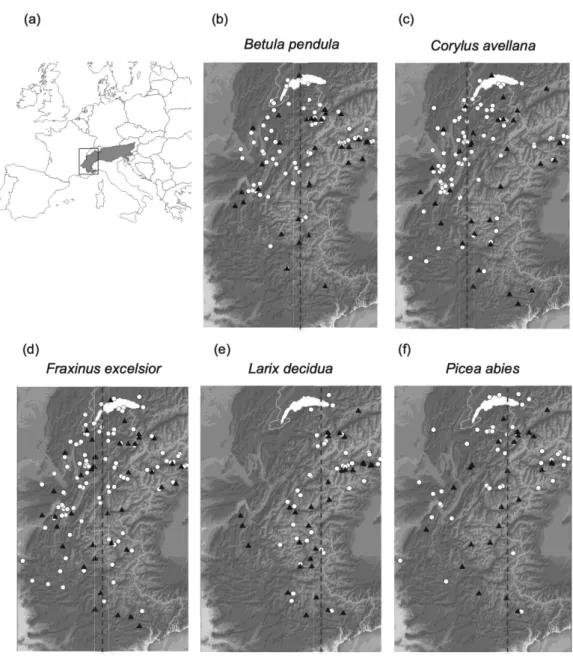
Fig. 1: Locations of the data used for the study. Map showing the location of the study area
402
(western part of the Alps) at the scale of Europe (a). Maps showing the location of sites with
403
phenological records for the five species in the Western Alps (b-f): Betula pendula (birch) (b),
404
Corylus avellana (hazel) (c), Fraxinus excelsior (ash) (d), Larix decidua (larch) (e), Picea abies
405
(spruce) (f). Sites without meteorological station are shown with filled white circles and sites with
406
meteorological station are shown with filled black triangles. The dotted lines correspond to the
407
species-specific longitudes separating West and East sites that defined the sub-datasets for each
408
species (see section 2.4).
409 410 411 412
413
Table 1: Summary of the different models that were compared and the different calibrations, 414
validations and projections that were realized. GDD is the abbreviation of growing degree 415
day function and TL of the threshold lower function. Meteo sites correspond to sites equipped 416
with a meteorological station, no meteo sites corresponds to sites not equipped with a 417
meteorological station, east sites correspond to observation sites East of a species-specific 418
longitudinal threshold, west sites correspond to observation sites West of this threshold. 419
3. Results 421
3.1. Selection of the best models 422
Mixed effects models which best explained budburst dates were generally models 423
including GDD5, and chilling as predicting variables (Appendix B). However, budburst dates 424
of Corylus and Fraxinus were best explained by GDD0 together with chilling. Variance 425
partitioning also indicated an important joint contribution of GDD0 or GDD5 and chilling for 426
all species (Appendix B). However, over all 8 years and all locations, chilling did not explain 427
a significant part of the variance in spring phenology once forcing temperatures were taken 428
into account except in Picea (Appendix B). For further analysis we only present the results of 429
the correlative model with GDD0 or GDD5 (depending of the species) and chilling as 430
variables. 431
The response function to temperature in process-based models that best explained the 432
budburst date was the lower threshold function for Fraxinus and Picea and the Wang 433
function for the three other species for the endodormancy phase; and the sigmoid function for 434
all species for the ecodormancy phase (Appendix C). However, because the differences in 435
efficiency and AICc were very small between models using the Wang function and the 436
threshold function, we selected the lower threshold function for all species for the rest of the 437
analyses, for the sake of parsimony. 438
Process-based models performed the best for Picea and Betula (Fig. 2, Appendix D, 439
Appendix F and Appendix G). However, model error increased with the distance to the mean 440
budburst date, irrespective of the model and the species, with a tendency towards 441
exaggerating early and late budburst dates (predicted dates too early or too late, respectively) 442
(Appendix F and Appendix G). We found no trend in model residuals (observed predicted 443
dates) along elevation, except for Larix for which observed budburst dates tended to occur 444
earlier than predicted by the models at low elevation and reversely at high elevation 445
(Appendix H and Appendix I). 446
All performance indices indicated that correlative models predicted the budburst date 447
more accurately than process-based models whatever the calibration dataset for all species 448
(Appendix D). This result was confirmed by bootstrapped values of RMSE that were 449
significantly lower for correlative models than process-based models for all species (Fig. 2). 450
Performance indices were only slightly better for 2-phase models than 1-phase models (Fig. 451
2, Appendix D). However, comparing the performances for an unusually warm year, i.e. with 452
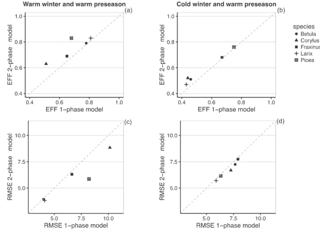
warm winter and warm preseason, we found that 2-phase process-based models performed 453
better for Corylus and Picea (Fig. 3). For the other species, model performance was similar 454
between the one- and 2-phase process-based models. For a typical year with a cold winter and 455
a warm preseason, performance indices were similar between the two types of process-based 456
model for all species (Fig. 3). 457
458
3.2. Model transferability in space 459
Whatever the validation data subset, process-based models provided more accurate 460
projections of the budburst date than correlative models, except for Picea abies for which 461
performed similarly (Fig. 2, Appendix E). Performances were similar between 2-462
phase models and 1-phase models. Process-based models were thus more robust than 463
correlative models. Indeed, while RMSE increased from predictions to projections in 464
correlative models, they remained similar in process-based models (Fig. 2, Appendix E). 465
Therefore, model performance of process-based models was more stable (3.45 and 0.87 mean 466
difference in RMSE between calibration and validation for the correlative and process-based 467
models respectively). 468
Similarly to the predicted dates, error in projected dates increased with the distance to 469
the mean budburst date, irrespective of the model and the species (Appendix F and Appendix 470
G) with exaggerating early and late dates. 471
Model residuals were linearly related to elevation for Corylus and Fraxinus 472
(correlative models only), and Larix (all models), with dates projected slightly too late at low 473
elevation and too early at high elevation (Appendix H and I). 474
475
3.3. Projections of the budburst date in future climatic conditions 476
Evolution across time 477
We compared the projections of the budburst date of the five species by the best 478
correlative model and the best process-based 1-phase and 2-phase models over the historical 479
period and the 21stcentury in the French Alps using climatic data simulated by the ALADIN-480
Climat RCM. Uncertainties in the climatic data (minimum temperatures, maximum 481
temperatures) were similar along the period and should not therefore add a bias across time in 482
the model projections (Appendix J). 483
Model projections differed substantially according to elevation and time period. At 484
low elevation, up to 2050, correlative models and 1-phase models projected a continuous 485
trend for earlier budburst dates -0.08 to -0.16 days/year and -0.09 to -0.12 days/year 486
respectively; Fig. 4 & 5, Appendix K) while 2-phase models showed a much weaker trend for 487
earlier budburst dates (-0.05 to -0.07 days/year; Fig. 4, Appendix K). Models projection 488
dates (-0.27 to -0.48 days/year; Fig. 4, Appendix K), trend weakened in 1-phase models 490
projection (-0.03 to -0.20 days/year; Fig. 4, Appendix K); and vanished or even reverted in 2-491
phase models projection (-0.01 to +0.16 days/year; Fig. 4, Appendix K). 492
At high elevation, correlative models provided astonishing projections with very low 493
interannual variability of budburst dates, a slight trend towards earlier date from 1950 to 2050 494
(-0.005 to -0.07 days/year; Fig. 4, Appendix K) that steepened after 2050 (-0.13 to -0.28 495
days/year; Fig. 4, Appendix K). Process-based models showed a trend for earlier budburst 496
dates (-32 to -46 days) all along the 1950-2100 period. 1-phase models and 2-phase models 497
both projected a remarkably similar trend towards earlier budburst dates all along the 498
historical period and until 2050 (-0.16 to -0.21 days/year; Fig. 4, Appendix K). However, 499
while after 2050, the trend towards earlier budburst dates remained similar between the two 500
process-based models for Larix (-0.42 days/year) and Picea (-0.32 days/year), it weakened in 501
the 2-phase model for the other species (Fig. 4, Appendix K). 502
For Fraxinus, Betula and Picea, 2-phase models episodically projected budburst 503
failure due to endodormancy release failure because of a lack of chilling. This situation 504
occurred especially at low elevation and with an increasing frequency along the 21th century 505
(Fig. 5). 506
507
Variation across space 508
Correlative models projected earlier budburst dates over the French Alps at an 8-km 509
resolution with a trend more pronounced in the outer and southern Alps than in the central 510
Alps where the elevation is higher on average. The contrast between outer and central Alps 511
was the most pronounced for Betula, Larix and Picea (Fig. 6). Reversely, 1-phase and 2-512
phase models projected a steeper trend towards earlier budburst dates in the central Alps than 513
the outer Alps. However, contrary to 1-phase models, 2-phase models projected later dates in 514
the southern Alps for all species, and also in the north of the outer Alps for Larix and Picea 515
(Fig. 6). The contrasted projections between the outer and central Alps were more 516
pronounced for Larix (Fig. 6). 517
518
3.4. Performance of the forward calibrated model 519
The forward calibrated 2-phase model for Larix performed the worst on average 520
compared to other models in predicting the budburst date whatever the calibration data subset 521
(Fig. 2, Appendix D), but nevertheless provided more accurate predictions of early dates than 522
the 2-phase model calibrated with inverse modelling (Appendix L). The model also provided 523
the most accurate projections for the sites without meteorological stations, but not for the 524
other data subsets (Fig. 2, Appendix E). More interestingly, this model was the only one to 525
provide a lower error on average with the validation data subsets than with the calibration 526
data subsets (-0.39 vs +0.65 for 2-phase model and +0.84 for 1-phase model), and thus 527
showed the reverse behavior we usually observe with models of an increased error in external 528
(validation) conditions. Like other models (either correlative or process-based) for Larix 529
decidua, residuals were linearly related to elevation, with projected dates tending to be 530
overestimated at low elevation and underestimated at high elevation (Appendix M). 531
Over the historical period and the 21st century, budburst dates projected by the 532
forward calibrated 2-phase model were very similar to those projected by the 2-phase model 533
either at low or high elevation (Fig. 7). However, the forward calibrated model showed much 534
more frequent endodormancy release failures than the 2-phase model which projected none 535
projected by the forward calibrated model for Larix over the French Alps for each grid cell 537
for the period 1950-2100 (Fig. 6). 538
Fig. 2: Boxplots of bootstrapped values of RMSE (days). Performance of the best models in 540
predicting (a, c, e, g, i) and projecting the budburst date (b, d, f, h, j). Predictions correspond 541
to the budburst dates predicted by the models for their respective calibration dataset: sites 542
with meteorological stations (clear grey); sites West of the species-specific longitudinal 543
threshold (grey); sites East of the species-specific longitudinal threshold (dark grey). 544
Projections correspond to budburst dates predicted by the three different versions of 545
calibrated models for respectively observation sites without meteorological stations (clear 546
grey); observations sites East of the species-specific longitudinal threshold (grey); 547
observation sites West of the species-specific longitudinal threshold (dark grey). Models on 548
the X axis are the same calibrated models on right and left panels which differ only by the 549
datasets used to evaluate the model performance distinguished by the different shades of 550
grey. Correlative 1 refers to the linear mixed model with GDD only. Correlative 2 refers to 551
the linear model with GDD and chilling as variables. PB 1-phase refers to the process-based 552
1-phase model. PB 2-phase refers to the process-based 2-phase model. Forward calibrated PB 553
refers to the forward calibrated process-based 2-phase model. 554
556 557
Fig. 3: Performance (Efficiency a, b; RMSE c, d) of the process-based models in predicting 558
the budburst date of the calibration data subset 1 (sites with meteorological stations) for a 559
year with a warm winter followed by a warm preseason (a, c) and a year with a cold winter 560
followed by a warm preseason (b, d). Process-based 1-phase models use a sigmoid function 561
of temperature for the ecodormancy phase. Process-based 2-phase models use a lower 562
threshold function of temperature for the endodormancy phase and a sigmoid function of 563
temperature for the ecodormancy phase. EFF, model efficiency; RMSE, roots-mean-squared 564
error (days). Model labels as in Fig. 2. 565
566 567
568 569
Fig. 4: Budburst date projected by the correlative 2 model (with GDD and chilling as variables)
570
(blue), the process-based 1-phase (grey) and the process-based 2-phase model (red) in 571
historical climate and future climate according to scenario RCP8.5, in the Alps at low 572 Picea abies Larix decidua Betula pendula Fraxinus excelsior Corylus avellana 1950 2000 2050 2100 1 50 100 150 200 1 50 100 150 200 1 50 100 150 200 1 50 100 150 200 1 50 100 150 200 Year
Correlative 2 PB 1 phase PB 2 phase
Picea abies Larix decidua Betula pendula Fraxinus excelsior Corylus avellana 1950 2000 2050 2100 1 50 100 150 200 1 50 100 150 200 1 50 100 150 200 1 50 100 150 200 1 50 100 150 200
elevation (a, c, e, g, i) and high elevation (b, d, f, h, j). Elevation limits depend on the species. 573
Low elevation: Corylus= 100 to 1000m asl.; Fraxinus= 100 to 1000 m asl.; Betula= 100 to 574
1000 m asl.; Larix= 400 to 1500 m asl. and Picea= 100 to 1500 m asl.. For high elevation: 575
Corylus= 1001 to 2000m asl.; Fraxinus= 1001 to 2000 m asl.; Betula= 1001 to 2300 m asl.; 576
Larix= 1501 to 2700 m asl. and Picea= 1001 to 2500 m asl.. Bold lines indicate the projected 577
mean date and areas indicate the confidence interval of the model. Model labels as in Fig. 2. 578
580
Fig. 5: Percentage of sites showing dormancy breaking failure under climate scenario 582
RCP8.5 in the Alps along the years (a, c, e, g, i) and along the elevation gradient (b, d, f, h, j). 583
Grey dots indicate values for the process-based 2-phase model and black dots indicate values 584
for the forward calibrated process-based 2-phase model. Note that the 2-phase process-based 585
model did not project dormancy breaking failure for Larix decidua. Model labels as in Fig. 2. 586
Fig. 6: Shift in budburst date projected by the correlative (with GDD and chilling as variables)
589
(a, d, g, j, m), the process-based 1-phase (b, e, h, k, n) and 2-phase (c, f, i, l, o) models in the 590
French Alps (spatial resolution: 8 km) between 1950 and 2100 (scenario RCP8.5). Shift was 591
592
and years over the period 1950 to 2100. 593
595
596 597
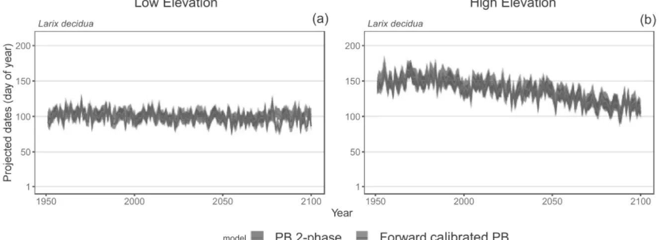
Fig. 7: Budburst date of Larix decidua projected by the 2-phase model (red) and the forward 598
calibrated 2-phase model (yellow) in historical and future climate (scenario RCP8.5) in the 599
Alps at low elevation (400 to 1500 m asl.) (a) and high elevation (1501 to 2700 m asl.) (b). 600
Red curves indicate the mean date projected by the 2-phase model and red areas indicate the 601
confidence interval of the model. Brown curves indicate the mean date projected by the 602
forward calibrated model and orange areas indicate the confidence interval of the model. 603
Because the forward calibrated model showed much more frequent budburst failures due to 604
endodormancy release failures than the 2-phase model, we could not represent the deviation 605
of budburst date projected by the calibrated model over the French Alps for the period 1950-606
2100. Model labels as in Fig. 2. 607 608 609 (b) (a) High Elevation Low Elevation Larix decidua 1950 2000 2050 2100 1 50 100 150 200 Year
model process 2 phase process calibrated
Larix decidua 1950 2000 2050 2100 1 50 100 150 200 ForwardcalibratedPB PB 2-phase
4. Discussion 610
4.1. Process-based phenology models provide more robust projections than correlative 611
models 612
Linear mixed models using chilling days and growing degree days (GDD) were more 613
efficient than process-based models in predicting the budburst date in calibration conditions 614
(i.e. sensu Randin et al., 2006). However, process-based models were more efficient than 615
correlative models to project budburst date in external conditions (except for Picea for which 616
the three model types revealed similar performance). Error in predicted dates and projected 617
dates increased with the distance to the mean budburst date of the calibration datasets, 618
irrespective of the model and the species. This error inflation at the edge of the calibration 619
range leads to exaggerating early and late dates. However, errors were lower for process-620
based models compared to correlative models probably because the former formalize causal 621
relationships between the dependent variable and the independent variables across the range 622
of projection contrary to the latter. Although, these conclusions are dependent on the models 623
we have used for this study the way we chose the models asserts a certain degree of 624
generality to these conclusions because models differed essentially by their structure and not 625
by their predicting variables. 626
Projections of the forward calibrated 2-phase model were not more accurate than 627
those of the other 2-phase models except for sites without meteorological stations. However, 628
it was the only model that did not show an increased error in external conditions. Increased 629
accuracy in this model was mainly achieved through a more accurate prediction of early 630
dates. Our results robustness of process-based models can come additionally from 631
forward parameter estimation, but also that forward parameter estimation is not necessarily 632
the Holy Grail that we should seek. Another study conducted on rice (Nagano et al., 2012; 633
but see Satake et al., 2013) showed that phenology models calibrated by forward estimation 634
actually might perform worse in situ conditions than in controlled conditions and vice versa. 635
This study suggests that either the effect of some abiotic factors and their interactions or the 636
daily variation of these factors in nature might be poorly represented under controlled 637
conditions, and that epigenetic or acclimation effects might interfere. Besides this, results 638
from experiments can sometimes be biased by ontogenetic effects when young cohorts of 639
individuals are used (Vitasse, 2013). Thus, it seems that backward and forward parameter 640
estimations have both biases that come from the same reason, i.e. incomplete sampling of the 641
environmental conditions that affect the phenology, wherever natural or artificial. 642
Therefore, obtaining r 643
a combination of both the experimental approach 644
(forward estimation) and the statistical approach (backward estimation) 645 646 647 648 649 650 651 652 653
Divergence between projections of correlative and 2-phase models in future climatic 654
conditions across the Alps are striking. For all species at high elevation over the 1950-2050 655
period, correlative models projected earlier dates than 2-phase models, while after 2050, 656
projections were similar. Standard deviations of the projected dates before 2050 for 657
correlative models were also surprisingly small, particularly for Larix. This might be due to 658
the fact that the GDD variable was calculated over the same period of the year along the 659
elevation gradient. At high elevation, GDD remains low every year, yielding a low variation 660
in the projected budburst dates, which was particularly marked during the historical period. 661
Because Larix is the species that reaches the tree line, variations of GDD are even lower for 662
this species compared to the four other species. These results highlight the limitations of 663
correlative models to simulate budburst dates when transferred to another spatial or temporal 664
domain. 665
Performance indices were similar between 1-phase models and 2-phase models for 666
predictions and projections in historical conditions, suggesting that so far chilling had no 667
major effect on the budburst date because it was sufficient to fully release endodormancy. 668
Consequently, this means that 1-phase models are complex enough to predict and project 669
budburst dates accurately in historical climatic conditions (Chuine et al., 1999 ; Linkosalo et 670
al., 2008 ; Vitasse et al., 2011). However, 2-phase models provided more accurate 671
predictions of the budburst date for particular recent years with warm winter. This was 672
especially marked for Corylus and Picea. Thus, a certain level of winter warming might have 673
been reached in the Alps, sometimes leading to non-optimal chilling conditions and later 674
dormancy release date compared to colder years. In such situation, the integration of an 675
endodormancy phase in the phenology model clearly increases the projections accuracy. The 676
negative effect of winter warming on endodormancy release in tree species has been shown in 677
a previous study (Asse et al. 2018) and has also been proposed as an explanation of the 678
dampening of the response of budburst to warming temperature over the past 25 years in 679
Europe (Fu et al., 2015). Although 680 681 682 683 684 685
Although chilling was taken into account in the correlative models, they did not 686
project a negative effect of a lack of chilling on the budburst date like the 2-phase process-687
based model. Although the two types of models were calibrated with the same dataset which 688
contained only one exceptionally warm winter (2006-2007) which had a delaying effect on 689
the budburst date (Asse et al., 2018), it seems that only the process-based model was able to 690
capture this important information. 691
692
4.3. Evolution of the budburst date in the Alps over the 21stcentury 693
At low elevation, projected budburst dates were similar until ca. 2050 for all models 694
and for all species, with a weak linear trend towards earlier dates (Fig 5 & 6). This linear 695
trend is due to the warming of spring which accelerates cell elongation while the warming of 696
winter does not affect chilling accumulation until 2050 according to climate projections as 697
previously highlighted by Vitasse et al., (2011) ; Chuine et al., (2016) and Fig. 1 in Guo et 698
al., (2015). However, after 2050, while the linear trend towards earlier dates continues and 699
accelerates in correlative and 1-phase models (although less in the latter and especially for 700
Larix), this trend progressively vanished in 2-phase models. 701
At high elevation, projected budburst dates were similar for all species over the 21st 702
century between 1-phase and 2-phase models, suggesting that at high elevation, chilling 703
requirements could be fulfilled until the end of the 21stcentury. 704
Thus, our results suggest that warmer winters might have opposite effects on spring 705
phenology at high compared to low elevation, by advancing vs delaying dormancy release 706
respectively, and consequently reducing the phenological cline across the elevation gradient.
707
As a consequence, trees might become at increasing risk of late spring frost damage at high
708
elevation compared to low elevation in the upcoming decades. A preview of such situations
709
have already been reported in the Swiss Alps over the last decades (Vitasse et al., 2017,
710
2018). Considering that phenological traits have been shown to be primary determinants of
711
species range (Chuine & Beaubien, 2001; Chuine et al., 2013), a reduced phenological shift
712
across the elevation gradient might in the medium term alter the altitudinal zonation of the
713
vegetation.
714
Our results also support the hypothesis of Vitasse et al., (2017) that winter 715
temperatures are currently actually colder than the optimal chilling temperature at high 716
elevation so that a warming of winter actually increases the number of chilling days and 717
advance endodormancy release, and consequently budburst. Bud endodormancy indeed 718
requires from a few weeks to several months of cold temperature, that can vary from 0°C to 719
12°C depending on the species, to be fully released (Lang et al., 1987; Caffarra et al., 2011a; 720
Malagi et al., 2015). 721
From 1950 to 2100, 2-phase models projected a trend for earlier budburst date in the 722
inner Alps (higher elevations), while they projected either very weak trend toward earlier 723
dates or a trend toward later dates in the outer Alps (lower elevations) (particularly for Larix 724
and Picea), and a trend toward later dates whatever the species in the Southern Alps, which 725
match or approach their southern range limit. In the short term, delaying effect of winter 726
warming on budburst date might be beneficial to trees by reducing the risk of exposure to late 727
spring frost. But in the longer term, it is expected to 728
and at species southern range limit 729
730 731 732 733
photoperiod compensating for a lack of chilling. Integration of this compensatory effect in the 734
models might change substantially the projections of budburst dates for the end of the 21st 735
century for photosensitive species which might be the case for Picea abies (Blümel & 736
Chmielewski, 2012; Gauzere et al., 2017). 737
738
Conclusion 739
Our results showed that (1) process-based phenology models are more robust than 740
correlative model even when they rely entirely on backward estimation (inverse modelling) 741
of their parameter values. (2) They also demonstrated that the robustness of process-based 742
models could be increased, though not substantially, when their calibration could rely on 743
forward estimation. Therefore, the robustness of process-based models seems to come 744
primarily from the explicit description of causal relationships rather than from forward 745
estimation of model parameters, and we advise using, whenever possible, both backward and 746
forward estimation of model parameters. (3) In opposite to correlative models, process-based 747
models projected a reduction in the phenological cline along the elevation gradient for all 748
species by the end of the 21stcentury. This later result suggests that using linear relationships 749
to provide projections for the second part of the 21st century will be vain, especially at low 750
elevation and at species southern range limits. 751
752 753
We are grateful to all the volunteers and staffs of protected areas involved in the 754
Phenoclim program for their help and support for collecting data on the study sites. We also 755
756
Chamonix-Mont-Blanc) for having prepared the temperature data used in this study. We 757
thank the Conservatoire Botanique National Alpin for providing the species occurrence data, 758
and two anonymous referees for their constructive comments on earlier versions of the 759
manuscript. This research project was funded by the Association Nationale de la Recherche et 760
de la Technologie (ANRT). 761
Rhône-Alpes and PACA Regions, French ministry of Transition écologique et solidaire. We 762
thank the Société Académique Vaudoise (SAV) for having kindly provided matching funds. 763
764 765
References 766
Anderson, J.J., Gurarie, E., Bracis, C., Burke, B.J., Laidre, K.L., 2013. Modeling climate 767
change impacts on phenology and population dynamics of migratory marine species. 768
Ecol. Modell. 264, 83 97. doi:10.1016/j.ecolmodel.2013.03.009 769
Asse, D., Chuine, I., Vitasse, Y., Yoccoz, N.G., Delpierre, N., Badeau, V., Delestrade, A., 770
Randin, C.F., 2018. Warmer winters reduce the advance of tree spring phenology 771
induced by warmer springs in the Alps. Agric. For. Meteorol. 252, 220 230. 772
doi:10.1016/j.agrformet.2018.01.030 773
Basler, D., 2016. Evaluating phenological models for the prediction of leaf-out dates in six 774
temperate tree species across central Europe. Agric. For. Meteorol. 217, 10 21. 775
doi:10.1016/j.agrformet.2015.11.007 776
Basler, D., Körner, C., 2012. Photoperiod sensitivity of bud burst in 14 temperate forest tree 777
species. Agric. For. Meteorol. 165, 73 81. doi:10.1016/j.agrformet.2012.06.001 778
Bellon-Maurel, V., Fernandez-Ahumada, E., Palagos, B., Roger, J.M., McBratney, A., 2010. 779
Critical review of chemometric indicators commonly used for assessing the quality of 780
the prediction of soil attributes by NIR spectroscopy. TrAC - Trends Anal. Chem. 781
doi:10.1016/j.trac.2010.05.006 782
Benmoussa, H., Ben Mimoun, M., Ghrab, M., Luedeling, E., 2018. Climate change threatens 783
central Tunisian nut orchards. Int. J. Biometeorol. 62, 2245 2255. doi:10.1007/s00484-784
018-1628-x 785
Blümel, K., Chmielewski, F.M., 2012. Shortcomings of classical phenological forcing models 786
and a way to overcome them. Agric. For. Meteorol. 164, 10 19. 787
doi:10.1016/j.agrformet.2012.05.001 788
Bonhomme, M., Rageau, R., Lacointe, A., Gendraud, M., 2005. Influences of cold 789
deprivation during dormancy on carbohydrate contents of vegetative and floral 790
primordia and nearby structures of peach buds (Prunus persica L. Batch). Sci. Hortic. 791
(Amsterdam). 105, 223 240. doi:10.1016/j.scienta.2005.01.015 792
543. 793
Burghardt, L.T., Metcalf, C.J.E., Wilczek, A.M., Schmitt, J., Donohue, K., 2015. Modeling 794
the Influence of Genetic and Environmental Variation on the Expression of Plant Life 795
Cycles across Landscapes. Am. Nat. 185, 212 227. doi:10.1086/679439 796
Burnham, K.P., Anderson, D.R., 2002. Model selection and multimodel inference: a practical 797
information-theoretic approach, Ecological Modelling. 798
doi:10.1016/j.ecolmodel.2003.11.004 799
Caffarra, A., Donnelly, A., Chuine, I., 2011a. Modelling the timing of Betula pubescens 800
budburst. II. Integrating complex effects of photoperiod into process-based models. 801
Clim. Res. 46, 159 170. doi:10.3354/cr00983 802
Caffarra, A., Donnelly, A., Chuine, I., Jones, M.B., 2011b. Modelling the timing of Betula 803
pubescens budburst. I. Temperature and photoperiod: A conceptual model. Clim. Res. 804
46, 147 157. doi:10.3354/cr00980 805
Cheaib, A., Badeau, V., Boe, J., Chuine, I., Delire, C., Dufrêne, E., François, C., Gritti, E.S., 806
Legay, M., Pagé, C., Thuiller, W., Viovy, N., Leadley, P., 2012. Climate change impacts 807
on tree ranges: Model intercomparison facilitates understanding and quantification of 808
uncertainty. Ecol. Lett. 15, 533 544. doi:10.1111/j.1461-0248.2012.01764.x 809
Chuine, I., 2010. Why does phenology drive species distribution? Philos. Trans. R. Soc. B 810
Biol. Sci. 365, 3149 3160. doi:10.1098/rstb.2010.0142 811
Chuine, I., 2000. A Unified Model for Budburst of Trees. J. Theor. Biol. 207, 337 347. 812