HAL Id: hal-01835132
https://hal.inria.fr/hal-01835132
Submitted on 11 Jul 2018
HAL is a multi-disciplinary open access
archive for the deposit and dissemination of
sci-entific research documents, whether they are
pub-lished or not. The documents may come from
teaching and research institutions in France or
abroad, or from public or private research centers.
L’archive ouverte pluridisciplinaire HAL, est
destinée au dépôt et à la diffusion de documents
scientifiques de niveau recherche, publiés ou non,
émanant des établissements d’enseignement et de
recherche français ou étrangers, des laboratoires
publics ou privés.
Online Feedforward/Feedback Structure Adaptation for
Heterogeneous CACC Strings
Carlos Flores, Vicente Milanés, Fawzi Nashashibi
To cite this version:
Carlos Flores, Vicente Milanés, Fawzi Nashashibi. Online Feedforward/Feedback Structure
Adapta-tion for Heterogeneous CACC Strings. American Control Conference (ACC) 2018, Jun 2018,
Milwau-kee, United States. �hal-01835132�
Online Feedforward/Feedback Structure Adaptation for Heterogeneous
CACC Strings
Carlos Flores, Vicente Milanés and Fawzi Nashashibi.
Abstract— Cooperative Adaptive Cruise Control has been extensively studied in recent years, however most of efforts have been oriented to homogeneous strings control. When a heterogeneous string is formed, the differences between vehicles dynamics introduce disturbances in the closed loop system affecting the string stability. This paper presents an online CACC feedforward adaptation with a fractional-order feedback controller for stable heterogeneous strings of vehicles. A particle filter algorithm is employed to perform an online parameter identification over the preceding vehicle longitudinal model, allowing further adaptation of the control structure. Simulations demonstrate the advantages over conventional homogeneous structures as well as system’s capability to both enhance stability and guarantee string stability regardless the vehicles distribution.
I. INTRODUCTION
In the last years, Cooperative Adaptive Cruise Control (CACC) has become a promising solution for improving traf-fic flow [1] with the introduction of longitudinal automation, ranging sensors and vehicle-to-vehicle (V2V) communica-tion links. Several projects have been deployed to inves-tigate the benefits of CACC and platooning when applied
over conventional vehicles [2], [3], heavy duty trucks1 and
mixed traffic2. These works have proved the advantages
of such techniques on highway driving without requiring major modification of the infrastructure, showing significant improvements in terms of traffic capacity [4].
From a control point of view, CACC approaches require each vehicle to track efficiently, smoothly and with robust-ness its preceding one at a reference distance defined by a spacing policy. Among the different spacing policies, con-stant time gap (CTG) [5] strategy is the most employed since it provides the most intuitive way to set the distance between vehicles as it varies proportionally to the ego-speed. The system gap-regulation performance and its stability strongly depend on the desired time gap–i.e. keeping a car-following formation with shorter time gaps requires more performing reference tracking capabilities–.
String stability plays a key role when it comes to design CACC systems. This concept was firstly introduced by [6] and widely studied in the work of [7], [8] among others. It Carlos Flores and Fawzi Nashashibi are with the Robotics and Intelligent Transportation Systems (RITS) Team, INRIA Paris, 2 Rue Simone Iff, 75012 France {carlos.flores-pino,
fawzi.nashashibi}@inria.fr; Vicente Milanés is with
the Research Department, Renault SAS, 1 Avenue de Golf, 78280 Guyancourt, France{[email protected]}.
1https://www.eutruckplatooning.com/default.aspx 2http://www.gcdc.net/en/
refers to the string capability to attenuate disturbance prop-agations in upstream direction. This can be mathematically interpreted as:
Γ(s) = Zi(s)
Zi−1(s)
; i ≥ 2 (1)
where the term Zi(s) might refer to different vehicle states. A
sufficient condition to guarantee the system string stability is to ensure that the infinite norm of the string stability function
is less or equal than unity for all vehicles–i.e. kΓ(s)k∞ ≤
1; ∀ i ≥ 2. In the case where all the string members have identical dynamics (homogeneous strings), the string stability
can be studied defining Zi(s) as the vehicle position, speed,
acceleration, spacing error or control effort.
However, when the CACC is integrated by vehicles with different dynamics (heterogeneous strings), spacing errors and control effort signals evolve differently for each vehicle, because they are closely dependent to the ego and preceding vehicles’ dynamics. For this reason, this work employs the string stability criterion defined in GCDC 2011 [9].
Regarding to heterogeneous strings, firsts analysis have been presented on [10]. Some first approaches include a graph-based control for multi-lane convoy in [11]. In [12], the effect of different time lags and system delays in an ACC string is studied. A CACC control strategy is proposed in [13], [14] that relies on leader-predecessor topology, showing improvement in the performance and ensuring a bounded spacing error regardless the string configuration–i.e. fast-slow, slow-fast, among others–. Although good results have been obtained, communication with the leader vehicle may not always be available due to congestion or if the string length exceeds the secure communication range. A feedforward/feedback (FF/FB) control strategy (which has been widely employed in the CACC literature [15], [16]) is proposed to control a heterogeneous string in [17], where the effect of having vehicles with different behavior is analysed. The ideal FF/FB controllers in function of the formation dynamics, actuators lag, and communications delays is also revised. The influence of the difference between string ve-hicles’ dynamics is analized in [17], considering an offline set FF controller that filters the preceding vehicle reference signal. However, CACC formations should handle real traffic split/merge maneuvers, which means that the system may face a change of the preceding vehicle, requiring to adapt its structure in real time.
Having this in mind, the objectives of this paper are:
• Mitigating the disturbances introduced by the difference
between vehicles’ dynamics in the string 2018 Annual American Control Conference (ACC)
• Developing a string stable control system for heteroge-neous strings
• Taking into account communication links only available
between the ego and preceding vehicle
• Adapting the control response online in function of
the preceding vehicle dynamics with robustness against modelling uncertainties
This work proposes a FF/FB control strategy which adapts the FF filter in function of the ego and preceding vehicles’ dynamics, guaranteeing string stability. The online adaptation is done applying an identification algorithm based on a Par-ticle Filter (PF) over the received V2V data to determine the preceding vehicle longitudinal behavior. A fractional-order feedback controller is designed to be robust against system disturbances and to guarantee the desired tracking stability within a given loop bandwidth without requiring high control efforts. Simulation results demonstrate the advantages of applying the proposed online-adapted structure over static structures.
II. EMPLOYEDFF/FB STRUCTURE
The following configurations of CACC controllers can be found in the state-of-the-art: leader-predecessor following [13], [14], two-vehicle look-ahead [18], bidirectional control [19] and one-vehicle look-ahead topology [16]. This work considers only preceding vehicle information.
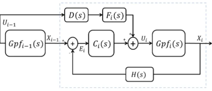
Fig. 1 shows the proposed structure, where
Gpfi(s), Ci(s), H(s), Fi(s) represent the vehicle model
(Xi(s)/Ui(s)), controller, spacing policy and FF filter
respectively. The communication temporal delay is
represented by D(s) = e−θs; θ > 0. The closed-loop
transfer function of the structure in Fig. 1 is given by the expression: Xi(s) Xi−1(s) = D(s)Fi(s) Gpi(s) Gpi−1(s)+ Gpfi(s)Ci(s) 1 + Gpfi(s)Ci(s)Hi(s) ; i ≥ 2 (2) which ∞-norm has to be maintained below unity to ensure
the string stability. The expression Gpi(s) refers to the low
level longitudinal speed behavior (Vreal(s)/Ui(s)) and can
be also defined as Gpi(s) = s · Gpfi(s). Let define Pi(s)
as the term Gpi(s)
Gpi−1(s). For homogeneous strings this term
has no effect since Pi(s) = 1, but when Gpi 6= Gpi−1(s)
the FF loop is affected, compromising the system stability. For this reason, an inverse model control is proposed to be
employed so the effect of Pi(s) in the closed loop is reduced.
This type of control structures has been extensively studied and employed in the literature [20]. The FF controller is set to be of the form Fi(s) = ( ˜Pi(s)Hi(s))−1 where ˜Pi(s)
is an estimation of Pi(s). The term H(s) is employed to
guarantee string stability for every time gap h > 0, in case the FF link presents no communication delays [10], limiting its bandwidth to the interest frequency region as well.
Ideally, perfect tracking of the given reference is achieved
when Fi(s) ≡ (Pi(s)Hi(s))−1. In practice, it is difficult to
determine exactly the term Pi(s) and attain a perfect model
Fig. 1. FF/FB structure employed for CACC systems
inversion. However, a sufficient condition to demonstrate that inverse-model FF/FB structures outperforms FB-only
despite the uncertainty over Pi(s), is to demonstrate that
k ˜Ef f,i(jω)k2 ≤ k ˜Ef b,i(jω)k2 [21], [22]. Assuming no
communication delays, the FF/FB ˜Ef f,i(jω) and FB errors
˜
Ef f,i(jω) functions are given by the expressions:
˜ E(f b,i)(jω) = Xi−1(jω) (1 + Gpfi(jω)Ci(jω)H(jω)) ; ˜ E(f f,i)(jω) = ( ˜Pi(jω) − Pi(jω)) · Xi−1(jω) (1 + Gpfi(jω)Ci(jω)H(jω)) ˜Pi(jω) ; (3)
where it can be observed that the condition is fulfilled if:
| ˜Pi(jω) − Pi(jω)| ≤ | ˜Pi(jω)|; (4)
To satisfy this condition, the objective is to reduce as much
as possible the model uncertainty |∆Pi(jω)| = | ˜Pi(jω) −
Pi(jω)| in the interest frequency region–i.e. the closed loop
bandwidth ω ∈ (0, 1/h]–to yield the best reference tracking as possible, being h the employed time gap. For the
estima-tion of ˜Pi(s) through the FF controller Fi(s), the ego-vehicle
model is assumed to be known; whereas the preceding car model is not due to changes when preceding vehicle leaves
or a cut-in occurs. To approximate ˜Gi−1(s) → Gi−1(s),
the V2V data is employed to estimate Gi−1(s) by using a
parameter identification method.
III. ONLINEPRECEDINGVEHICLEIDENTIFICATION
As explained above, an identification algorithm is applied over the V2V data to adapt online the FF filter in function of the ego and preceding vehicle dynamics. Generally, vehicles’ longitudinal command is based on a hierarchical control strategy composed by a high-level structure that generates a reference speed and a low-level cruise controller in charge of commanding the actuators to track the desired speed. The longitudinal low-level control can be described by a second order model of the form:
Gp(s) =Vreal(s) U (s) = ω2n· e−θs s2+ 2ξω ns + ωn2 (5)
where θ, ωnand ξ represent the transport delay, plant natural
frequency and damping factor. Given that the identification algorithm requires to compute the distance between the model estimations and the observations at each sample time, 50
a discrete version of the model in Eq. 5 is used for the estimation. For this purpose, the Tustin discretization method is applied:
s = 2
T s
1 − z−1
1 + z−1; z ≥ 0 (6)
where T s is the sample time of the identification algorithm and z the discrete operator. Model parameters are determined in real time employing a Particle Filter (PF) algorithm. It provides a fast and robust estimation of the parameters, even if the measurements are corrupted with sensor noise or if the system varies through the time.
A. Online Parameters Modelling Algorithm
An applied version of the
Sequential-Importance-Resampling (SIR) PF proposed in [23] is employed in this work. Since the experimental platform models present a negligible transport delay (θ ≈ 0), only the natural frequency
ωn and damping factor ξ parameters are considered to
describe all the possible longitudinal low level controllers.
Model parameters are assumed to exist as ξ ∈ [ξmin, ξmax]
and ωn ∈ [ωnmin, ωnmax]. This assumption is carried out
because PF algorithms require distribution in bounded pa-rameters spaces. Each particle is defined as a two component
vector: θj = hlog(ωjn), ξji; j ∈ [1, Np], having Np as the
number of particles. The first component is set as the natural frequency logarithm to ensure a more uniform distribution and resampling over the Bode frequency axis.
Initially, a set of particles Θk0 is generated with a random
distribution over the 2D parameter space. Afterwards, the PF is executed online with a sample period T s recommended
to be less than π/ωmax to agree with Nyquist sampling
principle, but high enough to allow the algorithm online execution without data loss. At each time step k, an
input-observation pair huk, yki (reference and measured vehicle
longitudinal speed respectively) is received through V2V
and queued to the 2D vector ¯Zk0:k. The maximum size of
¯
Zk0:k–i.e. Ns–is selected as the highest amount of huk, yki
pairs that can be employed to determine the particles score, allowing real time execution.
At sample time k, the PF computes every particle
es-timations within the time window between k0 to k as
ˆ
yk0:k, employing a discrete-time state space model obtained
combining Eq. 5 and 6. Each particle score is evaluated as the Root Mean Square Error (RMSE) between each particle estimations ˜ykj
0:k and the observations yk0:k along the time
window.
After computing and normalizing each particle score, a resampling process [24] based on such scores is carried out to discard the particles with low fitting and increase the particles population in the areas where high scores have been obtained. For the first executions, as there is no previous knowledge or data to deliver a right parameter estimation with low variance, the preceding vehicle model is
assumed to be similar than the ego-model–i.e. Pi(s) = 1–
. As the vector ¯Zk0:k is filled with input-output data, the
PF algorithm converges to a stable solution presenting low
variance and the estimated parameters ( ˜θk) are updated as
the best scored particle’s parameters (E(θk)). The algorithm
can be summarized as follows:
Algorithm 1 SIR-based PF algorithm for parameters identi-fication
˜
θ1= θego . Assume homogeneous case at beginning
1. Initial sampling at k = 1 θ1j∼ p(θ
j
1); j ∈ [1, Np] . Generate uniform distribution
for θjkin Θkdo . Iterate over the particles
2. Compute particle estimation ˆ
yjk0:k= ComputeEstimations(ujk0:k, θkj) 3. Particle score calculation
wjk= 1/Pk
n=k0(ˆy
j
n− yn)2 . Estimate score with RMSE
end for
4. Normalise weights and output estimation wjk= wik/ PNp j=1w j k E(θk) = argmaxθj k(w j
k) . Estimation with highest score
if σ˜θk≥ σmax then . Supervise estimation convergence
˜
θk= θego . Unstable solution, set homogeneous case
else ˜
θk= E(θk) . Stable PF output, preceding model is
updated with parameters estimation end if
5. Particles resampling . Generate new set Θk+1
p(θjk+1= θkj) = wjk
θk+1j = θjk+1+ νkj; νkj∼ N (0, devθ˜)
The configuration of the PF parameters (particles number
Np, samples number Ns, Gaussian noise standard deviation
devθ˜ and highest tolerated estimation variance σ
max) are
chosen to increase the convergence speed of ˜θk → θreal
(having θreal as the parameters of Gpi−1) and reduce the
expectation variance σθ˜k as much as possible.
The PF outputs the expectation ˜θk = hlog(˜ωn), ˜ξi at each
sample time and such values are employed to configure ˜
Gpi−1(s) in the FF filter Fi(s). Even though the application
of the PF filter yields a good estimation of ˜Gpi−1(s),
mea-surement noise and uncertainties introduce a variance over
the algorithm output with respect to the real model Gpi−1(s).
As explained in Sec. II, the FF/FB structure demands a
low |∆Gpi−1(s)| to guarantee an enhanced reference
track-ing. Therefore, it is required to determine the PF accuracy on the parameters identification task. For this, an offline convergence study is performed modelling different type of vehicles (fast/slow and underdamped/overdamped) following a speed profile with several speed changes. Observation noise is considered as N (0, 0.15). The implemented PF parameters configuration for the study are set as follows:
TABLE I
PFPARAMETERS SET FOR THE CONVERGENCE STUDY
Ns Np T s ωmin ωmax ξmin ξmax iterations
900 200 0.1 0.9 5 0.2 1 10
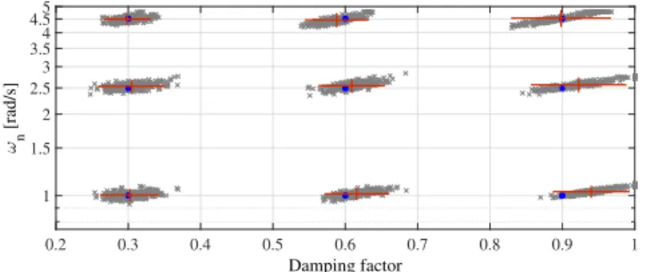
The study is depicted in Fig. 2, where it can be appreciated the parameters estimation of 9 different vehicle dynamics.
0.2 0.3 0.4 0.5 0.6 0.7 0.8 0.9 1 Damping factor 1 1.5 2 2.5 3 3.54 4.55 ωn [rad/s]
Fig. 2. Accuracy study of the PF determining model parameters. In gray the algorithm outputs (250 executions per model), in red the standard deviation illustration for both axis and the ground truth in blue dots
Based on the obtained performance, the preceding vehicle model uncertainty is going to be defined as follows:
ξ = ˜ξ + ∆ξ; |∆ξ| < 0.11;
ωn= ˜ωn· (1 + ∆ωn); |∆ωn| < 0.12;
(7) and consequently, the system performance and stability must
be guaranteed for such uncertainties over the term Gi−1(s).
In this work, the FB controller design is going to be oriented not only to improve the system stability but also to ensure the robustness against perturbations due to the presented uncertainties.
IV. FEEDBACKCONTROLLERDESIGN
Fig. 3 presents the control structure, which FF filter Fi(s)
is adapted with the preceding vehicle model with its uncer-tainties (see Eq. 7). In the literature, FF structures have been widely employed with lead controllers because while FF link improves reference tracking, the lead controller enhances the system damping and FB loop stability [25]. A fractional-order generalization of a lead compensator is employed to gain a more flexible and stable frequency response and avoid high frequency noise amplification. The mathematical form of the fractional-order lead controller is given by:
C(s) = Kp· (1 + sα/ω c) (1 + sα/ω p) ; (8)
where Kp, α, ωc and ωp stand for the controller DC gain,
differentiation order, zero and pole frequencies. The dif-ferentiation order is bounded as α ∈ (0, 2), modifying the magnitude and phase contribution of the controller as +α20 dB/dec and +απ/2 rad/dec respectively. Controller design objectives are:
1) Ensuring kWTiTik∞ ≤ 1; ω > 0 for a time gap of
h = 0.6 to agree with the conclusions obtained in [26]
2) Minimizing kWSiSik∞ to improve the robustness to
perturbations and FB loop stability
3) Reducing the control effort to avoid actuator saturation
kWUiCi(jω)Si(jω)k∞ within the closed loop
band-width
The transfer functions Ti, Si represent the
complemen-tary sensitivity (string stability) and the FB loop
sensi-Fig. 3. Control structure with emphasis in the FF controller and its uncertainty introduced to the FB loop
tivity to perturbations respectively. The template functions WTi, WSi, WUi are selected as follows:
WTi = 1; WSi = s ws+ s/M s ; WUi = 1; (9)
where ws is selected as the plant natural frequency and
Ms= 2. An optimization algorithm (f solve from Matlab) is
applied to determine the controller parameters configuration that minimizes the infinite norms stated in the objectives above. For implementation on discrete embedded systems, a Tustin approximation (Eq. 6) is required with a continued fraction expansion (refer to [27] for more details).
A. Robustness Validation
Three different vehicle dynamics and controllers designed based on their models (Tab. II), are defined for validating the proposed algorithm.
TABLE II
CONTROLLER PARAMETERS CONSIDERING THREE DIFFERENT TYPE OF
DYNAMICS
Vehicle ωn ξ Kp α ωc ωp
Type 1 3.22 0.33 0.98 0.97 8.64 3.89 Type 2 1.85 0.40 0.95 1.06 2.40 5.17 Type 3 1.12 0.67 1.24 1.32 0.29 15.70
Firstly, a sensitivity study is carried out to validate the robustness of the proposed online-adapted FF/FB algorithm. The system performance is evaluated for the worst possible modelling error in Eq. 7 that would result in the highest | ˜Pi(s)|.
The system sensitivity and stability is evaluated in Tab. III
analysing kSi(s)k∞ ≡ kEi(s)/Xi−1(s)k∞. Three control
structures are considered. A FB-only (ACC) where the FF link is replaced with the ego-speed as positive feedback to ensure no stationary state error. A FF/FB approach with the
FF filter set as Fi(s) = 1/H(s) and the FF/FB structure with
the proposed adapted FF filter Fi(s) = ( ˜Pi(s)H(s))−1.
Every possible ego-preceding combination of the three ve-hicle types presented on Tab. II is considered to compare the
performance between FB-only (kSif bk∞), the conventional
FF/FB (kSif f,convk∞) and the proposed FF/FB approach
(kSf f,adapi k∞). The analysis considers no temporal delay on
the communication link and a time gap set of 0.6s. TABLE III
CONTROLLER PARAMETERS FOR THREE DIFFERENT TYPE OF VEHICLES
Ego Prec. kSif bk∞ kSf f,convi k∞ kSf f,adapi k∞
1 1 3.85 0.60 0.60 - 2 3.85 1.20 0.39 - 3 3.85 1.50 0.34 2 1 4.08 4.44 0.60 - 2 4.08 0.49 0.49 - 3 4.08 1.05 0.32 3 1 1.77 21.89 0.72 - 2 1.77 4.76 0.44 - 3 1.77 0.44 0.36
For the FB-only approach, one can see that the system stability is independent from the preceding vehicle dynamics as would be expected from an ACC structure. In the case
where F (s) = 1/H(s), it is clear that when Pi(s) ≈ 1
the performance improves. But when the vehicle dynamics differ, the system stability decreases as the magnitude of
Pi(s) becomes higher, introducing undesired behavior on
the closed loop. When the ego-model has faster dynamics the performance results better, while the worst behavior is obtained when its dynamics are slower than the preceding ones.
For the proposed structure, the system robustness/stability is improved for all scenarios. The enhancement with respect to the other solutions becomes more noticeable as the
magni-tude of Pi(s) is higher. Generally, better results are obtained
with the proposed solution if the ego-vehicle presents a faster model than the preceding one.
Finally, the string stability is analysed in Fig. 4 to demon-strate the fulfilment of the condition in Eq. 1. As in the previous study, the performances of FB-only, FF/FB with the conventional FF filter and the proposed approach are compared for all the possible ego-preceding combinations from Tab. II. As the communication delay directly affects the system string stability, a θ = 0.1s is set.
For the FB-only and the FF/FB structures with conven-tional FF filter, the string stability present an overshoot over the unity at higher frequencies if the ego-model has a low
ωn. This is due to the incapacity of slower vehicles to track
correctly high frequency speed changes. If the ego-model
accounts with a bigger ωn, an overshoot is observed at
lower frequencies given that faster vehicles overreact to the preceding speed changes.
When the proposed adapted-FF filter is employed,
al-though in some frequency regions the magnitude of kTi(s)k
may be higher than for the other static structures, its peak value is maintained below unity in all frequencies for all the possible scenarios, satisfying the string stability condition.
V. SIMULATIONRESULTS
Two scenarios are considered to validate the FF/FB struc-ture. The first where all the vehicles have a previously
10−1 100 101 −20 −15 −10 −5 0 5 10 15 20 Magnitude [dB] Frequency [rad/sec]
Ego = Type 1, Prec = Type 1
10−1 100 101 −20 −15 −10 −5 0 5 10 15 20 Magnitude [dB] Frequency [rad/sec]
Ego = Type 1, Prec = Type 2
10−1 100 101 −20 −15 −10 −5 0 5 10 15 20 Magnitude [dB] Frequency [rad/sec]
Ego = Type 1, Prec = Type 3
10−1 100 101 −20 −15 −10 −5 0 5 10 Magnitude [dB] Frequency [rad/sec]
Ego = Type 2, Prec = Type 1
10−1 100 101 −20 −15 −10 −5 0 5 10 Magnitude [dB] Frequency [rad/sec]
Ego = Type 2, Prec = Type 2
10−1 100 101 −20 −15 −10 −5 0 5 10 Magnitude [dB] Frequency [rad/sec]
Ego = Type 2, Prec = Type 3
10−1 100 101 −20 −15 −10 −5 0 5 Magnitude [dB] Frequency [rad/sec]
Ego = Type 3, Prec = Type 1
10−1 100 101 −20 −15 −10 −5 0 5 Magnitude [dB] Frequency [rad/sec]
Ego = Type 3, Prec = Type 2
10−1 100 101 −20 −15 −10 −5 0 5 Magnitude [dB] Frequency [rad/sec]
Ego = Type 3, Prec = Type 3
Fig. 4. String stability comparison between FB-only (green), FF/FB with the conventional FF filter (blue) and the proposed FF/FB with adaptive FF filter (red)
adapted FF filter considering the ego and preceding vehi-cle models, and the second where all of them have the conventional FF filter F (s) = 1/H(s) as suggested in [10]. Communication links are available with a temporal delay of θ = 0.1s. The string is composed by five vehicles with different dynamics distributed along the formation. The vehicle models parameters are chosen randomly among the
range ωn ∈ [0.9, 5]rad/s and ξ ∈ [0.2, 1]. A detailed
description of the string members is presented in Tab. IV. TABLE IV
SIMULATION PARAMETERS OF STRING VEHICLES
P arameter V eh.1 V eh.2 V eh.3 V eh.4 V eh.5
ωn[rad/s] 3.33 1.54 5 2 2.86
ξ 0.60 0.40 0.90 0.40 0.25
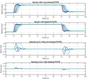
Having the presented string configuration, speed change perturbations are introduced in the leader vehicle. In the upper plots of Fig. 5, the vehicles’ speeds are showed for both scenarios evolving after a leader acceleration and deceleration at t = 55s and t = 80s respectively. The pro-posed system attenuates uniformly the leader speed changes upstream. Whereas for the conventional FF filter, the second and fifth vehicles amplify their precedings’ oscillations. Such behavior is observed when the ego-vehicle has slower dynamics or is less damped than its preceding one, which agrees with the conclusions obtained in [13] and the studies presented in Sec. IV-A.
In the lower plots of Fig. 5 the spacing errors of the controlled vehicles are depicted when using the conventional and the proposed adapted FF filter. The most remarkable differences are that not only the spacing errors are attenuated upstream but also the maximum observed error is reduced from 0.42 to 0.13 meters when applying the online-adapted FF filter.
50 55 60 65 70 75 80 85 90 95 100 Time [s] 9 10 11 Speeds [m/s]
Speeds with conventional FF/FB
50 55 60 65 70 75 80 85 90 95 100 Time [s] 9 10 11 Speeds [m/s]
Speeds with adapted FF/FB
50 55 60 65 70 75 80 85 90 95 100 Time [s] -0.4 -0.2 0 0.2 0.4 Errors [m]
Spacing error with conventional FF/FB
50 55 60 65 70 75 80 85 90 95 100 Time [s] -0.4 -0.2 0 0.2 0.4 Errors [m]
Spacing errors with adapted FF/FB
Fig. 5. Performance comparison between the FF/FB structure with the conventional and the online-adapted FF filter. First to last vehicle (dark to light blue)
A. Simulation with Online Preceding Vehicle Modelling A four vehicle scenario is set with the following string configuration: Type 2, Type 1, Type 3, Type 2; from leader to last vehicle. For the first test, the conventional FF filter is employed for all string members. In the second test, all the vehicles have only previous knowledge of their own models and their preceding vehicles’ models are obtained applying the PF over the received V2V data adapt online FF filter. The same communication delay of θ = 0.1s is considered with a reference time gap of 0.6s between vehicles.
Fig. 6 shows the vehicles’ speed evolution. When the conventional FF filter is applied, the vehicles’ speeds do not evolve uniformly as desired. It can be appreciated that slower vehicles present a higher speed overshoot than the faster ones, which introduces considerable spacing errors (see Fig. 7) that can reach up to 1.6 meters for the case of the third vehicle. When the proposed adapted FF filter is applied, in the first speed step the vehicles’ speeds evolve as in the conventional scenario due to the lack of knowledge of their preceding vehicle model. For the following speed changes, one can observe in Fig. 8 that the modelling parameters converge to their solutions as more V2V data is received to be modelled. This permits a more stable speed evolution as each vehicle is able to adapt the FF filter with the identified preceding vehicle parameters, compensating the dynamics difference. The spacing error peak value is also reduced from 1.8 up to 0.4 meters.
In CACC homogeneous strings, when the leader accel-erates or decelaccel-erates the rest of the string members should face a positive or negative spacing error respectively due to the temporal delay in the V2V link. Instead, when the CACC string is heterogeneous, faster vehicles overreact to
10 15 20 25 30 35 40 Time [sec] 0 1 2 3 4 5 Speeds [m/s]
Speeds with conventional FF/FB
10 15 20 25 30 35 40 Time [sec] 0 1 2 3 4 5 Speeds [m/s]
Speeds with adapted FF/FB
Fig. 6. Vehicles’ speeds along the string from first to last (dark to light blue), with the string members adapting their FF filter online and with the conventional FF filter (top and bottom figures respectively)
10 15 20 25 30 35 40 Time [s] -2 -1 0 1 2 Errors [m]
Spacing errors with conventional FF/FB
10 15 20 25 30 35 40 Time [s] -2 -1 0 1 2 Errors [m]
Spacing errors with adapted FF/FB
Fig. 7. Vehicles’ spacing errors along the string from first to last (black to light blue), with the conventional FF filter and with the string members adapting their FF filter online (top and bottom figures respectively)
the speed change with respect to their slower preceding vehicle, which produces a negative distance error (see 2nd and 4th vehicle in upper plot of Fig. 7). If the ego-vehicle accounts with slower dynamics, the spacing error becomes positive as would be expected towards an increment in the leader speed but higher than desired due to the ego-vehicle limitation to track efficiently its faster preceding vehicle speed changes. This also agrees with the results obtained in Sec. IV-A.
To deal with this problem, the adaptive FF filter is config-ured to process the preceding vehicle’s reference considering both vehicles’ models. This can be appreciated on the lower plot of Fig. 7, where for the first speed change in time t=10s the spacing errors evolve differently; but as each vehicle adapts its structure, not only the errors’ peak values are reduced but also their evolution results more likely as an homogeneous string scenario (positive or negative speed changes produce spacing errors of equal sign).
VI. CONCLUSIONS
An online adapted FF/FB control structure to deal with the CACC heterogeneous string challenge has been proposed, analysed and validated through simulation. Results show that by adapting the FF filter online considering the ego and preceding vehicle models, the disturbances introduced by the 54
10 20 30 40 Time [sec] 1 2 3 4 5 ωn [rad/s], ξ
Leader Modelling (Type 2)
10 20 30 40 Time [sec] 1 2 3 4 5 ωn [rad/s], ξ
First follower Modelling (Type 1)
10 20 30 40 Time [sec] 1 2 3 4 5 ω n [rad/s], ξ
Second follower Modelling (Type 3)
Fig. 8. Model parameters identification by the PF filter of the first, second and third follower vehicles. In red and green the estimation of ωnand ξ
respectively
vehicles dynamics difference can be attenuated and string stability can be ensured for constant time gap CACC. A PF has been proposed to identify the preceding vehicle model parameters online, using the V2V data. Analysis show that although the PF outputs the parameters within a estimation range, the proposed FB fractional-order lead controller is able to provide an enhanced reference tracking task, as well as ensure the string stability even for the worst uncertainty over the preceding vehicle model. Simulation results demon-strate that the proposed online adapted FF/FB structure outperforms structures that does not take into consideration the difference between vehicles’ dynamics, not only in terms of string stability but also on the spacing error regulation task. Future work includes considering uncertainties over the ego-vehicle model, emergency situations and tests over real platforms.
ACKNOWLEDGMENTS
This work has been founded by French Research Agency through the VALET project (ANR-15-CE22-0013). The au-thors would like to thank PhD. Raoul de Charette for valuable discussions during the development of this work.
REFERENCES
[1] S. E. Shladover, C. Nowakowski, X.-Y. Lu, and R. Ferlis, “Cooperative adaptive cruise control: Definitions and operating concepts,” Trans-portation Research Record: Journal of the TransTrans-portation Research Board, no. 2489, pp. 145–152, 2015.
[2] R. Rajamani and S. Shladover, “An experimental comparative study of autonomous and co-operative vehicle-follower control systems,” Transportation Research Part C: Emerging Technologies, vol. 9, no. 1, pp. 15–31, 2001.
[3] J. Ploeg, D. van Sambeek, A. Serrarens, and N. E. Ghouti, “” connect & drive ” c&d c-acc for reducing congestion dynamics,” in 16th ITS World Congress and Exhibition on Intelligent Transport Systems and Services, 2009.
[4] B. Van Arem, C. J. Van Driel, and R. Visser, “The impact of cooperative adaptive cruise control on traffic-flow characteristics,” IEEE Transactions on Intelligent Transportation Systems, vol. 7, no. 4, pp. 429–436, 2006.
[5] D. Swaroop and K. Rajagopal, “A review of constant time headway policy for automatic vehicle following,” in Intelligent Transportation Systems, 2001. Proceedings. 2001 IEEE. IEEE, 2001, pp. 65–69. [6] D. Swaroop and J. K. Hedrick, “String stability of interconnected
systems,” IEEE transactions on automatic control, vol. 41, no. 3, pp. 349–357, 1996.
[7] J. Ploeg, D. P. Shukla, N. van de Wouw, and H. Nijmeijer, “Controller synthesis for string stability of vehicle platoons,” IEEE Transactions on Intelligent Transportation Systems (ITS), vol. 15, no. 2, pp. 854– 865, Apr. 2014.
[8] R. Vugts, “String-stable cacc design and experimental validation,” Diss. Technische Universiteit Eindhoven, 2010.
[9] J. Ploeg, S. Shladover, H. Nijmeijer, and N. van de Wouw, “Intro-duction to the special issue on the 2011 grand cooperative driving challenge,” IEEE Transactions on Intelligent Transportation Systems, vol. 13, no. 3, pp. 989–993, 2012.
[10] G. J. Naus, R. P. Vugts, J. Ploeg, M. J. van de Molengraft, and M. Steinbuch, “String-stable cacc design and experimental validation: A frequency-domain approach,” IEEE Transactions on vehicular tech-nology, vol. 59, no. 9, pp. 4268–4279, 2010.
[11] I. Navarro, F. Zimmermann, M. Vasic, and A. Martinoli, “Distributed graph-based control of convoys of heterogeneous vehicles using curvi-linear road coordinates,” in Intelligent Transportation Systems (ITSC), 2016 IEEE 19th International Conference on. Ieee, 2016, pp. 879– 886.
[12] L. Xiao and F. Gao, “Practical string stability of platoon of adaptive cruise control vehicles,” IEEE Transactions on intelligent transporta-tion systems, vol. 12, no. 4, pp. 1184–1194, 2011.
[13] E. Shaw and J. K. Hedrick, “String stability analysis for heterogeneous vehicle strings,” in American Control Conference, 2007. ACC’07. IEEE, 2007, pp. 3118–3125.
[14] ——, “Controller design for string stable heterogeneous vehicle strings,” in Decision and Control, 2007 46th IEEE Conference on. IEEE, 2007, pp. 2868–2875.
[15] V. Milanés, S. E. Shladover, J. Spring, C. Nowakowski, H. Kawazoe, and M. Nakamura, “Cooperative adaptive cruise control in real traffic situations,” IEEE Transactions on Intelligent Transportation Systems, vol. 15, no. 1, pp. 296–305, 2014.
[16] J. Ploeg, B. T. Scheepers, E. Van Nunen, N. Van de Wouw, and H. Nijmeijer, “Design and experimental evaluation of cooperative adaptive cruise control,” in Intelligent Transportation Systems (ITSC), 2011 14th International IEEE Conference on. IEEE, 2011, pp. 260– 265.
[17] C. Wang and H. Nijmeijer, “String stable heterogeneous vehicle platoon using cooperative adaptive cruise control,” in Intelligent Trans-portation Systems (ITSC), 2015 IEEE 18th International Conference on. IEEE, 2015, pp. 1977–1982.
[18] J. Ploeg, D. P. Shukla, N. van de Wouw, and H. Nijmeijer, “Controller synthesis for string stability of vehicle platoons,” IEEE Transactions on Intelligent Transportation Systems, vol. 15, no. 2, pp. 854–865, 2014.
[19] J. C. Zegers, E. Semsar-Kazerooni, J. Ploeg, N. van de Wouw, and H. Nijmeijer, “Consensus-based bi-directional cacc for vehicular platooning,” in American Control Conference (ACC), 2016. IEEE, 2016, pp. 2578–2584.
[20] Y. Xie and A. Alleyne, “Robust two degree-of-freedom control for mimo system with both model and signal uncertainties,” IFAC Pro-ceedings Volumes, vol. 47, no. 3, pp. 9313–9320, 2014.
[21] S. Devasia, “Should model-based inverse inputs be used as feed-forward under plant uncertainty?” IEEE Transactions on Automatic Control, vol. 47, no. 11, pp. 1865–1871, 2002.
[22] A. Faanes and S. Skogestad, “Feedforward control under the presence of uncertainty,” in European Control Conference (ECC), 2003. IEEE, 2003, pp. 1387–1392.
[23] N. J. Gordon, D. J. Salmond, and A. F. Smith, “Novel approach to nonlinear/non-gaussian bayesian state estimation,” in IEE Proceedings F (Radar and Signal Processing), vol. 140, no. 2. IET, 1993, pp. 107–113.
[24] C. M. Carvalho, M. S. Johannes, H. F. Lopes, N. G. Polson et al., “Particle learning and smoothing,” Statistical Science, vol. 25, no. 1, pp. 88–106, 2010.
[25] C. Flores, V. Milanés, and F. Nashashibi, “Using fractional calculus for cooperative car-following control,” in IEEE 19th International Con-ference on Intelligent Transportation Systems (ITSC), 2016. IEEE, 2016, pp. 907–912.
[26] C. Nowakowski, J. O’Connell, S. E. Shladover, and D. Cody, “Co-operative adaptive cruise control: Driver acceptance of following gap settings less than one second,” in Proceedings of the Human Factors and Ergonomics Society Annual Meeting, vol. 54, no. 24. SAGE Publications Sage CA: Los Angeles, CA, 2010, pp. 2033–2037. [27] I. Podlubny et al., “Using continued fraction expansion to discretize
fractional order derivatives,” Nonlinear Dyn, vol. 38, no. 1-4, pp. 155– 170, 2004.