HAL Id: hal-02308126
https://hal.inria.fr/hal-02308126v2
Preprint submitted on 2 Apr 2021HAL is a multi-disciplinary open access archive for the deposit and dissemination of sci-entific research documents, whether they are pub-lished or not. The documents may come from teaching and research institutions in France or abroad, or from public or private research centers.
L’archive ouverte pluridisciplinaire HAL, est destinée au dépôt et à la diffusion de documents scientifiques de niveau recherche, publiés ou non, émanant des établissements d’enseignement et de recherche français ou étrangers, des laboratoires publics ou privés.
Distributed under a Creative Commons Attribution - NonCommercial - NoDerivatives| 4.0 International License
Alexandre Routier, Ninon Burgos, Mauricio Díaz, Michael Bacci, Simona
Bottani, Omar El-Rifai, Sabrina Fontanella, Pietro Gori, Jérémy Guillon,
Alexis Guyot, et al.
To cite this version:
Alexandre Routier, Ninon Burgos, Mauricio Díaz, Michael Bacci, Simona Bottani, et al.. Clinica: an open source software platform for reproducible clinical neuroscience studies. 2021. �hal-02308126v2�
Clinica: an open-source software platform for reproducible
1
clinical neuroscience studies
2
Alexandre Routier1,2,3,4,5,6, Ninon Burgos2,3,4,5,6,1, Mauricio Díaz6, Michael Bacci1,2,3,4,5,6, Simona
3
Bottani1,2,3,4,5,6 , Omar El-Rifai1,2,3,4,5,6, Sabrina Fontanella2,3,4,5,6,1, Pietro Gori1,2,3,4,5,6, Jérémy
4
Guillon2,3,4,5,6,1, Alexis Guyot2,3,4,5,6,1, Ravi Hassanaly2,3,4,5,6,1, Thomas Jacquemont2,3,4,5,6,1, Pascal
5
Lu2,3,4,5,6,1, Arnaud Marcoux2,3,4,5,6,1, Tristan Moreau2,3,4,5,6,8, Jorge Samper-González2,3,4,5,6,1 ,
6
Marc Teichmann2,3,4,5,6,8,9, Elina Thibeau-Sutre2,3,4,5,6,1, Ghislain Vaillant2,3,4,5,6,1, Junhao
7
Wen2,3,4,5,6,1, Adam Wild2,3,4,5,6,1, Marie-Odile Habert10,11,12, Stanley Durrleman1,2,3,4,5,6, Olivier
8
Colliot2,3,4,5,6,1,*
9
1 Inria, Aramis project-team, Paris, France
10
2 Sorbonne Université, Paris, France
11
3 Institut du Cerveau – Paris Brain Institute - ICM, Paris, France
12
4 Inserm, Paris, France
13
5 CNRS, Paris, France
14
6 AP-HP, Hôpital de la Pitié-Salpêtrière, Paris, France
15
7 Inria Paris, SED, Paris, France
16
8 Institut du Cerveau – Paris Brain Institute - ICM, Paris, France
17
9 Department of Neurology, Institute for Memory and Alzheimer's Disease, Pitié-Salpêtrière Hospital,
18
AP-HP, Paris, France 19
10 Sorbonne Université, CNRS, INSERM, Laboratoire d’Imagerie Biomédicale, LIB, Paris, France
20
11 AP-HP, Hôpital Pitié-Salpêtrière, Médecine Nucléaire, Paris, France
21
12 Centre d’Acquisition et Traitement des Images (CATI), www.cati-neuroimaging.com
22 23
* Correspondence:
24
Olivier Colliot, PhD – [email protected] 25
ICM – Paris Brain Institute 26
ARAMIS team Pitié-Salpêtrière Hospital 27
47-83, boulevard de l’Hôpital, 75651 Paris Cedex 13, France 28
Keywords: Neuroimaging, Software, Pipeline, Data processing, Machine learning, Multimodal
29
data.
2
Abstract
31
We present Clinica (www.clinica.run), an open-source software platform designed to make clinical 32
neuroscience studies easier and more reproducible. Clinica aims for researchers to i) spend less time 33
on data management and processing, ii) perform reproducible evaluations of their methods, and iii) 34
easily share data and results within their institution and with external collaborators. The core of Clinica 35
is a set of automatic pipelines for processing and analysis of multimodal neuroimaging data (currently, 36
T1-weighted MRI, diffusion MRI and PET data), as well as tools for statistics, machine learning and 37
deep learning. It relies on the brain imaging data structure (BIDS) for the organization of raw 38
neuroimaging datasets and on established tools written by the community to build its pipelines. It also 39
provides converters of public neuroimaging datasets to BIDS (currently ADNI, AIBL, OASIS and 40
NIFD). Processed data include image-valued scalar fields (e.g. tissue probability maps), meshes, 41
surface-based scalar fields (e.g. cortical thickness maps) or scalar outputs (e.g. regional averages). 42
These data follow the ClinicA Processed Structure (CAPS) format which shares the same philosophy 43
as BIDS. Consistent organization of raw and processed neuroimaging files facilitates the execution of 44
single pipelines and of sequences of pipelines, as well as the integration of processed data into statistics 45
or machine learning frameworks. The target audience of Clinica is neuroscientists or clinicians 46
conducting clinical neuroscience studies involving multimodal imaging, and researchers developing 47
advanced machine learning algorithms applied to neuroimaging data. 48
3
1 Introduction
49
Neuroimaging plays an important role in clinical neuroscience studies. While the meaning of clinical 50
neuroscience studies may vary, we use it to refer to studies involving human participants (i.e. patients 51
with neurological and psychiatric diseases, and control subjects) explored with multimodal data 52
(neuroimaging, clinical and cognitive evaluations, genetic data...) and most often involving 53
longitudinal follow-up. Carrying out such studies involves many data analysis steps including image 54
pre-processing, extraction of image-derived measurements and statistical analysis, thus requiring a 55
wide range of expertise. A similar situation is faced by researchers in machine learning for 56
neuroimaging: various steps are needed to extract features that are then fed to advanced learning 57
algorithms. 58
The first issue met when working on clinical studies concerns the organization of neuroimaging 59
datasets within or between institutions. The lack of a consistent structure makes arduous the sharing or 60
reuse of data. This is true for in-house, but also for publicly available neuroimaging datasets. Another 61
consequence of the lack of standard is the difficulty to apply automatic pipelines (e.g. extraction of 62
neuroimaging features, statistical analysis or machine learning) and to perform quality assurance. The 63
second issue faced by researchers processing data from clinical studies is related to the high number of 64
software packages, such as FreeSurfer1 (Fischl, 2012), FMRIB Software Library (FSL)2 (Jenkinson et
65
al., 2012) or Statistical Parametric Mapping3 (SPM) (Friston et al., 2007), that exist in the community.
66
Researchers have to understand the methodology behind each tool (e.g. segmentation, registration, etc.) 67
and master them from a programming perspective before being able to combine them and develop 68
image processing pipelines. Moreover, such “handicraft” approach makes it difficult to transmit tools 69
and knowledge, and to merge and share results of several studies due to the heterogeneous organization 70
of outputs. Finally, the difficulty to access or share both raw and processed neuroimaging data hinders 71
the reproducibility of neuroimaging studies (Poline et al., 2012). 72
Major progress has been made in the last years to ease neuroimaging studies. First, difficulties 73
related to the heterogeneity of image processing tools have been partly handled by the Nipype 74
(Neuroimaging in Python – Pipelines and Interfaces) software package4 (Gorgolewski et al., 2011).
75
Nipype is an open-source Python project that provides a uniform environment facilitating interaction 76
between neuroimaging software tools or algorithms, regardless of their programming language, within 77
a single workflow. Later, the issues related to the organization of the clinical and imaging data have 78
been tackled by the Brain Imaging Data Structure (BIDS) (Gorgolewski et al., 2016), a new standard 79
from the community for the community. The BIDS standard is based on a file hierarchy rather than on 80
a database management system, thus facilitating its deployment in any environment. Thanks to its clear 81
and simple way to describe neuroimaging and behavioral data, the BIDS standard has been easily 82
adopted by the neuroimaging community. Organizing a dataset following the BIDS hierarchy 83
simplifies the execution of neuroimaging software tools, resulting in the development of user-friendly 84
software. For instance, BIDS Apps (Gorgolewski et al., 2017) provides a set of pipelines for the 85
processing of neuroimaging data that follow a BIDS hierarchy. Currently, it mainly wraps 86
neuroimaging software packages from the community into a Docker image and is used via a command 87
1http://surfer.nmr.mgh.harvard.edu/ 2https://fsl.fmrib.ox.ac.uk/
3http://www.fil.ion.ucl.ac.uk/spm/ 4https://nipype.readthedocs.io
4
line interface. Moreover, the Nilearn5 (Abraham et al., 2014) package facilitates the application of
88
advanced machine learning approaches to neuroimaging data. To that purpose, it leverages the scikit-89
learn library6 (Pedregosa et al., 2011) and provides tools for handling and visualizing different types
90
of neuroimaging data and building predictive models. 91
Nevertheless, carrying out a multimodal neuroimaging study remains challenging due to the 92
know-how necessary to grasp each modality and tool involved. While technical implementation has 93
been facilitated by Nipype, the development of a pipeline still requires substantial programming skills 94
and time to master both the neuroimaging software tools and Nipype. While the BIDS standard is being 95
adopted by the scientific community, not all public neuroimaging datasets provide a BIDS version of 96
their data. Besides, performing a single or multimodal neuroimaging study will also require 97
methodological expertise. For instance, a classification study of healthy subjects and patients with a 98
neurodegenerative disease using 18F-fluorodeoxyglucose positron emission tomography (FDG PET)
99
could involve notions of multimodal registration between FDG PET and T1-weighted magnetic 100
resonance imaging (MRI), tissue segmentation of T1-weighted (T1w) MRI, PET partial volume 101
correction, normalization into a standard space, and machine learning-based classification, as well as 102
know-how of the tools used to perform these steps. Moreover, the image processing steps need to be 103
chained from one to the other and the absence of data organization for processed neuroimages makes 104
data analysis more complex. Finally, the neuroimaging features generated by the pipelines need to be 105
correctly connected to statistical or machine learning frameworks. 106
Clinica (www.clinica.run) aims to make clinical research studies easier and pursues the 107
community effort of reproducibility. The core of Clinica is a set of automatic pipelines for processing 108
and analysis of multimodal neuroimaging data (currently, T1w MRI, diffusion MRI and PET data), as 109
well as tools for statistics, machine learning and deep learning. Clinica relies on tools written by the 110
scientific community and provides converters of public neuroimaging datasets to BIDS, processing 111
pipelines and organization for processed files, statistical analysis, and machine learning algorithms. 112
The target audience is mainly of two types. First, neuroscientists or clinicians conducting 113
clinical neuroscience studies involving multimodal imaging, typically not experts in image processing 114
for all of the involved imaging modalities or in statistical analysis. They will benefit from a unified set 115
of tools covering the complete set of steps involved in a study (from raw data to statistical analysis). 116
Second, researchers developing advanced machine learning algorithms, typically not experts in brain 117
image analysis. They will benefit from tools to convert public datasets into BIDS, fully automatic 118
feature extraction methods, and baseline classification algorithms to which they could compare their 119
results. Overall, we hope that Clinica will allow users to spend less time on data management and 120
processing, to perform reproducible evaluations of their methods, and to easily share data and results 121
within their institution and with external collaborators. 122
5https://nilearn.github.io 6https://scikit-learn.org/
5
2 Clinica overview
123
Clinica is an open-source software platform for reproducible clinical neuroimaging studies. It can take 124
as inputs different neuroimaging modalities, currently anatomical MRI, diffusion MRI and PET. 125
Clinica provides processing pipelines that involve the combination of different software packages. It 126
currently relies on FreeSurfer (Fischl, 2012), FSL (Jenkinson et al., 2012), SPM (Frackowiak et al., 127
1997), Advanced Normalization Tools (ANTs)7 (Avants et al., 2014a), MRtrix38 (Tournier et al.,
128
2012), and the PET Partial Volume Correction (PETPVC) toolbox9 (Thomas et al., 2016). The
129
pipelines are written using Nipype (Gorgolewski et al., 2011). Features extracted with the different 130
pipelines can be used as inputs to statistical analysis, which relies on SPM (Frackowiak et al., 1997) 131
and SurfStat10 (Worsley et al., 2009), or machine learning analysis, which relies on scikit-learn
132
(Pedregosa et al., 2011) and PyTorch (Paszke et al., 2019). 133
Input neuroimaging data are expected to follow the BIDS data structure (Gorgolewski et al., 134
2016), as explained in section 3.2. Since this new standard has only recently been adopted by the 135
community, not all public neuroimaging datasets are yet proposed in BIDS format. To facilitate the 136
adoption of BIDS, Clinica curates several publicly available neuroimaging datasets and provides tools 137
to convert them into the BIDS format. Processed data are organized following the ClinicA Processed 138
Structure (CAPS) format, detailed in section 3.3, which shares the same philosophy as BIDS. Finally, 139
a set of tools is provided to handle input and output data generated by Clinica, thus facilitating data 140
management or connection to statistical or machine learning analysis. 141
The main functionalities of Clinica are described in the paper, but for further details the reader 142
can refer to the documentation available on the website11. For each pipeline, the reader will find a
143
description of its functionalities, a list of the tools on which it relies, an example showing how to run 144
the pipeline, and a description of the outputs generated. The documentation of a pipeline can have 145
several levels of reading, which are respectively targeting people new or familiar with neuroimaging 146
and scientists working on pattern recognition and machine learning. User support is handled through a 147
forum12 as well as using the issue tracker on GitHub13.
148 149 7https://stnava.github.io/ANTs/ 8http://mrtrix.org 9https://github.com/UCL/PETPVC 10http://www.math.mcgill.ca/keith/surfstat/ 11http://www.clinica.run/doc 12https://groups.google.com/g/clinica-user 13https://github.com/aramis-lab/clinica/issues
6
150
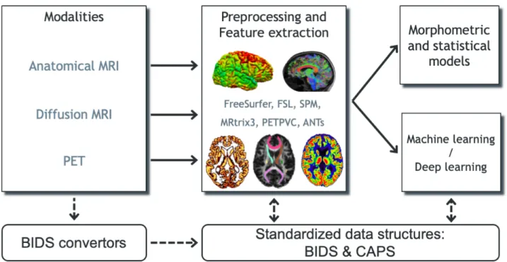
Figure 1. Overview of Clinica’s functionalities. Clinica provides processing pipelines for MRI and
151
PET images that involve the combination of different software packages, and whose outputs can be 152
used for statistical or machine learning analysis. Clinica expects data to follow the Brain Imaging Data 153
Structure (BIDS) and provides tools to convert public neuroimaging datasets into the BIDS format. 154
Output data are stored using the ClinicA Processed Structure (CAPS). 155
156
3 Clinica environment
157
3.1 Software architecture of Clinica
158
The core of Clinica is written in Python and mainly relies on the Nipype framework (Gorgolewski et 159
al., 2011) to create pipelines. Python dependencies also include NumPy (van der Walt et al., 2011), 160
NiBabel (Brett et al., 2019), Pandas (McKinney, 2010), NIPY, SciPy (Jones et al., 2001), scikit-learn 161
(Pedregosa et al., 2011), scikit-image (van der Walt et al., 2011), nilearn (Abraham et al., 2014) and 162
PyTorch (Paszke et al., 2019). 163
Clinica is provided to the end user in the form of a Python package distributed through Python 164
Package Index (PyPI) and can simply be installed by typing pip install clinica through the 165
terminal, within a virtual environment. 166
The main usage of Clinica is through the command line, which is facilitated by the support of 167
autocompletion. The commands are gathered into four main categories. The first category of command 168
line (clinica run) allows the user to run the different pipelines on neuroimaging datasets following 169
a BIDS or CAPS hierarchy. The clinica convert category allows the conversion of publicly 170
available neuroimaging datasets into a BIDS hierarchy. To help with data management, the clinica 171
iotools category comprises a set of tools that allows the user to handle BIDS and CAPS datasets, 172
including generating lists of subjects or merging all tabular data into a single TSV file for analysis with 173
external statistical software packages. Finally, the last category (clinica generate) is dedicated to 174
7
developers and currently generates the skeleton for a new pipeline. Examples of command line can be 175
found in Table 1. 176
177
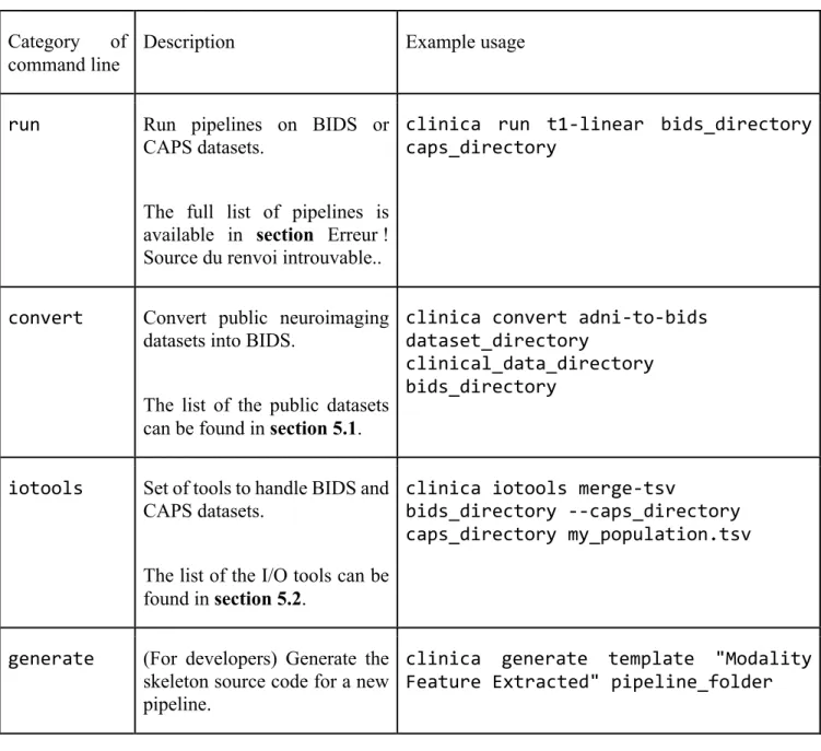
Table 1. Categories of command line
178
Category of command line
Description Example usage
run Run pipelines on BIDS or CAPS datasets.
The full list of pipelines is available in section Erreur ! Source du renvoi introuvable..
clinica run t1-linear bids_directory caps_directory
convert Convert public neuroimaging datasets into BIDS.
The list of the public datasets can be found in section 5.1.
clinica convert adni-to-bids dataset_directory
clinical_data_directory bids_directory
iotools Set of tools to handle BIDS and CAPS datasets.
The list of the I/O tools can be found in section 5.2.
clinica iotools merge-tsv
bids_directory --caps_directory caps_directory my_population.tsv
generate (For developers) Generate the skeleton source code for a new pipeline.
clinica generate template "Modality Feature Extracted" pipeline_folder
3.2 Input data with the BIDS standard
179
When dealing with multiple datasets, it is difficult to automate the execution of neuroimaging pipelines 180
since their organization may vary from each other or even within each individual dataset. If we consider 181
neuroimaging datasets involving many participants, the lack of a clear structure will necessitate a large 182
amount of time to curate these databases and make them easily usable. Besides, large databases are 183
often associated with database management systems, which involve additional technical and financial 184
resources to be maintained. 185
8
BIDS (Gorgolewski et al., 2016) is a community standard enabling the storage of multiple 186
neuroimaging modalities and behavioral data. The BIDS standard provides a unified structure and 187
makes easier the development and distribution of code that uses neuroimaging datasets. Moreover, the 188
BIDS format is based on a file hierarchy rather than on a database management system, thus avoiding 189
the installation and maintenance of additional software. As a result, BIDS can be easily deployed in 190
any environment. The specification is intentionally based on simple file formats and folder structures 191
to reflect current laboratory practices, which makes it accessible to a wide range of scientists coming 192
from different backgrounds. People unfamiliar with the BIDS format can see an example of a BIDS 193
folder in Figure 3. 194
For these reasons, we also adopted this standard and Clinica expects that the input data are 195
BIDS-compliant for the execution of pipelines. Note that if a cross-sectional dataset (i.e. with no 196
session folder) is provided, Clinica will interactively propose to convert the cross-sectional dataset 197
into a longitudinal dataset with a unique session. 198
199
3.3 Input/Output data with the CAPS structure
200
Clinica has its own specifications for storing processed data, called CAPS (ClinicA Processed 201
Structure). Of note, there exists an ongoing initiative called BIDS-derivatives that aims to provide a 202
BIDS standard for processed data. However, we wrote the CAPS specification before the start of the 203
BIDS-derivatives which explains why Clinica does not use the latter. Moreover, in their current state, 204
several outputs needed by Clinica are not covered or well adapted. In particular, the notion of group 205
does not exist yet. Nonetheless, we made humble contributions to BIDS-derivatives and we aim to 206
increasingly contribute. Ultimately, the two specifications will probably converge. 207
Processed data include image-valued scalar fields (e.g. segmentation labels, tissue maps), 208
meshes, mesh-valued scalar fields (e.g. cortical thickness maps), deformation fields, scalar outputs 209
(e.g. volumes, regional averages), etc. Carrying out a neuroimaging study often involves the 210
combination of different pipelines or the chaining of a pipeline to another one. This is the case for 211
multimodal studies where processed outputs from a modality will be inputs for another pipeline, but it 212
is also true for studies involving a single modality: features extracted from one or several pipelines are 213
usually connected to statistical or machine learning frameworks. Finally, a structured organization for 214
processed data will ease the access and sharing of data, thus improving the reproducibility of 215
neuroimaging studies. 216
The CAPS format defines a hierarchy for the Clinica processed data. The idea is to include in 217
a single folder all the results generated by the different pipelines and to organize the data following the 218
main patterns of the BIDS specification. CAPS folders are kept separate from the raw data. Indeed, 219
when processing data, it is very common to have the raw dataset located on a separated storage or read-220
only storage, while ongoing processed data are located on a separate location or on a faster data storage. 221
Another notion we often meet in neuroimaging studies is the notion of group, e.g. template 222
creation from a set of subjects or statistical analysis of a population. To handle these situations, we 223
simply add a level to the CAPS folder hierarchy. While pipeline outputs for individuals are stored in 224
the subjects folder, results of group studies are stored in the groups folder together with the set of 225
participants involved. For instance, an AD group label could be used when a template is created for a 226
group of Alzheimer’s disease patients. Any time this AD template is used, the group_label is 227
provided to identify the pipeline outputs obtained for this group. The group HCvsAD could be used as 228
group_label for a statistical group comparison between healthy controls (HC) and Alzheimer’s 229
9
disease patients. An illustration showing the chaining of pipelines and the creation of a group label can 230
be found in section 6. 231
232
3.4 Clinica command line arguments
233
For each pipeline, the command line interface will require a set of arguments which can be compulsory 234
or optional. The number of mandatory arguments is kept as small as possible, to ease its use. This set 235
of arguments is gathered into four categories. 236
First, the user will be asked to provide the Clinica mandatory arguments. These arguments are 237
in general the BIDS directory, the CAPS directory and/or the Group label, which were described in the 238
Clinica environment section (sections 3.2 and 3.3). 239
Then, several options are common to every pipeline: the Clinica standard options. For instance, 240
we can run a pipeline on a subset of participants and sessions by specifying a TSV file. Moreover, it is 241
possible to specify the number of cores of your machine used to run pipelines in parallel thanks to the 242
Nipype engine (Gorgolewski et al., 2011). A working directory can be specified for each pipeline. This 243
directory gathers all the inputs and outputs of the different steps of the pipeline, which is very useful 244
for debugging. It is especially useful in case a pipeline execution crashes to relaunch it with the exact 245
same parameters, allowing the execution to continue from the last successfully executed node. 246
Other parameters, specific to each pipeline, are gathered in the category “Optional parameters”. 247
For instance, when applying a smoothing filter with a specific full width at half maximum (FWHM), 248
this parameter can be specified. 249
Finally, advanced parameters for users with good knowledge of the pipeline itself or of the 250
software behind the pipeline will be gathered in the category “Advanced pipeline options”. 251
252
3.5 List of atlases available in Clinica
253
Depending on the modality studied and the type of analysis (voxel-based or surface-based), different 254
atlases can be used to generate regional features. These atlases are briefly listed below, and the reader 255
can refer to the documentation available on the website for further details. 256
When performing volumetric processing of T1w MRI and PET images, as done in the t1-257
volume* and pet-volume pipelines, atlases defined in MNI space containing regions covering the 258
whole cortex and the main subcortical structures available are used (Samper-González et al., 2018), 259
currently AAL2 (Tzourio-Mazoyer et al., 2002), AICHA (Joliot et al., 2015), Hammers (Hammers et 260
al., 2003; Gousias et al., 2008), LPBA40 (Shattuck et al., 2008), and Neuromorphometrics14.
261
When running the dwi-dti pipeline, the JHUDTI81 (Wakana et al., 2007; Hua et al., 2008) 262
and JHUTracts[0|25|50] (Mori et al., 2005) atlases15, included in FSL (Jenkinson et al., 2012), defined
263
14www.neuromorphometrics.com
10
in MNI space, are used. JHUDTI81 contains 48 white matter tract labels and JHUTracts[0|25|50] 264
contains 20 white matter probabilistic tract labels with a 0%, 25% and 50% threshold. 265
Moreover, surface atlases are used when processing T1w MRI (respectively PET images) with 266
the t1-freesurfer* (respectively pet-surface*) pipelines. Currently, Clinica provides the 267
Desikan-Killiany (Desikan et al., 2006) atlas, which divides the cerebral cortex into gyri and contains 268
34 regions per hemisphere, and the Destrieux (Destrieux et al., 2010) atlas, which divides the cerebral 269
cortex into gyri and sulci and contains 74 regions per hemisphere. 270
271
3.6 Continuous Integration, testing and package distribution
272
The source code of the Clinica’s platform follows the most standard current practices for software 273
development. The code is hosted in a publicly available platform16 and it uses a version control system.
274
A rigorous code review is performed for every contribution. The project has adopted a commonly used 275
workflow for development and the code is tested at different stages under controlled conditions. In 276
order to do this, several pipelines are executed by the continuous integration setup at different levels. 277
For each contribution proposal: 278
- The most recent commit pushed to the repository triggers a first iteration of the test suite. This 279
first round validates the package environment, the installation process and the correct 280
instantiation of the main tools proposed by Clinica. 281
- A draft of the documentation is written and published once the first iteration is over. 282
Then, the contribution proposal is reviewed and validated by a peer. Subsequently: 283
- Nightly tests ensure that new contributions do not introduce regressions in the results of the 284
software. This second iteration of the test suite runs the full set of Clinica’s functionalities and, 285
due to the long processing time, they are executed once a day. 286
- Package construction and deployment is automatized by adding a tag with the version number 287
to the VCS. Versioned packages are published in the Python Package Index17.
288
The management of the continuous integration system is handled by a master server that creates the 289
link between the code repository and the different virtual machines that execute the continuous 290
integration tasks. Virtual machines are configured with Linux and macOS operating systems. 291
Outputs from the continuous integration process are publicly available and contributors can easily 292
consult them. Due to legal restrictions, the datasets used during the continuous integration cannot be 293
publicly distributed but detailed instructions on how to obtain them are provided on demand. 294 295 296 297 16https://github.com/aramis-lab/clinica/ 17https://pypi.org/project/clinica/
11
298
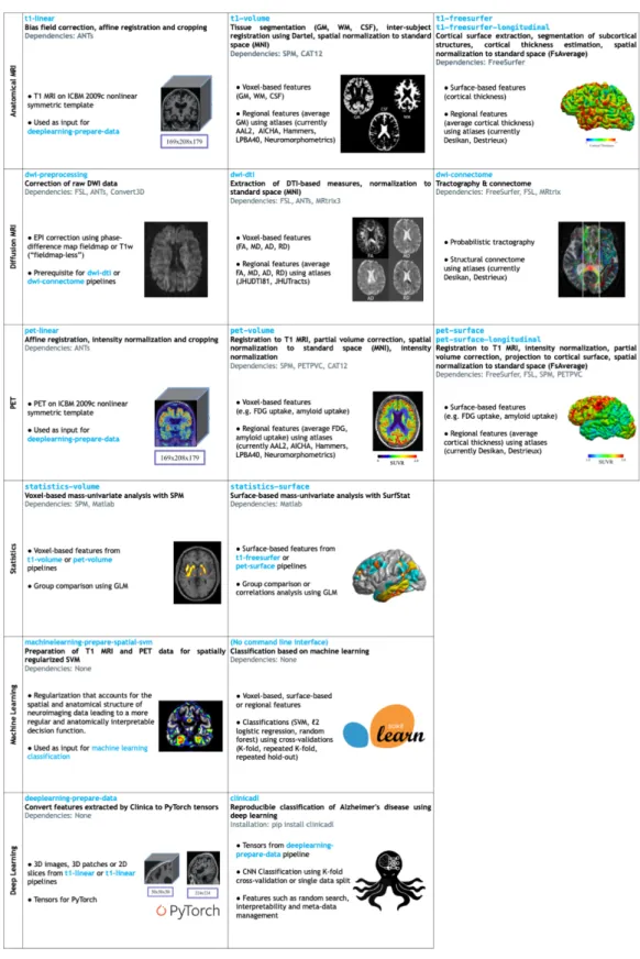
Figure 2 List of the pipelines currently available in Clinica with their dependencies and outputs.
299
Explanations regarding the atlases can be found in section 3.5. GM: gray matter; CSF: cerebrospinal 300
fluid; WM: white matter; FA: fractional anisotropy; MD: mean diffusivity; AD: axial diffusivity; RD: 301
radial diffusivity, SVM: Support Vector Machine; ICBM: International Consortium for Brain 302
Mapping. 303
12
4 Image processing pipelines (clinica run)
305
This section gives a brief description of the different pipelines currently provided by Clinica as well as 306
the types of features Clinica can produce. An illustrative summary of the pipelines can be found in 307
Erreur ! Source du renvoi introuvable..
308
For technical details, we refer the reader to the online user documentation available on the 309
Clinica website where a longer description of each pipeline is provided. 310
4.1 Anatomical MRI
311
4.1.1 Linear processing of T1-weighted MR images (t1-linear)
312
The t1-linear pipeline performs a set of steps in order to affinely align T1w MR images to the MNI 313
space using the ANTs software package (Avants et al., 2014a, 201). These steps include: bias field 314
correction using N4ITK (Tustison et al., 2010); affine registration to the MNI152NLin2009cSym 315
template (Fonov et al., 2009, 2011) in MNI space with the SyN algorithm (Avants et al., 2008a); 316
cropping of the registered images to remove the background. 317
This pipeline was designed to be a prerequisite for the deeplearning-prepare-data 318
pipeline. 319
320
4.1.2 Processing of T1-weighted MR images for volume analyses using SPM (t1-volume*)
321
The t1-volume* pipelines extract voxel-based anatomical features from T1w MR images. 322
Specifically, they perform segmentation of tissues (gray matter (GM), white matter (WM), 323
cerebrospinal fluid (CSF)), normalization to MNI space and computation of regional measures using 324
atlases. Their main outputs are voxel-based maps of tissue density and average measures within cortical 325
regions stored as TSV files. 326
To that purpose, the pipeline wraps the Segmentation, Run Dartel and Normalise to MNI Space 327
routines implemented in SPM (Ashburner, 2012). First, the Unified Segmentation procedure 328
(Ashburner and Friston, 2005) is used to simultaneously perform tissue segmentation, bias field 329
correction and spatial normalization of the input image. Next, a group template is created using 330
DARTEL, an algorithm for diffeomorphic image registration (Ashburner, 2007), from the subjects’ 331
tissue probability maps on the native space, usually GM, WM and CSF, obtained at the previous step. 332
The DARTEL to MNI method (Ashburner, 2007) is then applied, providing a registration of the native 333
space images into the MNI space. 334
335
4.1.3 Processing of T1-weighted MR images for surface analyses using FreeSurfer (t1-freesurfer;
336
t1-freesurfer-longitudinal)
337
The t1-freesurfer pipeline is mainly a wrapper of the recon-all tool of FreeSurfer (Fischl, 338
2012). It performs segmentation of subcortical structures (Fischl et al., 2002, 2004a), extraction of 339
cortical surfaces, cortical thickness estimation (Fischl and Dale, 2000), spatial normalization onto the 340
FreeSurfer surface template (FsAverage) (Fischl et al., 1999), and parcellation of cortical regions using 341
the Desikan and Destrieux atlases (Fischl et al., 2004b). Its main outputs are surface-based cortical 342
thickness features and regional statistics (e.g. regional volume, mean cortical thickness). 343
13
The t1-freesurfer-longitudinal pipeline processes a series of images acquired at 344
different time points for the same subject with the longitudinal FreeSurfer stream (Reuter et al., 2012) 345
to increase the accuracy of volume and thickness estimates. It does so in a single command consisting 346
of two consecutive steps: 1) within-subject template creation (recon-all -base command) to 347
produce an unbiased template image from the different time points using robust and inverse consistent 348
registration (Reuter et al., 2010); 2) longitudinal correction (recon-all -long command): 349
segmentation, surface extraction and computation of measurements at each time point. 350
351
4.2 Diffusion MRI
352
4.2.1 DWI pre-processing (dwi-preprocessing-*)
353
The dwi-preprocessing-* pipelines correct diffusion-weighted MRI (DWI) datasets for motion, 354
eddy current, magnetic susceptibility and bias field distortions, assuming that the data have been 355
acquired using an echo-planar imaging (EPI) sequence. 356
Due to the heterogeneity in acquisitions of fieldmaps and techniques to correct magnetic 357
susceptibility distortions, several pipelines are proposed. Currently, Clinica can handle DWI datasets 358
with fieldmap data containing a phase-difference map (case ‘phase-difference map and at least one 359
magnitude image’ in the BIDS specifications18) (dwi-preprocessing-using-fmap) and DWI
360
datasets with no extra data (dwi-preprocessing-using-t1), which is the case of the public 361
Alzheimer’s Disease Neuroimaging Initiative (ADNI)19 dataset for instance.
362
In all cases, motion and eddy motion corrections are performed with the FSL software 363
(Jenkinson et al., 2012) using the eddy tool (Andersson and Sotiropoulos, 2016) with the replace 364
outliers (--repol) option (Andersson et al., 2016) while bias field is corrected with the ANTs N4 bias 365
correction (Tustison et al., 2010). Regarding susceptibility correction, the FSL prelude/fugue tools 366
were used for the dwi-preprocessing-using-fmap pipeline and the ANTs SyN registration 367
algorithm (Leow et al., 2007; Avants et al., 2008a) for the dwi-preprocessing-using-t1 pipeline. 368
The outputs of the pipelines are the corrected DWI datasets and a brain mask of the b=0 image. 369
These pipelines are prerequisites for the dwi-dti and dwi-connectome pipelines. 370
371
4.2.2 Computation of DTI, DTI-scalar maps and ROI analysis (dwi-dti)
372
The dwi-dti pipeline extracts voxel-based features from diffusion tensor imaging (DTI), namely the 373
fractional anisotropy (FA), mean diffusivity (MD), axial diffusivity (AD) and radial diffusivity (RD) 374
using MRtrix3 (Tournier et al., 2012). Then, the DTI-derived scalar maps (FA, MD, AD, RD) are 375
normalized with ANTs (Avants et al., 2008a) onto an FA-atlas with labelled tracts. Its main outputs 376
are voxel-based maps from DTI and average measures within tracts stored as TSV files. 377
378
18http://bids.neuroimaging.io/ 19http://adni.loni.usc.edu/
14
4.2.3 Computation of fiber orientation distributions, tractogram and structural connectome
379
(dwi-connectome)
380
The dwi-connectome pipeline computes a weighted graph encoding anatomical connections between 381
a set of brain regions from corrected DWI datasets. To that aim, it relies on the MRtrix3 (Tournier et 382
al., 2012) software to compute the constrained spherical deconvolution diffusion model (Tournier et 383
al., 2007), perform probabilistic tractography (Tournier et al., 2010) and computes a connectome using 384
the Desikan & Destrieux atlases from FreeSurfer (Fischl, 2012). Its main outputs are the diffusion 385
model, the whole-brain tractography and the connectivity matrices. 386
387
4.3 Positron emission tomography
388
Currently, Clinica is supporting amyloid and FDG PET data but other tracers will be added in the 389
future. 390
4.3.1 Linear processing of PET images (pet-linear)
391
The pet-linear pipeline performs a spatial normalization to the MNI space and intensity 392
normalization of PET images. The first step of the pipeline is an affine registration to the 393
MNI152NLin2009cSym template (Fonov et al., 2009, 2011) in MNI space with the SyN algorithm 394
(Avants et al., 2008b) from the ANTs software package (Avants et al., 2014b). Then, the registered 395
image intensity is normalized using the mean intensity in reference regions resulting in a standardized 396
uptake value ratio (SUVR) map. The normalized imaged is finally cropped to remove the background. 397
398
4.3.2 Processing of PET images for volume analyses (pet-volume)
399
The pet-volume pipeline extracts voxel-based features from PET data. Specifically, it performs intra-400
subject registration of the PET image into the space of the subject’s T1w MR image using SPM 401
(Ashburner, 2012). Optionally, partial volume correction (PVC) can be applied thanks to the PETPVC 402
toolbox (Thomas et al., 2016). Then, inter-subject spatial normalization of the PET image into MNI 403
space is performed based on the DARTEL deformation model of SPM (Ashburner, 2007) and intensity 404
normalization is done using the average PET uptake in a reference region resulting in a SUVR map. 405
Its main outputs are voxel-based maps of SUVR and average measures within cortical regions. 406
407
4.3.3 Processing of PET images for surface analyses (pet-surface; pet-surface-longitudinal)
408
The pet-surface pipeline extracts the PET signal and projects it onto the cortical surface using the 409
approach described in (Marcoux et al., 2018). More precisely, it performs co-registration of PET and 410
T1w MRI, intensity normalization, PVC with the PETPVC toolbox (Thomas et al., 2016), robust 411
projection of the PET signal onto the subject’s cortical surface, parcellation of the cortical regions 412
using the Desikan and Destrieux atlases and spatial normalization onto the FreeSurfer (Fischl, 2012) 413
surface template (FsAverage). Its main outputs are surface-based PET uptake and regional statistics 414
(mean PET uptake) stored as TSV files. 415
15
The pet-surface-longitudinal pipeline performs the same steps as the pet-surface 416
pipeline except that the cortical and white surfaces are estimated with the longitudinal pipeline of 417
FreeSurfer (Reuter et al., 2012). 418
419
4.4 Statistics
420
4.4.1 Voxel-based mass-univariate analysis with SPM (statistics-volume)
421
The statistics-volume pipeline performs statistical analysis on volume-based features using the 422
general linear model (GLM) and random field theory (Worsley et al., 2009). To that aim, the pipeline 423
wraps the statistical analysis toolbox implemented in SPM. Volume-based measurements can be gray 424
matter maps from the t1-volume pipeline or PET measurements from the pet-volume pipeline. 425
Currently, statistical analysis includes only group comparison. 426
427
4.4.2 Surface-based mass-univariate analysis with SurfStat (statistics-surface)
428
The statistics-surface pipeline performs statistical analysis on surface-based features using the 429
GLM. To that aim, the pipeline relies on the Matlab toolbox SurfStat designed for statistical analyses 430
of univariate and multivariate surface and volumetric data using the GLM (Worsley et al., 2009). 431
Surface-based measurements are analyzed on the FsAverage surface template from FreeSurfer. The 432
pipeline can handle cortical thickness from the t1-freesurfer pipeline or PET measurements from 433
the pet-surface pipeline. Currently, statistical analysis includes group comparison and correlation. 434
435
4.5 Machine Learning
436
4.5.1 Classification based on machine learning (no command line)
437
Clinica provides a modular way to perform classification based on machine learning. To build their 438
own classification pipeline, the user can combine three modules based on the scikit-learn library 439
(Pedregosa et al., 2011): 440
- Input module. The user can select the inputs from the features available in the CAPS directory, 441
such as gray matter maps obtained from T1w MR images, or SUVR maps obtained from FDG 442
PET images. 443
- Algorithm module. The user can choose between different classifiers, currently support vector 444
machine (SVM), logistic regression and random forest. 445
- Validation module. Several cross-validation (CV) methods are available: k-fold CV, repeated 446
k-fold CV and repeated hold-out CV. 447
Note that no command line interface is available for these specific tools. 448
16
More details regarding the different modules and a description of the way they can be used to 449
perform reproducible evaluation of classification methods in Alzheimer’s disease can be found in 450
(Samper-González et al., 2018) and its dedicated repository20.
451 452
4.5.2 Spatially-regularized support vector machine (machinelearning-prepare-spatial-svm)
453
The machinelearning-prepare-spatial-svm pipeline allows the preparation of T1w MRI and 454
PET data to perform classification with an SVM with spatial and anatomical regularization (Cuingnet 455
et al., 2013). In this approach, the standard regularization of the SVM is replaced with a regularization 456
that accounts for the spatial and anatomical structure of neuroimaging data. More specifically, it is 457
regularized with respect to the tissue maps (GM, WM, CSF). As a result, the decision function learned 458
by the algorithm will be more regular and anatomically interpretable. Because the SVM is a kernel 459
method, the spatial/anatomical regularization is done as a pre-processing on the feature maps and the 460
result can then be fed to a standard linear SVM. 461
462
4.6 Deep Learning
463
4.6.1 Prepare data for deep learning (deeplearning-prepare-data)
464
The deeplearning-prepare-data pipeline allows the preparation of data for subsequent training 465
or inference of deep learning models. To that aim, it uses the outputs from t1-linear or pet-linear 466
pipelines. Specifically, 3D images, 3D patches or 2D slices can be extracted and converted into 467
PyTorch tensors (Paszke et al., 2019). 468
469
4.6.2 Training and validation of deep learning models (clinicadl)
470
The training and validation of deep learning models based on Clinica outputs can be performed using 471
a dedicated Python library: ClinicaDL21. This extension of Clinica contains essential features for deep
472
learning application to 3D medical images: 473
- modules to split data avoiding data leakage, which is a major problem in the domain (Wen et 474
al., 2020); 475
- a training method for autoencoders, CNN and a multi-CNN framework which allows the use 476
of other networks trained with ClinicaDL for transfer learning; 477
- a testing function to evaluate the performance of classifiers on independent test sets; 478
- saliency maps generation (Simonyan et al., 2013) extensively used to interpret the outputs of 479
deep learning networks; 480
- basic network architecture search tools, such as random search utilities and methods to generate 481
trivial synthetic datasets for architecture debugging. 482
20https://github.com/aramis-lab/AD-ML 21https://github.com/aramis-lab/AD-DL
17
This library is documented in an independent documentation22. An online tutorial23 allows beginners
483
to better understand these functionalities by testing them locally, or on Google Colab if they do not 484
have access to sufficient computational resources. 485
486
5 Clinica utilities
487
5.1 Conversion of neuroimaging datasets into a BIDS hierarchy (clinica convert)
488
Clinica provides tools to curate several publicly available neuroimaging datasets and automatically 489
convert them into the BIDS standardized data structure. This section explains what the user needs to 490
download prior to running the converter and the rationale behind the selection of data when multiple 491
acquisitions or pre-processing steps are available. For all converters, the user only needs to download 492
the dataset. All subsequent conversion steps are performed automatically (no user intervention is 493
required) and use parallelization for faster processing. For further details, the reader can refer to 494
(Samper-González et al., 2018). 495
496
5.1.1 Conversion of the ADNI dataset to BIDS (adni-to-bids)
497
The ADNI to BIDS converter requires the user to have downloaded all the ADNI study data (tabular 498
data in CSV format) and the imaging data of interest. Note that the downloaded files must be kept 499
exactly as they were downloaded. The imaging modalities currently being converted to BIDS include 500
T1w MRI, FLAIR, DWI, fMRI, FDG PET, PiB PET, Florbetapir (AV45) PET and Flortaucipir 501
(AV1451) PET. Clinical data are also converted to BIDS. They include data that do not change over 502
time, such as the subject’s sex, education level or diagnosis at baseline, as well as session-dependent 503
data, such as the clinical scores. The clinical data being converted are defined in a spreadsheet that is 504
available with the code of the converter. The user can easily modify this file if they want to convert 505
additional clinical data. 506
507
5.1.2 Conversion of the AIBL dataset to BIDS (aibl-to-bids)
508
The AIBL to BIDS converter requires the user to have downloaded the AIBL non-imaging data (tabular 509
data in CSV format) and the imaging data of interest. For each AIBL participant, the T1w MRI and the 510
Florbetapir, PiB and Flutemetamol PET images are converted. As for the ADNI converter, clinical data 511
converted to BIDS are defined in a spreadsheet available with the code of the converter, which the user 512
can modify. 513
514
5.1.3 Conversion of the NIFD dataset to BIDS (nifd-to-bids)
515
The NIFD to BIDS converter requires the user to have downloaded the NIFD imaging data alongside 516
the corresponding clinical data in CSV format. For each NIFD participant, the T1w MRI, FLAIR, PiB 517
22https://clinicadl.readthedocs.io/en/latest/
18
PET and FDG PET images are converted. The clinical data conversion is as described in the previous 518
sections. 519
520
5.1.4 Conversion of the OASIS dataset to BIDS (oasis-to-bids)
521
The OASIS to BIDS converter requires the user to have downloaded the OASIS-1 imaging data and 522
the associated CSV file. For each subject, among the multiple T1w MR images available, we select the 523
average of the motion-corrected co-registered individual images resampled to 1 mm isotropic voxels. 524
The clinical data are converted as described in the previous sections. 525
526
5.1.5 Syntax to run the converters
527
After having downloaded the clinical and imaging data of one of these studies, the conversion of a 528
dataset into BIDS is performed using the following syntax: 529
clinica convert <dataset>-to-bids dataset_directory clinical_data_directory 530
bids_directory 531
where <dataset>-to-bids can be adni-to-bids, aibl-to-bids, nifd-to-bids or oasis-532
to-bids. 533
534
5.2 Data handling tools (clinica iotools)
535
We also propose a set of tools that allows the user to handle BIDS and CAPS datasets. For the moment, 536
there are five different commands: 537
- center-nifti: Center Nifti files of a BIDS directory. 538
- check-missing-modalities: This command checks missing modalities in a BIDS 539
directory. 540
- check-missing-processing: This command checks the outputs in a CAPS directory. 541
- create-subjects-visits: This command generates a list of subjects with their sessions 542
based on a BIDS directory and stores the outputs in a TSV file. 543
- merge-tsv: This command merges all the tabular data including the clinical data of a BIDS 544
directory and the regional features from a CAPS directory (e.g. mean GM density in AAL2 545
atlas) into a single TSV file. This file can then be easily plugged into machine learning tools 546
via Clinica or other statistical/machine learning software packages. 547
19
6 Usage example
549
In this section, we propose to show how Clinica can be used to perform a group comparison of FDG 550
PET data projected on the cortical surface between patients with Alzheimer’s disease and healthy 551
controls from the ADNI database. An illustrative summary of this example can be found in Figure 3. 552
To download the ADNI dataset, it is necessary to register to the LONI Image & Data Archive24,
553
a secure research data repository, and request access to the ADNI dataset through the submission of an 554
online application form. Both the imaging and clinical data need to be downloaded, each to a folder 555
that we will call imaging_data_dir and clinical_data_dir, respectively. The following 556
command can be used to convert the T1 and FDG PET data of the ADNI dataset into BIDS: 557
clinica convert adni-to-bids imaging_data_dir clinical_data_dir ADNI_BIDS 558
--modalities T1 PET_FDG 559
where the ADNI_BIDS folder contains the conversion of ADNI into BIDS. We can now start processing 560
the data. First, we need to extract the cortical surfaces from each anatomical image. To do so, we simply 561
need to type on the terminal the following command: 562
clinica run t1-freesurfer ADNI_BIDS ADNI_CAPS 563
where the output data will be stored in the ADNI_CAPS folder. After visual inspection of the generated 564
outputs, the FDG PET data can be projected onto the cortex. The command line will be: 565
clinica run pet-surface ADNI_BIDS ADNI_CAPS fdg pons pvc_psf.tsv 566
where fdg is the label given to the PET acquisition, pons is the reference region for the SUVR map 567
computation and pvc_psf.tsv is the TSV file containing PSF information for each PET image. 568
Finally, we can perform group comparison of cortical FDG PET data after having checked the outputs. 569
The demographic information of the population studied will be stored in a TSV file, looking as follows: 570
participant_id session_id group age sex 571
sub-ADNI094S2201 ses-M00 HC 63.7 Female 572
sub-ADNI098S4018 ses-M00 HC 76.1 Male 573
sub-ADNI023S4020 ses-M00 HC 66.5 Male 574
sub-ADNI031S4021 ses-M00 HC 66.5 Male 575
sub-ADNI094S1397 ses-M00 AD 55.1 Female 576
sub-ADNI094S1402 ses-M00 AD 69.3 Male 577
sub-ADNI128S1409 ses-M00 AD 65.9 Male 578
sub-ADNI128S1430 ses-M00 AD 83.4 Female 579
... 580
where participants with Alzheimer’s disease (respectively healthy controls) have the AD label 581
(respectively HC label) in the group column. We will call this file ADvsHC_participants.tsv. 582
Using age and sex as covariates, the command line will be: 583
20
clinica run statistics-surface ADNI_CAPS ADvsHC pet-surface \ 584
group_comparison ADvsHC_participants.tsv group –covariates "age + sex" 585
The results of the statistical analysis will be stored in the ADNI_CAPS/groups/group-586
ADvsHC folder. 587
21
588
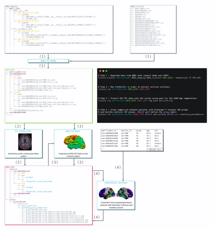
Figure 3 Diagram illustrating the Clinica pipelines involved when performing a group comparison of
589
FDG PET data projected on the cortical surface between patients with Alzheimer’s disease and healthy 590
controls from the ADNI database. First, clinical and neuroimaging data are downloaded from the ADNI 591
website and data are converted into BIDS with the adni-to-bids tool from Clinica (1). Estimation 592
of the cortical and white surface is then produced by the t1-freesurfer pipeline in a single 593
command line (2). Afterwards, FDG PET data can be projected on the subject’s cortical surface and 594
normalized to the FsAverage template from FreeSurfer using the pet-surface pipeline (3). Finally, 595
a TSV file with demographic information of the population studied is given to the statistics-596
surface pipeline to generate the results of the group comparison between patients with Alzheimer’s 597
disease and healthy controls (4). 598
22
7 Discussion
599
We proposed a software platform that aims at making clinical neuroscience easier and more 600
reproducible. Clinica automates the processing of pipelines involving several neuroimaging modalities 601
(currently, anatomical MRI, diffusion MRI, and PET) as well as statistics, machine learning and deep 602
learning tools. Additionally, Clinica provides tools to convert public neuroimaging datasets focused on 603
dementia (ADNI, AIBL, OASIS and NIFD) into the BIDS standard, and tools to handle raw (BIDS) 604
and processed datasets. The use of the BIDS standard as the only prerequisite on the data and the 605
unified command line interface across the pipelines ease the processing automation. The image analysis 606
automation is also improved by the use of the CAPS hierarchy, which facilitates the chaining of 607
pipelines. The target audience of Clinica is neuroscientists or clinicians conducting clinical 608
neuroscience studies involving multimodal imaging, and researchers developing advanced machine or 609
deep learning algorithms. 610
The last three decades witnessed the development of many software packages for the processing 611
of neuroimaging data. A first category of packages comprises those implementing innovative image 612
processing methodologies (e.g. tissue segmentation, registration). Many tools fall into this category, 613
for instance SPM (Friston et al., 2007), AFNI (Cox, 1996), FreeSurfer (Fischl, 2012), FSL (Jenkinson 614
et al., 2012), PETPVC (Thomas et al., 2016), Camino (A Cook et al., 2005), Dipy (Garyfallidis et al., 615
2014), DTI-TK25, MRtrix (Tournier et al., 2012) or ANTs (Avants et al., 2014a). Some of these tools
616
cover a variety of modalities while others focus on a specific one (diffusion MRI for Camino, Dipy, 617
DTI-TK and MRtrix, fMRI for AFNI, PET for PETPVC). However, performing a multimodal study 618
can be difficult because one needs to combine tools from different packages. This results in complex 619
pipelines which can be difficult to build, maintain and distribute. Even when analyzing a single 620
modality, one often wants to combine tools from different packages, thus facing similar difficulties. 621
Combination of tools is made even more difficult by the fact that the input and output data are organized 622
differently by each tool. 623
Efforts of the community have alleviated several of these difficulties. The NeuroDebian 624
community26 (Halchenko and Hanke, 2012) aims to provide and ease the installation of a large
625
collection of software packages for the Debian distribution. The Nipype (Gorgolewski et al., 2011) 626
system facilitates the building of complex pipelines through the wrapping of tools in Python. BIDS 627
(Gorgolewski et al., 2017) provides a standard for organizing data. BIDS-Apps provides versions of 628
software packages using BIDS for data organization. More generally, the NIPY community aims to 629
provide a comprehensive set of tools for the analysis of neuroimaging data in a single language, Python. 630
However, many useful tools and packages remain outside of the NIPY scope, being written in different 631
languages. As mentioned above, Nipype allows wrapping these heterogeneous tools. It is a powerful 632
and particularly useful tool for that aim. However, the building of pipelines remains left to the user. 633
This requires substantial development efforts. Clinicians/neuroscientists often do not have the 634
necessary programming expertise, while researchers in machine learning often do not have the 635
necessary neuroimaging expertise. Therefore, Nipype and Clinica do not have the same objectives. 636
Nipype provides a powerful way to write pipelines. As such, it is particularly flexible but requires some 637
programming expertise. Clinica, on the other hand, offers a set of predefined pipelines: it is thus easier 638
to use but less flexible. 639
25http://dti-tk.sourceforge.net 26http://neuro.debian.net/
23
There are also software packages that integrate different tools within a single environment. This 640
is for example the case of BCBtoolkit (Foulon et al., 2018), BrainVISA (Cointepas et al., 2001), 641
BrainSuite27, fMRIPrep (Esteban et al., 2019), or Pypes (Savio et al., 2017). Clinica falls within this
642
category. It shares some characteristics with these tools but also has important differences. The 643
BCBtoolkit wraps neuroimaging software packages from the community but also highlights new 644
methodological developments to evaluate brain disconnections. BCBoolkit does not use any pipelining 645
system but instead wraps bash scripts that are then made available through a GUI. The BrainVISA 646
platform, even though it also wraps some existing tools, mainly provides innovative tools for the 647
analysis of human or animal brain imaging data. Moreover, it includes its own pipelining system while 648
Clinica relies on the community effort Nipype. BrainSuite does not wrap existing tools but provides a 649
set of innovative tools for the analysis of neuroimaging data. It can be executed using a GUI, a 650
command line, a Nipype interface, or as a BIDS App. fMRIPrep combines software components using 651
Nipype (Gorgolewski et al., 2011) to provide a robust pipeline for pre-processing of fMRI data. It 652
assumes input data to follow the BIDS standard (Gorgolewski et al., 2016) and outputs are organized 653
following the ongoing BIDS-derivatives initiative. Pypes is probably the closest in spirit to Clinica: it 654
also focuses on the integration of existing tools into a set of reusable pipelines built with Nipype. The 655
user needs to specify a configuration file to describe the input data even for BIDS datasets. The output 656
data will then follow the same structure as the input data and can be chained to other pipelines from 657
Pypes. Note that the ability to chain pipelines exists for a limited number of pipelines in the BIDS-App 658
version of BrainSuite and is likely to be more present in BIDS Apps with the advent of BIDS-659
derivatives. Although Clinica does not provide a GUI, efforts were made to simplify as much as 660
possible its command line interface, which is feasible thanks to the autocompletion, the structured 661
organization of data and the documentation which was designed in order to be readable by a newcomer. 662
Machine learning is now widely used in the neuroimaging community, for cognitive 663
neuroscience or computer-aided diagnosis applications. However, applying such approaches to 664
neuroimaging data can be difficult for newcomers. Conversely, researchers in machine learning are 665
often interested in applying and validating their approaches to clinical neuroimaging problems (e.g. 666
diagnosis, prognosis). However, they often lack the necessary knowledge for preprocessing 667
neuroimaging data and extracting features. Nilearn (Abraham et al., 2014) has allowed major progress 668
in that direction by providing in a single environment tools for preprocessing, data manipulation, 669
feature extraction and machine learning wrapping the scikit-learn library (Pedregosa et al., 2011). 670
However, Nilearn currently mostly targets cognitive neuroimaging and mainly deals with functional 671
neuroimaging. On the other hand, Clinica is dedicated to clinical neuroimaging studies, such as 672
biomarker design and clinical decision support systems. As a result, Clinica does not aim to deal with 673
task-based fMRI and is currently mostly focused on the analysis of T1w MRI, diffusion MRI and PET 674
data. Deep learning methods are also increasingly applied to neuroimaging. Even though such methods 675
usually do not rely on pre-extracted features, they will still require some preprocessing and data 676
conversion tools in order to use neuroimaging data in frameworks such as PyTorch. Clinica provides 677
such tools. 678
Reproducibility has been highlighted as a major challenge in many scientific fields including 679
neuroimaging (Poldrack et al., 2017). This problem has also been highlighted in machine learning for 680
healthcare in general (McDermott et al., 2019) and for brain diseases in particular (Samper-González 681
et al., 2018; Wen et al., 2021). Clinica aims to make reproducible research easier to perform. To that 682
purpose, it combines: 1) use of a community standard for inputs; 2) the definition of a standardized 683
organization for outputs; 3) standardized ways to extract features; 4) extensive software testing. As 684
24
previously mentioned, it extensively relies on community achievements such as the BIDS standard and 685
Nipype. 686
Clinica currently has the following limitations. First, we will improve the enforcement of 687
reproducibility by adding traceability features. Furthermore, quality control (QC) of processed data is 688
currently done using standard image viewers which is clearly suboptimal. We plan to add more 689
advanced QC of outputs in the spirit for instance of MindControl (Keshavan et al., 2018). Finally, new 690
longitudinal analysis pipelines (beyond those already present for FreeSurfer and PET surface 691
processing) will be developed. 692
25
8 Conflict of Interest
694
The authors declare that the research was conducted in the absence of any commercial or financial 695
relationships that could be construed as a potential conflict of interest. 696
9 Author Contributions
697
Study concepts/study design, all authors; manuscript drafting or manuscript revision for important 698
intellectual content, all authors; approval of final version of submitted manuscript, all authors; literature 699
research, AR, NB, OC; and manuscript editing, all authors. 700
10 Funding
701
The research leading to these results has received funding from the programs “Investissements 702
d’avenir” ANR-10-IAIHU-06 (Agence Nationale de la Recherche-10-IA Institut Hospitalo-703
Universitaire-6), ANR-11-IDEX-004 (Agence Nationale de la Recherche-11- Initiative d’Excellence-704
004, project LearnPETMR number SU-16-R-EMR-16) and ANR-19-P3IA-0001 (PRAIRIE 3IA 705
Institute), from the European Union H2020 program (project EuroPOND, grant number 666992, 706
project HBP SGA1 grant number 720270), from the joint NSF/NIH/ANR program “Collaborative 707
Research in Computational Neuroscience” (project HIPLAY7, grant number ANR-16-NEUC-0001-708
01), from Agence Nationale de la Recherche (project PREVDEMALS, grant number ANR-14-CE15-709
0016-07), from the ICM Big Brain Theory Program (project DYNAMO), from the Inria Project Lab 710
Program (project Neuromarkers), from the European Research Council (to Dr Durrleman project 711
LEASP, grant number 678304), and from the “Contrat d’Interface Local” program (to Dr Colliot) from 712
Assistance Publique-Hôpitaux de Paris (AP-HP). N.B. received funding from the People Programme 713
(Marie Curie Actions) of the European Union’s Seventh Framework Programme (FP7/2007-2013) 714
under REA grant agreement no. PCOFUND-GA-2013-609102, through the PRESTIGE programme 715
coordinated by Campus France. 716