Comparing elliptic and toric hypersurface
Calabi-Yau threefolds at large Hodge numbers
The MIT Faculty has made this article openly available.
Please share
how this access benefits you. Your story matters.
Citation
Huang, Yu-Chien, and Washington Taylor. “Comparing Elliptic
and Toric Hypersurface Calabi-Yau Threefolds at Large Hodge
Numbers.” Journal of High Energy Physics, vol. 2019, no. 2, Feb.
2019. © The Authors
As Published
https://doi.org/10.1007/JHEP02(2019)087
Publisher
Springer Berlin Heidelberg
Version
Final published version
Citable link
http://hdl.handle.net/1721.1/120533
Terms of Use
Creative Commons Attribution
JHEP02(2019)087
Published for SISSA by SpringerReceived: August 13, 2018 Revised: December 29, 2018 Accepted: January 22, 2019 Published: February 14, 2019
Comparing elliptic and toric hypersurface Calabi-Yau
threefolds at large Hodge numbers
Yu-Chien Huang and Washington Taylor
Center for Theoretical Physics, Department of Physics, Massachusetts Institute of Technology, 77 Massachusetts Avenue, Cambridge, MA 02139, U.S.A.
E-mail: yc huang@mit.edu,wati@mit.edu
Abstract: We compare the sets of Calabi-Yau threefolds with large Hodge numbers that are constructed using toric hypersurface methods with those can be constructed as elliptic fibrations using Weierstrass model techniques motivated by F-theory. There is a close correspondence between the structure of “tops” in the toric polytope construction and Tate form tunings of Weierstrass models for elliptic fibrations. We find that all of the Hodge number pairs (h1,1, h2,1) with h1,1 or h2,1≥ 240 that are associated with threefolds in the Kreuzer-Skarke database can be realized explicitly by generic or tuned Weierstrass/Tate models for elliptic fibrations over complex base surfaces. This includes a relatively small number of somewhat exotic constructions, including elliptic fibrations over non-toric bases, models with new Tate tunings that can give rise to exotic matter in the 6D F-theory picture, tunings of gauge groups over non-toric curves, tunings with very large Hodge number shifts and associated nonabelian gauge groups, and tuned Mordell-Weil sections associated with U(1) factors in the corresponding 6D theory.
Keywords: Differential and Algebraic Geometry, F-Theory, Superstring Vacua ArXiv ePrint: 1805.05907
JHEP02(2019)087
Contents
1 Introduction 1
2 F-theory physics and elliptic Calabi-Yau threefold geometry 3 2.1 Hodge numbers and the 6D massless spectrum 4 2.2 Generic and tuned Weierstrass models for elliptic Calabi-Yau manifolds 5
2.3 Tate form and the Tate algorithm 8
2.4 The Zariski decomposition 11
2.5 Zariski decomposition of a Tate tuning 12 2.6 Matter content from anomaly constraints in F-theory 14 2.7 Global symmetry constraints in F-theory 16
2.8 Base surfaces for 6D F-theory models 17
3 Elliptic fibrations in the toric reflexive polytope construction 18
3.1 Brief review of toric varieties 18
3.2 Batyrev’s construction of Calabi-Yau manifolds from reflexive polytopes 19
3.3 Fibered polytopes in the KS database 21
3.4 Standard P2,3,1-fibered polytopes and corresponding Tate models 23 3.5 A method for analyzing fibered polytopes: fiber types and 2D toric bases 25 4 Tate tunings and the Kreuzer-Skarke database 28 4.1 Reflexive polytopes from elliptic fibrations without singular fibers 29
4.2 Tate tuning and polytope tops 31
4.3 Reflexive polytopes for NHCs and Tate tunings 35 4.3.1 NHCs with immediately reflexive polytopes 35 4.3.2 Other NHCs: reflexive polytopes from the dual of the dual 36 4.3.3 Reflexive polytopes from Tate tunings 37
4.4 Multiple tops 38
4.5 Combining tunings 42
4.6 Tate tunings and polytope models of so(n) gauge algebras 45
4.7 Multiplicity in the KS database 48
4.8 Bases with large Hodge numbers 51
5 Systematic construction of Tate-tuned models in the KS database 53 5.1 Algorithm: global symmetries and Zariski decomposition for Weierstrass
models 54
5.2 Main structure of the algorithm: bases with a non-Higgsable e7 or e8 55
5.3 Special cases: bases lacking curves of self-intersection m ≤ −7 and/or having curves of non-negative self intersection 58
JHEP02(2019)087
6 Polytope analysis for cases missing from the simple tuning construction,
and other exotic constructions 61
6.1 Fibered polytope models with Tate forms 62 6.1.1 Type I2ns Tate tunings and exotic matter 62
6.1.2 Large Hodge number shifts 65
6.1.3 Tate-tuned models corresponding to non-toric bases 67 6.2 Weierstrass models from non-standard P2,3,1-fibered polytopes 69
6.2.1 A warmup example 72
6.2.2 The eight remaining missing cases at large h1,1 74 6.2.3 Example: a model with a tuned genus one curve in the base 78
7 Conclusions 79
7.1 Summary of results 79
7.2 Possible extensions of this work 80
A Standard P2,3,1-fibered polytope tuning 81 B Elliptic fibrations over the bases F9, F10, and F11 83
C An example with a nonabelian tuning that forces a U(1) factor 85
1 Introduction
While Calabi-Yau threefolds have played an important role in string theory since the early days of the subject [1], the set of these geometries is still relatively poorly understood. Following the approach of Batyrev [2], in 2000 Kreuzer and Skarke carried out a complete analysis of all reflexive polytopes in four dimensions, giving a systematic classification of those Calabi-Yau (CY) threefolds that can be realized as hypersurfaces in toric varieties [3]. For many years the resulting database [4] has represented the bulk of the known set of Calabi-Yau threefolds, particularly at large Hodge numbers. More recently, the study of F-theory [5–7] has motivated an alternative method for the systematic construction of Calabi-Yau threefolds that have the structure of an elliptic fibration (with section). By systematically classifying all bases that support an elliptically fibered CY [8–11] and then systematically considering all possible Weierstrass tunings [12,13] over each such base, it is possible in principle to construct all elliptically fibered Calabi-Yau threefolds. While there are some technical issues that must still be resolved for a complete classification from this approach, at large Hodge numbers this method gives a reasonably complete picture of the set of possibilities. One perhaps surprising result that has recently become apparent both from this work and from other perspectives [14–19] is that a very large fraction of the set of Calabi-Yau threefolds that can be constructed by any known mechanism are actually elliptically fibered, particularly at large Hodge numbers.
JHEP02(2019)087
The goal of this paper is to carry out a direct comparison of the set of elliptically fibered Calabi-Yau threefolds that can be constructed using Weierstrass/Tate F-theory based methods with those that arise through reflexive polytope constructions. While the general methods for construction of elliptic Calabi-Yau threefolds can include non-toric bases [10, 11], and even over toric bases there are non-toric Weierstrass tunings [12,13], we focus here on the subset of constructions that have the potential for a toric description through a reflexive polytope. In section 2, we review some of the basics of F-theory and the systematic construction of elliptic Calabi-Yau threefolds through the geometry of the base and the tuning of Weierstrass or Tate models from the generic structure over each base. In section 3, we review the Batyrev construction and reflexive polytopes, and the structure of elliptic fibrations in this context. In particular, in section 3.4 we describe the precise correspondence between a particular fibration structure for a reflexive polytope and Tate form Weierstrass models. In section4, we restrict attention to toric base surfaces B2 and identify the set of tuned Weierstrass/Tate models over such bases that naturally
correspond to a reflexive polytope in the Batyrev construction. This gives us a systematic way of constructing from the point of view of elliptic fibrations over a chosen base a large set of elliptic Calabi-Yau threefolds that are expected to be seen in the Kreuzer-Skarke database with a specific (P2,3,1) fiber type. At large Hodge numbers, for reasons discussed
further in section 4.8, we expect that this should give most or all elliptic fibrations that arise in the KS database; we find that this is in fact the case.
The main results of the paper are in section 5 and section 6, where we describe an algorithm to systematically run through all tuned Tate models over toric bases and we compare the results of running this algorithm to the Kreuzer-Skarke database. The initial result, described in section5, is that these simply constructed sets match almost perfectly in the large Hodge number regimes that we study: both at large h2,1and at large h1,1all the models constructed by an appropriate set of Tate tunings over toric bases appear in the KS database, and virtually all the Hodge numbers in the database are reproduced by elliptic Calabi-Yau threefolds produced using this approach. There is a small set of large Hodge numbers (18 out of 1,827) associated with toric hypersurface Calabi-Yaus, however, that are not reproduced by our initial scan. By examining these individual cases, as described in section 6, we find that all these exceptions also correspond to elliptic fibrations though with more exotic structure, such as non-flat fibrations resolved through extra blow-ups in the base that take the base outside the toric class, and/or force Mordell-Weil sections on the elliptic fiber. The upshot is that when these more exotic constructions are included, all Hodge number pairs with either h1,1 or h2,1 at least 240 are reproduced by an elliptic
Calabi-Yau over some explicitly determined base surface. We conclude in section 7 with a summary of the results and some related open questions.
Note that in this paper the focus is on understanding in some detail the connection between elliptic fibration geometry and polytope geometry for these different approaches to construction of elliptic Calabi-Yau threefolds. In a companion paper [20] we will describe a more direct analysis of the polytopes in the KS database that also shows explicitly that there is a toric fiber associated with an elliptic fibration for every polytope in the database at large Hodge numbers. The principal class of Tate tunings that we consider in this paper
JHEP02(2019)087
have a complementary description in the language of “tops” [21]. The construction of many polytopes in the KS database through combining K3 tops and “bottoms” was accomplished in [14], and a systematic approach to constructing toric hypersurface Calabi-Yau threefold with a given base and gauge group using the language of tops is developed in [23], with particular application to models with gauge group SU(5) as also studied in e.g. [24, 25]. One of the main results of this paper is the systematic relationship of such constructions with certain classes of Tate tunings. This leads in some cases to the identification of new Tate tunings from observed polytope structures, and the observation that some polytopes in the KS database have a more complex structure that does not admit a direct description in terms of standard tops. On the other hand, new structures of tops are also found through the construction of polytopes via the correspondence with Tate tunings.
2 F-theory physics and elliptic Calabi-Yau threefold geometry
We briefly summarize here how the massless spectrum of a six-dimensional effective theory from F-theory compactification is related to the geometric data of the internal manifold, which is an elliptically fibered Calabi-Yau threefold (CY3) over a two-dimensional base B2 (complex dimensions). F-theory models can then be systematically studied by first
choosing a base B2 and then specifying an elliptic fibration in Weierstrass form over that
base. Further background on F-theory can be found in for example [5–7,26,27].
F-theory compactified on a (possibly singular) elliptically fibered Calabi-Yau threefold X gives a 6D effective supergravity theory. Such a compactification of F-theory is equivalent to M-theory on the resolved Calabi-Yau ˜X in the decompactification limit of M-theory, where in the F-theory picture the resolved components of the elliptic fiber are shrunk to zero size. F-theory can also be thought of as a nonperturbative formulation of type IIB string theory. In this picture the type IIB theory is compactified on the base B2.
In this F-theory description, spacetime filling 7-branes sit at the codimension-one loci in the base where the fibration degenerates. The non-abelian gauge symmetries of the 6D effective theory arise from the seven-branes and can be inferred from the singularity types of the elliptic fibers along the codimension-one loci in the base, according to the Kodaira classification (table2). At the intersections of seven-branes there are localized matter fields that are hypermultiplets in the 6D theory; the representations of the matter fields can be determined from the detailed form of the singularities over the codimension-two points in the base (see e.g. [28–30]). Therefore the physics data can be extracted by studying the singular fibers by means of the Weierstrass models (short form) or the Tate models (long form) of X that we review in sections 2.2and 2.3.1 There can also be abelian gauge
1
The short form Weierstrass model is the most general form for an elliptic Calabi-Yau threefold. The cases discussed in this paper are elliptically fibered Calabi-Yau threefolds that always have a section and therefore in principle admit a short form Weierstrass form realization. There can also be genus one fibered Calabi-Yau threefolds (lacking a global section), which can be related to Weierstrass models of elliptic
Calabi-Yau threefolds through the Jacobian construction (described from the physics perspective in [31,34]).
The physics of these threefolds is more subtle, involving discrete gauge groups [32,33,35–37]. In a few
cases we find it useful to use the Jacobian construction even for cases with a section, giving an explicit transformation to the short Weierstrass form.
JHEP02(2019)087
symmetries, which arise from additional rational sections of the elliptic fibration [6,7]. The study of u(1) symmetries is more subtle in that it relates to the global structure of the fibration, as opposed to non-abelian symmetries where we can just study singular fibers locally. We will see cases with abelian factors in section 6, with a detailed example worked out in appendix C. In section 2.4, we review the Zariski decomposition, which allows us to determine the order of vanishing and consequent gauge group of a Weierstrass or Tate form description of an elliptic fibration, and in section2.5we describe how this method can be applied systematically in the context of Tate tunings. In section 2.6, we review the 6D anomaly cancellation conditions and their connection to the matter content of a 6D theory and the Hodge numbers of the corresponding Calabi-Yau threefold. In section2.7we review the constraints imposed by global symmetry groups on the set of gauge groups that can be supported on curves intersecting a given curve, and we conclude the overview of F-theory in section2.8with a summary of the systematic classification of complex surfaces that can support elliptic Calabi-Yau threefolds and can be used for F-theory compactification. 2.1 Hodge numbers and the 6D massless spectrum
By going to the 5D Coulomb branch after reduction on a circle, the F-/M-theory cor-respondence can be used to relate the geometry of ˜X to the associated 6D supergravity theory [7,38]. In particular, the Hodge numbers, h1,1 and h2,1, of ˜X can be related to the (massless) matter content of the 6D theory:
h1,1( ˜X) = r + T + 2, (2.1) where T is the number of tensor multiplets, which is determined already by the choice of base B2,
T = h1,1(B2) − 1, (2.2)
and r = rabelian+Piri is the total rank of the gauge group,
G = U(1)rabelian× Y
non-abelian factors i
Gi, (2.3)
of the 6D effective theory. We also have
h2,1( ˜X) = Hneutral− 1, (2.4)
where Hneutral is the number of hypermultiplets that are neutral under the Cartan
subal-gebra2 of the gauge group G of the 6D F-theory.
The spectra of 6D theories are constrained by consistency conditions associated with the absence of anomalies, which we describe in further detail in section 2.6. The gravi-tational anomaly cancellation condition (2.33) gives H − V = 273 − 29T , where V is the
2In other words, this counts fields that are neutral matter fields in the 5D M-theory sense but may
transform under the unhiggsed non-abelian factors of the 6D F-theory. Often, matter charged under the non-abelian factors is still charged under the Cartan subalgebra, but for certain representations of some non-abelian groups there can be charged matter that is neutral under the Cartan subalgebra.
JHEP02(2019)087
Rank r Algebras 2 su(3), g2 3 su(4), so(7) 4 so(8), so(9), f4 r ≥5 so(r), so(r + 1)Table 1. Rank preserving tunings: tunings of these four classes of gauge algebras do not change h1,1 or h2,1.
dimension of the gauge group G, and H = Hcharged+ Hneutral is the total number of
hy-permultiplets (separated into neutral and charged matter under the Cartan of the gauge group G). So we have another expression
h2,1( ˜X) = 272 + V − 29T − Hcharged. (2.5)
This is more useful for some of our purposes than equation (2.4). In particular, as we discuss in further detail in the following section, we are interested in studying various specializations (tunings) of a generic elliptically fibered CY3 over a given base B2. The
number of tensors T is fixed for a given base. Thus, if we start with known Hodge numbers h1,1 and h2,1 for the generic elliptic fibration over a given (e.g. toric [9, 39]) base, and specialize/tune to a model with a larger gauge group and increased matter content, then the Hodge numbers of the tuned model can be simply calculated by adding to those of the generic models respectively the shifts
∆h1,1= ∆r, (2.6)
∆h2,1= ∆V − ∆Hcharged. (2.7)
Such a specialization/tuning amounts physically to undoing a Higgsing transition, and the second of these relations simply expresses the physical expectation that the number of matter degrees of freedom that are lost (“eaten”) in a Higgsing transition is equal to the number of gauge bosons lost to symmetry breaking. Note that the data on the right hand sides are associated in general with tuned non-abelian gauge symmetries but also in some special cases involve abelian factors. Note also that the right-hand sides of (2.6) and (2.7) are always non-negative and non-positive respectively for any tuning. In most cases, the gauge group increases in rank and some of the h2,1moduli are used to implement the tuning. In rank-preserving tunings, however, the Hodge numbers do not change (see table 1) — h1,1 of course does not change in a rank-preserving enhancement; h2,1 does not change either in these tunings, as one can check by considering carefully the matter charged under the Cartan subalgebra (cf. footnote 2.)
2.2 Generic and tuned Weierstrass models for elliptic Calabi-Yau manifolds An elliptic fibration with a section over a base B can be described by the Weierstrass model
JHEP02(2019)087
The Calabi-Yau condition on the total space X requires that f, g are sections of O(−4KB),
O(−6KB), where KB is the canonical class of the base. More abstractly, we take the
weighted projective bundle
π : P = PP2,3,1[L
2⊕ L3⊕ O
B] → B, (2.9)
where L = O(−KB) is required by the Calabi-Yau condition and x ∈ OP(2) ⊗ π∗L2, y ∈
OP(3) ⊗ π∗L3, z ∈ O
P(1) and [x : y : z] can be viewed as weighted projective coordinates
of the P2,3,1, while f and g are sections of, to be more precise, π∗L4 and π∗L6 respectively.
Consider an elliptic Calabi-Yau threefold over a complex two-dimensional base B2, so
the divisors in the base are curves. The elliptic fiber becomes singular over the codimension-one loci in the base where the discriminant
∆ = 4f3+ 27g2 (2.10)
vanishes. The type of singular fiber at a generic point along an irreducible component {σ = 0} of the discriminant locus {∆ = 0} is characterized by the Kodaira singularity type, which is determined by the orders of vanishing of f , g, and ∆ in an expansion in σ (see table 2). The physics interpretation is that there are seven-branes on which open strings (and junctions) end located at the discriminant locus, and the resulting gauge symmetries can be determined (up to monodromies) by the type of the singular fiber. The gauge algebras that are further determined by monodromy conditions [29, 44] are those of types In, I0∗, In∗, IV, IV∗, where some factorizability conditions are imposed on the
terms of f, g, ∆ of lowest degrees of vanishing order along {σ = 0}. We summarize these conditions in table 3, in terms of the first non-vanishing sections fi(ζ), gj(ζ), ∆k(ζ) in the
local expansions
f (σ, ζ) = f0(ζ) + f1(ζ)σ + · · · , (2.11)
g(σ, ζ) = g0(ζ) + g1(ζ)σ + · · · , (2.12)
∆(σ, ζ) = ∆0(ζ) + ∆1(ζ)σ + · · · , (2.13)
where {ζ = 0} defines a divisor that intersects {σ = 0} transversely so that σ, ζ together serve as local coordinates on an open patch of base.
A generic Weierstrass model (i.e. with coefficients at a generic point in the moduli space) for an elliptically fibered CY3 over a given base B2corresponds physically to a
maxi-mally Higgsed phase. In the maximaxi-mally Higgsed phase over many bases the gauge group and matter content are still nontrivial. The minimal gauge algebras and matter configuration associated with a given base B2 are carried by non-Higgsable clusters (NHCs) [8], which
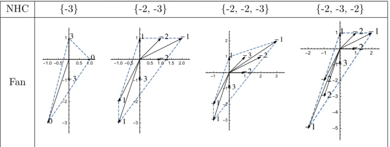
are isolated rational curves of self-intersection m, −12 ≤ m ≤ −3, and clusters of multiple rational curves of self-intersection ≤ −2: {−2, −3}, {−2, −2, −3}, and {−2, −3, −2}. The sections f, g, ∆ automatically vanish to higher orders along these curves in any Weierstrass model over the given base. This can be understood geometrically as an effect in which the curvature over the negative self-intersection curves must be cancelled by 7-branes to maintain the Calabi-Yau structure of the elliptic fibration. The orders of vanishing and the corresponding minimal gauge groups on these NHCs are listed in table 11 in section 4.4.
JHEP02(2019)087
Type ord (f ) ord (g) ord (∆) singularity nonabelian symmetry algebra
I0 ≥ 0 ≥ 0 0 none none In 0 0 n ≥ 2 An−1 su(n) or sp(bn/2c) II ≥ 1 1 2 none none III 1 ≥ 2 3 A1 su(2) IV ≥ 2 2 4 A2 su(3) or su(2) I0∗ ≥ 2 ≥ 3 6 D4 so(8) or so(7) or g2 In∗ 2 3 n ≥ 7 Dn−2 so(2n − 4) or so(2n − 5) IV∗ ≥ 3 4 8 E6 e6 or f4 III∗ 3 ≥ 5 9 E7 e7 II∗ ≥ 4 5 10 E8 e8
non-min ≥ 4 ≥ 6 ≥ 12 does not occur in F-theory
Table 2. Kodaira classification of singularities in the elliptic fiber along codimension one loci in the base in terms of orders of vanishing of the parameters f, g in the Weierstrass model (2.8) and the discriminant locus ∆.
ord(f ) ord(g) ord(∆) algebra monodromy condition
In 0 0 n
su(n)
since ∆0= 0, locally
f0(ζ) = −13u20 and g0(ζ) = 272u30
for some u0(ζ), which is a perfect square sp(bn/2c) otherwise
IV ≥ 2 2 4 su(3) g2(ζ) is a perfect square
su(2) otherwise
I0∗ ≥ 2 ≥ 3 6
so(8)
x3+ f2(ζ)x + g3(ζ)
= (x − a)(x − b)(x + a + b) for some a(ζ), b(ζ)
so(7)
x3+ f2(ζ)x + g3(ζ) = (x − a)(x2+ ax + b)
for some a(ζ), b(ζ) (but not so(8) condition) g2 otherwise In∗ 2 3 n ≥ 7 so(2n − 4) since ∆6= 0, locally f2(ζ) = −13u21 and g3(ζ) = 272u31 for some u1(ζ); ∆n(ζ) u3 1
is a perfect square for odd n ∆n(ζ)
u2 1
is a perfect square for even n so(2n − 5) otherwise
IV∗ ≥ 3 4 8 e6 g4(ζ) is a perfect square
f4 otherwise
Table 3. Monodromy conditions for certain algebras to satisfy in additional to the desired orders of vanishing of f, g, ∆: fi(ζ), gj(ζ), ∆k(ζ) are coefficients of the expansions in equations (2.11)–(2.13).
JHEP02(2019)087
Starting from the generic model over a given base B, we can systematically tune the Weierstrass model coefficients f and g to increase the order of vanishing over various curves beyond what is imposed by the NHCs, producing additional or enhanced gauge groups on some curves in the base. Many aspects of such tunings are described in a systematic fashion in [13]. While over some bases there is a great deal of freedom to tune many different gauge group factors on various curves in the Weierstrass model, there are also limitations imposed by the constraint that there be no codimension one loci over which f, g vanish to orders (4, 6). In this paper we also avoid cases with codimension two (4, 6) loci by blowing up such points on the base as part of the resolution process. Such singularities can be related to 6D superconformal field theories; in the geometric picture such singularities are associated with non-flat fibers3 and a resolution of the singularity can generally be found by first blowing up the (4, 6) point in the base, which modifies the geometry of the base B, increasing h1,1(B) by one. While in many cases the extent to which enhanced gauge groups can be tuned in the Weierstrass model over any given base can be determined by considerations such as the low-energy anomaly consistency conditions, the precise set of possible tunings is most clearly described in terms of an explicit description of the Weierstrass coefficients. In the case of toric bases, the complete set of monomials in f, g has a simple description (see e.g. [9,13]) and we have very strong control over the parameters of the Weierstrass model. 2.3 Tate form and the Tate algorithm
The Tate algorithm is a systematic procedure for determining the Kodaira singularity type of an elliptic fibration, and provides a convenient way to study Kodaira singularities in the context of F-theory [29,44]. The associated “Tate forms” for the different singularities match up neatly with the toric construction that we focus on in this paper. We start with an equation for an elliptic curve in the general form
y2+ a1xyz + a3yz3 = x3+ a2x2z2+ a4xz4+ a6z6, (2.14)
where for an elliptic fibration an are sections of line bundles O(−nKB). The general
form (2.14) can be related to the standard Weierstrass form (2.8) by completing the square in y and shifting x, which gives the relations
b2 = a21+ 4a2, (2.15) b4 = a1a3+ 2a4, (2.16) b6 = a23+ 4a6, (2.17) b8 = b2a6− a1a3a4+ a2a23− a24, (2.18) f = − 1 48(b 2 2− 24b4), (2.19) g = − 1 864(−b 3 2+ 36b2b4− 216b6), (2.20) ∆ = −b22b8− 8b34− 27b26+ 9b2b4b6. (2.21)
3Resolution of non-flat fibers in related cases of tuned Weierstrass models has recently been considered for
example in [40,41]; the explicit connection between resolutions giving non-flat fibrations and flat fibrations
over a resolved base through sequences of flops are described explicitly in the papers [42,43] that appeared
JHEP02(2019)087
type group a1 a2 a3 a4 a6 ∆ I0 — 0 0 0 0 0 0 I1 — 0 0 1 1 1 1 I2 SU(2) 0 0 1 1 2 2 I3ns Sp(1) 0 0 2 2 3 3 I3s SU(3) 0 1 1 2 3 3 I2nns Sp(n) 0 0 n n 2n 2n I2ns SU(2n) 0 1 n n 2n 2n Is 2n (2nd version) SU(2n)◦ 0 2 n − 1 n + 1 2n 2n I2n+1ns Sp(n) 0 0 n + 1 n + 1 2n + 1 2n + 1 I2n+1s SU(2n + 1) 0 1 n n + 1 2n + 1 2n + 1 II — 1 1 1 1 1 2 III SU(2) 1 1 1 1 2 3 IVns Sp(1) 1 1 1 2 2 4 IVs SU(3) 1 1 1 2 3 (2)? 4 I0∗ ns G2 1 1 2 2 3 6 I0∗ ss SO(7) 1 1 2 2 4 6 I0∗ s SO(8) 1 1 2 2 (4, 3)? 6 I2n−3∗ ns SO(4n + 1) 1 1 n n + 1 2n 2n + 3 I2n−3∗ s SO(4n + 2) 1 1 n n + 1 2n + 1 (2n)? 2n + 3 I2n−2∗ ns SO(4n + 3) 1 1 n + 1 n + 1 2n + 1 2n + 4 I2n−2∗ s SO(4n + 4) 1 1 n + 1 n + 1 2n + 2 (2n + 1)? 2n + 4 IV∗ ns F4 1 2 2 3 4 8 IV∗ s E6 1 2 2 3 5 (4)? 8 III∗ E7 1 2 3 3 5 9 II∗ E8 1 2 3 4 5 10 non-min — 1 2 3 4 6 12Table 4. Tate forms: extends earlier versions of table by including alternative SU(2n) and SO(2k) tunings that can be realized purely by orders of vanishing without additional monodromy con-straints. In particular, alternate tuning (◦) of SU(6) gives alternate exotic matter content; see text for further details. Groups and tunings marked with? require additional monodromy conditions.
An advantage of the general form (2.14) is that by requiring specific vanishing orders of the an’s according to table4, specific desired vanishing orders of (f, g, ∆) can be arranged
to implement any of the possible gauge algebras. Moreover, the monodromy conditions in table 3 imposed by some gauge algebras on f , g, or ∆ are also satisfied automatically by these “Tate form” models. For example, for tunings of fiber types Im or Im∗ where ∆ is
JHEP02(2019)087
order of an’s prescribed by the Tate algorithm immediately give the desired ord(∆). This
makes the Tate form much more convenient for constructing these singular fibers by only requiring the order of vanishing of the an’s to be specified, in contrast to the Weierstrass
form (2.8) where it is necessary to carefully tune the coefficients of f and g to arrange for a vanishing of ∆ to higher order. The Tate forms described in table 4 are also connected very directly to the geometry of reflexive polytopes. As we discuss in the subsequent sections, tuning a Tate form can be described by simply removing certain monomials from the general form (2.14), which corresponds geometrically to removing certain points from a lattice in the toric construction. We refer to tunings of this type as “Tate tunings” in contrast to tunings of the coefficients of f and g; when applied to the polytope toric construction, we refer to Tate tunings as “polytope tunings”.
Note that table 4 has incorporated some results of the present study into the Tate table originally described in the F-theory context in [29] and later modified in [44]. The most significant new feature is an alternate Tate form for the algebras su(2n), with a2
vanishing to order 2. For n = 3, in particular, this Tate form gives a tuning with exotic 3-index antisymmetric SU(6) matter. An example of a polytope that realizes this tuning is described in section6.1.1. For higher n, in cases where a1 is a constant — i.e. on curves
of self-intersection −2 — this simply gives an alternate Tate tuning of SU(2n). On any other kind of curve, at the codimension two loci where a1 = 0 there is a codimension two
(4, 6) singularity when n > 3. This can immediately be seen from the fact that at the locus a1 = 0, each ak vanishes to order k so that (2.15)–(2.21) give a vanishing of (f, g, ∆)
to orders (4, 6, 12). Resolving this singularity generally involves blowing up a point on the base, so that the resulting elliptic fibration is naturally thought of as living on a base with larger h1,1, but this kind of Tate model for SU(8) and higher would be relevant in a complete analysis of all reflexive polytopes.
We have also identified Tate tunings of so(4n+4), like those of so(4n+2) that do not re-quire an extra monodromy condition and only rere-quire the vanishing order of ai’s; this arises
naturally in the context of the geometric constructions of polytopes. We discuss briefly how these two types of Tate tunings are relevant in the constructions of this paper. For so(4n + 4), if a6is of order 2n + 1, then the necessary monodromy condition is that [44,45]
(a24− 4a2a6)/z2n+2|z=0is a perfect square. This condition is clearly automatically satisfied
if a6 is actually of order 2n + 2, so can be guaranteed simply by setting certain monomials
in the Tate coefficients to vanish (in a local coordinate system, which can become global in the toric context used in the later sections of the paper). On the other hand, if the leading terms in a2, a4, a6 are each constrained to be powers of a single monomial m, mn+1, m2n+1,
then the monodromy condition will be automatically satisfied with a6 of order 2n + 1
with-out specifying any particular coefficients for these monomials. We encounter both kinds of situation in this paper. For so(8), the monodromy condition when a6 is of order 4 is
that (a22− 4a4)/z2|z=0 is a perfect square [44].4 This can be satisfied if a2, a4 contain only
4
To relate this to the condition stated in table3, note that the leading term in the discriminant when
that condition is satisfied becomes −(a − b)2(2a + b)2(2b + a)2, so that condition implies the perfect square
condition. Going the other way, when the perfect square condition is satisfied we can determine a, b by
noting that a2/3 is one of the roots a, b, −a − b of the cubic x3+ f2x + g3, so without loss of generality we
JHEP02(2019)087
a single monomial each m, m2 at leading order, but cannot be imposed by simply setting the orders of vanishing of each ai. The situation is similar when a6 is of order 3, though
the monodromy condition is more complicated when a2, a4, a6 are not single monomials
m, m2, m3. This is the only gauge algebra with no monodromy-independent Tate tuning
except through this kind of single monomial condition. Finally, for so(4n + 2), with a6 of
order 2n, the monodromy condition is that (a23+ 4a6)/z2n|z=0is a perfect square, satisfied
in particular if a6 is actually of order 2n + 1 or if the leading terms in a3, a6 are each a
single monomial proportional to m, m2. We explore further, for example, in section 4.6 for so(12) the subtleties in using the Tate tuning {1, 1, 3, 3, 5} described in [29], which requires an additional monodromy condition, vs. our alternative tuning {1, 1, 3, 3, 6}; in fact, analogous situations occur in tuning all gauge algebras with monodromies.
2.4 The Zariski decomposition
A central feature of the geometry of an F-theory base surface is the structure of the inter-section form on curves (divisors) in B2. The intersection form on H2(B, Z) has signature
(1, T ). Curves of negative self-intersection C ·C < 0 are rigid. A simple but useful algebraic geometry identity, which follows from the Riemann-Roch theorem, is that
C · (C + KB) = 2g − 2 , (2.22)
for any curve C of genus g. We are primarily interested in rational (genus 0) curves, for which therefore C · C = −KB· C − 2. All toric curves on a toric base B2 are rational,
and the intersection product of toric curves has a simple structure that we review in the following section.
To study the orders of vanishing of f , g and ∆ along some irreducible divisors in the base, aside from looking explicitly at the sets of monomials of f , g and ∆, it is convenient to consider the more abstract “Zariski decomposition”, in which an effective divisor A is decomposed into (minimal) multiples of irreducible effective divisors Ci of negative
self-intersection and a residual part Y A =X
i
qiCi+ Y, qi∈ Q, (2.23)
where Y is effective and satisfies
Y · Ci= 0, ∀i. (2.24)
Then the order of vanishing along the curve Ci of a section of the line bundle corresponding
to the divisor A must be at least ci = dqie. Mathematically, the Zariski decomposition is
normally considered over the rationals, so qi ∈ Q. Here, however, we are simply interested
in the smallest integer coefficient of Ci compatible with the decomposition over the ring of
integers. For example, consider the decomposition − nKB=
X
i
ciCi+ Y (2.25)
The goal is to find the minimal set of integer values ci such that the conditions Y · Ci≥ 0
JHEP02(2019)087
rewritten as the set of inequalities vj,n−
X
i
Mjici ≥ 0 , ∀j, (2.26)
where Mji ≡ Cj · Ci are pairwise intersection numbers (non-negative for i 6= j) and
self-intersection numbers Mjj = Cj· Cj ≡ mj, and vj,n ≡ −nKB· Cj.
The Zariski decomposition of −4KB and −6KB was used in [8] to analyze the
non-Higgsable clusters that can arise in 6D theories. More generally, we can use the same approach to analyze models where we tune a given gauge factor on a specific divisor beyond the minimal content specified by the non-Higgsable cluster structure. In such a situation, we would choose by hand to take some values of ci in (2.25) to be larger than the minimal
possible values; this may in turn force other coefficients cj to increase. As a simple example,
consider a pair of −2 curves (i.e. curves of self-intersection −2) C, D that intersect at a point (C · D = 1). The Zariski decomposition of the discriminant locus gives simply −12KB = Y ,
since KB· C = KB· D = 0 from (2.22), so the discriminant need not vanish on C or D. If,
however, we tune for example an su(4) gauge algebra on D so that ∆ vanishes to order 4 on D then we have the Zariski decomposition −12KB− 4D = 2C + Y0, since −4D · C = −4,
implying that ∆ must also vanish to order 2 on C, so that C must therefore also carry at least an su(2) gauge algebra.
2.5 Zariski decomposition of a Tate tuning
A particular application of the Zariski decomposition that we use here extensively is in the context of a Tate tuning. In particular, assume that we have an elliptic fibration in the Tate form (2.14) over a complex surface base B, and we have a set of curves Cj in the base
that includes all curves of negative self-intersection. The parameter space of the elliptic fibration is given by the five sections an∈ O(−nK), n = 1, 2, 3, 4, 6. We denote by cj,n the
order of vanishing of anon Cj. The minimal necessary order of vanishing of each anon each
curve Cj can be determined by applying the Zariski decomposition for −nK. This gives rise
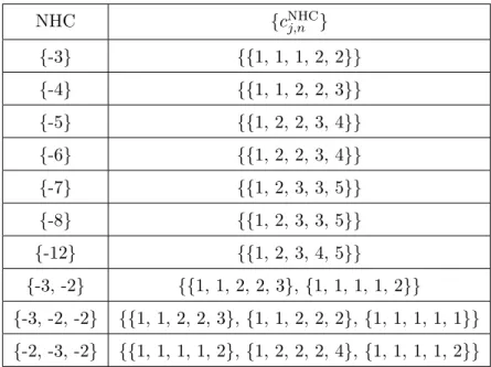
to a set of vanishing orders cj,n associated with each non-Higgsable cluster, which we list
in table5. These are the minimal values cj,n = cNHCj,n that satisfy the inequalities (2.26) for
each value of n ∈ {1, 2, 3, 4, 6}. In doing a Tate tuning, we impose the additional condition that over certain curves Cj, the vanishing order is at least some specified value that is
higher than the minimum imposed by the NHCs, cj,n ≥ ctunedj,n ≥ cNHCj,n . We can then use
the Zariski decomposition to determine the minimum values of the cj,n compatible with
this lower bound that also satisfy the inequalities (2.26).
More concretely, to determine the unique minimum set of values cj,n that satisfy the
inequalities (2.26), we proceed iteratively, following an algorithm described in appendix A of [8]. For each n, we begin with an initial assignment of vanishing orders
c(0)j,n= ctunedj,n (2.27) when we are imposing a given tuning. When we are computing the minimal values from NHC’s without tuning we simply use the minimal order of vanishing from the Zariski
JHEP02(2019)087
decomposition on each isolated curve of self-intersection mj = Mjj,
c(0)j,n = ln(2+m j) mj m , mj ≤ −3, 0, mj > −3 . (2.28) We can then use the inequalities (2.26) to determine the minimal correction that is needed to each vanishing order (label n dropped for clarity of the notation),
∆c(1)j = Max 0, & vj−PiMji (c(0)i ) mj '! . (2.29)
The second corrections are obtained similarly, replacing c(0) on the r.h.s. with c(1)= c(0)+ ∆c(1)j . We continue to repeat this procedure until the corrections in the f -th step all become zero, ∆c(f )j = 0 for all j. The final solutions {cj} are obtained iteratively this way
by adding the non-negative correction values {∆c(k)j }: cj = c(0)j + ∆c (1) j + ∆c (2) j + · · · + 0, where ∆c(l+1)j = Max 0, & vj−PiMji(c(0)i + Pl k=1∆c (k) i ) mj '! . (2.30) At each step this algorithm clearly increases the orders of vanishing in a minimal way, so when the algorithm terminates the solution is clearly a minimal solution of the inequali-ties (2.26). Note that in some cases, the algorithm leads to a runaway behavior when there is no acceptable solution without (4, 6) loci. When this occurs, or when one of the factors of the gauge algebra exceeds that desired by the tuning, we terminate the algorithm and do not consider this tuning as a viable possibility.
As an example, consider the set of curves {Cj} to be the NHC {−3, −2}, so Mji =
{{−3, 1}, {1, −2}}, and
{{v1, v2}|n = 1, 2, 3, 4, 6} = {{−1, 0}, {−2, 0}, {−3, 0}, {−4, 0}, {−6, 0}},
{{c(0)1,n, c(0)2,n}|n} = {{1, 0}, {1, 0}, {1, 0}, {2, 0}, {2, 0}}.
Then the vanishing orders calculated from (2.30) are {c1,n} = {1, 1, 2, 2, 3} and {c2,n} =
{1, 1, 1, 1, 2}, as shown in table5.
Note that a tuning beyond that shown in table 5 does not necessarily increase the gauge group on any of the curves. In particular, for some gauge groups there are multiple possible Tate tunings. Both for the generic gauge group associated with the generic elliptic fibration over a given base and for constructions with gauge groups that are enhanced through a Tate tuning, this means that there may be distinct Tate tunings with the same physical properties. As we will see later, these distinct Tate tunings can correspond through distinct polytopes to different Calabi-Yau threefold constructions. Note also that for the toric bases we are studying here, an essentially equivalent analysis could be carried out by explicitly working with the various monomials in the sections an, which in the toric context
are simply points in a dual lattice, as we discuss in the next section. We use the Zariski procedure because it is more efficient and more general; the results of this analysis should, however, match an explicit toric computation in each case.
JHEP02(2019)087
NHC {cNHC j,n } {-3} {{1, 1, 1, 2, 2}} {-4} {{1, 1, 2, 2, 3}} {-5} {{1, 2, 2, 3, 4}} {-6} {{1, 2, 2, 3, 4}} {-7} {{1, 2, 3, 3, 5}} {-8} {{1, 2, 3, 3, 5}} {-12} {{1, 2, 3, 4, 5}} {-3, -2} {{1, 1, 2, 2, 3}, {1, 1, 1, 1, 2}} {-3, -2, -2} {{1, 1, 2, 2, 3}, {1, 1, 2, 2, 2}, {1, 1, 1, 1, 1}} {-2, -3, -2} {{1, 1, 1, 1, 2}, {1, 2, 2, 2, 4}, {1, 1, 1, 1, 2}} Table 5. The minimal vanishing orders of sections a1,2,3,4,6 over NHCs.2.6 Matter content from anomaly constraints in F-theory
Six-dimensional N = (1, 0) supergravity theories potentially suffer from gravitational, gauge, and mixed gauge-gravitational anomalies. We focus here primarily on nonabelian gauge anomalies, though similar considerations hold for abelian gauge factors. On the one hand, the anomaly information can be encoded in an 8-form I8, which is built from the
2-forms characterizing the non-abelian field strength F and the Riemann tensor R, and which has coefficients that can be computed in terms of T, V, H, and the explicit numbers of chiral matter fields in different representations. On the other hand, the anomalies can be cancelled through a generalized Green-Schwarz term if I8factorizes for some constant
coef-ficients aα, bβ
i in the vector space R1,T associated with self-dual and anti self-dual two-forms
Bµν in the gravity and tensor multiplets,
I8= 1 2ΩαβX α 4X β 4, (2.31) where X4α = 1 2a αtrR2+X i bαi 2 λi trFi2. (2.32)
Here Ωαβ is a signature (1, T ) inner product on the vector space, and λi are
normaliza-tion constants for the non-abelian gauge group factors Gi. Then, using the notation and
JHEP02(2019)087
coefficients of each term from the two polynomials
R4 : H − V = 273 − 29T, (2.33) F4 : 0 = BiAdj−X R xiRBRi , (2.34) (R2)2 : a · a = 9 − T, (2.35) F2R2 : a · bi = 1 6λi A i Adj− X R xiRAiR ! , (2.36) (F2)2 : bi· bi = 1 3λ 2 i X R xiRCRi − CAdji ! , (2.37) Fi2Fj2 : bi· bj = 2 X R,S xijRSAiRAjS, i 6= j, (2.38)
where AR, BR, CR are group theory coefficients5 defined by
trRF2 = ARtrfund.F2, (2.39)
trRF4 = BRtrfund.F4+ CR(trfund.F2)2, (2.40)
xiR is the number of matter fields6 in the representation R of the non-abelian factor Gi,
and xijRS is the number of matter fields in the (R, S)-representation of Gi⊗ Gj.
For 6D theories coming from an F-theory compactification, the vectors a, biare related
to homology classes in the base B2 through the relations
a ↔ KB, (2.41)
bi ↔ Ci, (2.42)
where, again, KB is the canonical class of B2, and Ci ∈ H2(B2, Z) are irreducible curves in
the base supporting the singular fibers associated with the non-abelian gauge group factors Gi. With this identification, the Dirac inner products between vectors in R1,T are related
to intersection products between divisors in the base.
In principle, the matter content of a 6D theory can be determined by a careful analysis of the codimension two singularities in the geometry. In many situations, however, the generic matter content of a low-energy theory is uniquely determined by the gauge group content and anomaly cancellation simply from the values of the vectors a, bi. For example, a theory with an SU(N ) gauge factor associated with a vector b generically has g adjoint matter fields, (8−N )n+16(1−g) fundamental matter fields, and (n+2−2g) two-index anti-symmetric matter fields, where n = b·b and g = 1+(a·b+n)/2 (see e.g. [13]); this simplifies
5
A summary of AR, BR, CR in different representations and λi for different non-abelian gauge groups
can be found in appendix B in [13].
6For each representation the matter content contains one complex scalar field and a corresponding field
in the conjugate representation. For special representations like the 2 of SU(2), the representation is
pseudoreal, so that the conjugate need not be included; such a field is generally referred to as a “half-hypermultiplet”.
JHEP02(2019)087
in the g = 0 case of primary interest to us here to a spectrum of n+2 two-index antisymmet-ric matter fields and 16 + (8 − N )n fundamental fields. For most of the theories we consider here the matter content follows uniquely in this way from the values of a, bi. In some situations, however, more exotic matter representations can arise; we encounter some cases of this later in this paper, such as the three-index antisymmetric representation of SU(6). In general, the anomaly constraints on 6D theories provide a powerful set of consistency conditions that we use in many places in this paper to analyze and check various models that arise through tunings; in particular, using the anomaly conditions to determine the matter spectrum gives a direct and simple way in many cases to compute the Hodge numbers of the associated elliptic Calabi-Yau manifold that can be matched to the Hodge numbers of a toric hypersurface construction.
2.7 Global symmetry constraints in F-theory
In many cases, the anomaly cancellation conditions impose constraints not only on the matter content of the theory but also on what gauge groups may be combined on intersect-ing curves, correspondintersect-ing to vectors biwith non-vanishing inner products in the low-energy theory. For example, two gauge factors of g2 or larger in the Kodaira classification cannot
be associated with vectors b, b0 having b · b0 > 0; in the low-energy supergravity theory this is ruled out by the anomaly conditions while in the F-theory picture this would correspond to a configuration with a codimension two (4, 6) point at the intersection between the corresponding curves. In addition to these types of constraints, another set of constraints on what combination of gauge groups can be tuned on specific negative self-intersection curves in a base B2can be derived from the low-energy theory by considering the maximum
global symmetry of an SCFT that arises by shrinking a curve C of self-intersection n < 0 that supports a given gauge factor Gi [47]. While in most cases these global symmetry
conditions simply match with the expectation from anomaly cancellation, in some circum-stances the global symmetry condition imposes stronger constraints. For example the “E8
rule” [48] states that the maximal global symmetry on a −1 curve that does not carry a nontrivial gauge algebra is e8; i.e., the direct sum of the gauge algebras carried by the
curves intersecting the −1 curve should be a subalgebra of e8. While the global symmetry
constraints are completely consistent with F-theory geometry, they may not be a complete and sufficient set of constraints; for example a similar constraint appears to hold in F-theory for the algebras on a set of curves intersecting a 0 curve [13], though the low-energy explanation for this is not understood in terms of global constraints from SCFT’s.
The maximal global symmetry groups realized in 6D F-theory for each possible algebra on a curve of self-intersection m ≤ −1 are worked out in [47]. We use their results in our algorithm to constrain possible gauge algebra tunings. More explicitly, given a gauge algebra on a curve, the maximal global symmetry on the curve is determined, so the direct sum of the algebras on the curves intersecting it should be a subalgebra of the maximal global symmetry algebra. For instance, consider a linear chain of three curves {C1, C2, C3}
carrying gauge algebras {g1, g2, g3}. These can be either minimal or enhanced algebras,
but they have to satisfy g3⊕ g1 ⊂ g(glob)2 , where g(glob)2 is the maximal global symmetry
JHEP02(2019)087
for us to constrain the possible tunings on a curve when the gauge symmetries on its neighboring curves are known, making our search over possible tunings more efficient. This is also convenient sometimes for us to determine the gauge algebras that have monodromy conditions without having to figure out the monodromy directly; the trick to doing this is described in section 4.6. We also include the “E8 rule” in our algorithm in section5.1,
corresponding to the case where m = −1 and g2 is trivial.
2.8 Base surfaces for 6D F-theory models
There is a finite set of complex base surfaces that support elliptic Calabi-Yau threefolds. It was shown by Grassi [49] that all such bases can be realized by blowing up a finite set of points on the minimal bases P2, Fm with 0 ≤ m ≤ 12, and the Enriques surface.
This leads to a systematic constructive approach to classifying the set of allowed F-theory bases. The structure of non-Higgsable clusters limits the configurations of negative self-intersection curves that can arise on any given base, so we can in principle construct all allowed bases by blowing up points in all possible ways and truncating the set of possibilities when a disallowed configuration such as a curve of self-intersection −13 or below arises. This was used in [9] to classify the full set of toric bases B2 that can support elliptic
Calabi-Yau threefolds (toric geometry is described in more detail in the following section). While further progress has been made [10,11] in classifying non-toric bases, we focus here primarily on toric base surfaces, as these are the primary bases that arise in the toric hypersurface construction of Calabi-Yau threefolds. Note, however, that as we discuss later in the paper, particularly in e.g. section 4.7, section 6.1.3, there are cases in the Kreuzer-Skarke database where a toric polytope corresponds to an elliptic fibration over a non-toric base. The primary context in which this distinction is relevant involves curves of self-intersection −9, −10, and −11. As discussed in [8], the Weierstrass model over such curves automatically has 1, 2, or 3 points on the curve where f, g vanish to degrees (4, 6). Such points on the base can be blown up for a smooth Calabi-Yau resolution, so that the actual base supporting the elliptic fibration is generally a non-toric complex surface.7 In the simplest cases, such as F11 and F10, the blown up base still has a toric description; in
other simple cases, such as F9, the resulting surface is a “semi-toric” surface admitting only
a single C∗action [10], but on surfaces with, for example, multiple curves of self-intersection −9, −10, −11, the blow-up of all (4, 6) points in the base gives generally a non-toric base that is neither toric nor admits a single C∗ action. Despite this complication, this blow-up and resolution process is automatically handled in a natural way in the framework of the toric hypersurface construction, so that (non-flat) elliptic fibrations over bases with these types of curves arise naturally in the Kreuzer-Skarke database. Thus, we include toric bases with curves of self-intersection −9, −10, −11 in the set of bases we consider for Tate/Weierstrass constructions. The complete set of such bases was enumerated in [9], where it was shown that there are 61,539 toric bases that support elliptic CY3’s. Generic elliptic Calabi-Yau threefolds over these bases give rise to a range of Hodge number pairs
7More precisely, as described in [31] and section2.2, and discussed in more detail in section 4.7, the
original base supports an elliptic fibration that is “non-flat,” meaning that the fiber becomes two dimensional at some points, while the elliptic fibration over the blown up base is a flat elliptic fibration.
JHEP02(2019)087
that fill out the range of known Calabi-Yau Hodge numbers, in a “shield” shape with peaks at (11, 491), (251, 251), and (491, 11) [39]. As we see in section6, in some cases the base needed for a tuned Weierstrass model to match a toric hypersurface construction is even more exotic than those arising from blowing up points on curves of self-intersection −9, −10, −11. In these more complicated cases as well, however, the general story is the same. The polytope construction gives rise to a non-flat elliptic fibration with codimension two (4, 6) points on the toric base. Blowing these curves up gives rise to another, generically non-toric, base with multiple additional curves. After these blow-ups, there is a tuned Weierstrass model giving a (flat) elliptic fibration over the new base. While the toric base is what arises most clearly from the polytope construction, the structure of the blown up base admitting the flat elliptic fibration is relevant when considering F-theory models and anomaly cancellation.
In section 4 we consider Tate tunings over the toric bases and compare to the toric hypersurface construction of elliptic Calabi-Yau threefolds, which we now describe in more detail.
3 Elliptic fibrations in the toric reflexive polytope construction
3.1 Brief review of toric varieties
Following [50, 51], we review some basic features of toric geometry. An n-dimensional toric variety XΣ can be constructed by defining the fan of the toric variety. A fan Σ is a
collection of cones8 in NR= N ⊗ R, each with the apex at the origin, and where N is a rank n lattice, satisfying the conditions that
• Each face of a cone in Σ is also a cone in Σ.
• The intersection of two cones in Σ is a face of each.
Then XΣ can be described by the homogeneous coordinates zi corresponding to the
one-dimensional cones vi (also called rays) of Σ; XΣ may be constructed as the quotient of an
open subset in Ck (k is the number of rays), by a group G, XΣ = C
k− Z(Σ)
G , (3.1)
where
• Z(Σ) ⊂ Ck is the union of the zero sets of the polynomial sets S = {z
i} associated
with the sets of rays {vi} that do not span a cone of Σ.
• G ⊂ (C∗)k is the kernel of the map
φ : (C∗)k→ (C∗)n, (z1, . . . , zk) 7→ k Y j=1 zvj,1 j , . . . , k Y j=1 zvj,n j ,
where vj,l specifies the lth component of the ray vj in the coordinate representation
in Cn.
8More rigorously, these are strongly convex cones, which are generated by a finite number of vectors in
JHEP02(2019)087
Toric divisors Di are given by the sets Di ≡ {zi = 0} associated to all the rays vi. The
anti-canonical class −K of a toric variety is given by the sum of toric divisors − K =X
i
Di. (3.2)
Smooth two-dimensional toric varieties are particularly simple. The irreducible effective toric divisors are rational curves with one intersecting another forming a closed linear chain. This is easily seen from the 2D toric fan description, where each ray of the 2D fan corresponds to an irreducible effective toric divisor. The intersection products are also easy to read off from the fan diagram, where (including divisors cyclically by setting Dk+1≡ D1, etc.)
Di· Di+1= 1, (3.3)
and the self-intersection of each curve is
Di· Di = mi, (3.4)
where mi is such that
− mivi = vi−1+ vi+1, (3.5)
and zero otherwise. We will generally denote the data defining a smooth 2D toric base by the sequence of self-intersection numbers. (The 2D fan can be recovered given the intersections, up to lattice automorphisms.)
In the context of this paper, toric varieties play two distinct but related roles. On the one hand, we can use toric geometry to describe many of the bases that support elliptically fibered Calabi-Yau threefolds. On the other hand, toric geometry can be used to describe ambient fourfolds in which CY threefolds can be embedded as hypersurfaces, as we describe in the next section.
3.2 Batyrev’s construction of Calabi-Yau manifolds from reflexive polytopes Given a lattice polytope, which is the convex hull of a finite set of lattice points (in particular, the vertices are lattice points), we may define a face fan by taking rays to be the vertices of the lattice polytope, and the top-dimensional (n-dimensional) cones to correspond to the facets of the polytope. By including more lattice points in addition to vertices of the polytope as rays, and thus subdividing (“triangulating”) the facets of the polytope into multiple smaller top-dimensional cones, we can refine the fan to impose further properties such as simpliciality or smoothness.9 In this way, a lattice polytope can be associated with a toric variety. In general, a given lattice polytope can lead to many different varieties, depending upon the refinement of the face fan. Even for a given set of additional rays added, there can be many different triangulations of the fan.
9A fan is simplicial if all its cones are simplicial. A cone is simplicial if its generators are linearly
independent over R. A fan is smooth if the fan is simplicial and for each top-dimensional cone its generators generate the lattice N .
JHEP02(2019)087
We will be interested in particular in the fans from reflexive polytopes, which are defined as follows. Let N be a rank n lattice, NR≡ N ⊗ R. A lattice polytope ∇ ⊂ N containing the origin is reflexive if its dual polytope is also a lattice polytope. The dual of a polytope ∇ in N is defined to be
∇∗ = {u ∈ MR= M ⊗ R : hu, vi ≥ −1, ∀v ∈ ∇}, (3.6) where M = N∗= Hom(N, Z) is the dual lattice. If ∇ is reflexive, its dual polytope ∆ = ∇∗ is also reflexive as (∇∗)∗ = ∇. We call the pair of reflexive polytopes a mirror pair. Both of them contain the origin as the only interior lattice point. Calabi-Yau manifolds in Batyrev’s construction [52] are built out of reflexive polytopes. Given a mirror pair ∇ ⊂ N and ∆ ⊂ M , the (possibly refined) face fan of ∇ describes a toric ambient variety, in which a Calabi-Yau hypersurface is embedded using the anti-canonical class of the ambient toric variety, so that the hypersurface itself has trivial canonical class. Explicitly, a section of the anti-canonical bundle is given by
p =
# lattice points in ∆
X
i
cimi, (3.7)
where ci are generic coefficients taking values in C and each monomial mi is given by an
associated lattice point wi in ∆
mi=
Y
j
zhwi,vji+1
j , (3.8)
where zj is the homogeneous coordinate associated with the ray vj in the fan associated
to ∇. The well-definedness of each mi in terms of the homogeneous coordinates zj is
guaranteed by the linear equivalence relations among the divisors associated to vj’s, and
holomorphicity in the zjs by the reflexivity of ∇. We can check that equation (3.7) indeed
defines a section of the anti-canonical class, so that a CY hypersurface is cut out by p = 0. We can determine the class by looking at any one of the monomials; we pick the origin since we know it is always an interior point. Its associated monomial by equation (3.8) is simply the product of all homogeneous coordinates associated to all toric divisorsQ# rays
j=1 zj,
which immediately we see by equation (3.2) is a section in the anti-canonical class. For the smoothness of the Calabi-Yau, as mentioned previously, there exists a refinement10 of the face fan of ∇ such that the fan is simplicial so the ambient toric variety will have at most orbifold singularities. In the case of n ≤ 4, with the anti-canonical embedding, a hypersurface will generically avoid these singularities and therefore is generically smooth.
M. Kreuzer and H. Skarke have classified all 473,800,776 four-dimensional reflexive polytopes for the Batyrev Calabi-Yau construction [4,53]. A pair of reflexive polytopes in the KS database are described in the format:
M:# lattice points, # vertices (of ∆) N:# lattice points, # vertices (of ∇) H: h1,1, h2,1.
10
Appropriate subdivisions of the face fan of the toric ambient variety by additional lattice points in the facets of the polytope give the resolved description of the embedded Calabi-Yau, where extra coordinates in
equation (3.8) define the exceptional divisors in the resolution of the ambient space. The added lattice points
that do not lie in the interior of the facets also correspond to exceptional divisors in the resolution of the Calabi-Yau. (Generic hypersurface CYs do not meet the divisors that correspond to interior points of facets.)
JHEP02(2019)087
We will refer to ∇ as the (fa)N polytope and ∆ as the M(onomial) polytope to remind ourselves that ∇ gives the fan of the ambient toric variety for the CY anti-canonical embed-ding and ∆ determines the monomials of the anti-canonical hypersurface. In many cases, it is sufficient to specify polytopes with the information given in the format above, but sometimes there can be distinct polytopes with identical information of this type, in which case we will either give further the vertices of the N polytope to specify the polytope more precisely, or indicate its numerical order as it appears among those with identical data in the KS database website (http://hep.itp.tuwien.ac.at/∼kreuzer/CY/) with a superscript, e.g., M:165 11 N:18 9 H:9,129[1] or M:165 11 N:18 9 H:9,129[2].
Note that conversely, we can start from ∆ and associate it with the polytope that defines the fan of the ambient space, and calculate monomials associated with lattice points in ∇. Then the hypersurface CY is mirror to the previous one. The Hodge numbers of mirror pairs are related by hp,q(CY∇) = hd−p,q(CY∆), where d = n − 1 is the complex
dimension of the CY; in particular, we will look at 4 dimensional reflexive polytopes for CY threefolds, where the only non-trivial Hodge numbers are h1,1 and h2,1, and mirror CY hypersurfaces have exchanged values for h1,1 and h2,1. As ∇ and ∆ are a pair of 4D reflexive polytopes, there is a one-to-one correspondence between l-dimensional faces θ of ∆ and (4 − l)-dimensional faces ˜θ of ∇ related by the dual operation
θ∗= {y ∈ ∇, hy, pti = −1| for all pt that are vertices of θ} . (3.9) For the CY associated with ∇, the Hodge numbers are given by
h2,1= pts(∆) − X θ∈F∆ 3 int(θ) + X θ∈F∆ 2 int(θ)int(θ∗) − 5, (3.10) h1,1= pts(∇) − X ˜ θ∈F∇ 3 int(˜θ) + X ˜ θ∈F∇ 2 int(˜θ)int(˜θ∗) − 5, (3.11)
where θ are faces of ∆, ˜θ are faces of ∇, Fl∇/∆ denotes the set of l-dimensional faces of ∇ or ∆ (l < n), and pts(∇/∆) := number of lattice points of ∇ or ∆, int(θ/˜θ) := number of lattice points interior to θ or ˜θ. The correspondence (3.9) makes the duality between the Hodge number formulae manifest. Note that the Hodge numbers depend only on the polytope and not on the detailed refinement of the fan.
3.3 Fibered polytopes in the KS database
For the purpose of studying (often singular) elliptically fibered Calabi-Yau threefolds that arise in the KS database, we will be interested in 4D reflexive fibered polytopes [31,54–56]. A fibered polytope ∇ is a polytope in the N lattice that contains a lower-dimensional subpolytope, ∇2 ⊂ N2 = Z2, which passes through the origin. We are interested in the
case where ∇2 is itself a reflexive 2D polytope, containing the origin as an interior point.
Such a fibered polytope ∇ admits a projection map π : ∇ → NB such that π−1(0) = ∇2,
and NB= Z2 is the quotient of the original lattice N by the projection. We can construct
a set of rays vi(B) in NB that are the primitive rays with the property that an integer
JHEP02(2019)087
cannot be described as an integer multiple v = nw of another ray w ∈ N , with n > 1.) We define the base B2 to be the 2D toric variety given by the 2D fan ΣB with v(B)i taken to
be the 1D cones; the 2D cones are uniquely defined for a 2D variety. Note that in higher dimensions, the base of the fibration is not uniquely defined as a toric variety since the cone structure of the base may not be unique.
In the toric geometry language, a fan morphism is a projection π : Σ → ΣB with
the property that for any cone in Σ the image is contained in a cone of ΣB. Such a fan
morphism can be translated to a map between toric varieties π : XΣ → B2. Such a map
is a toric morphism, which is an equivariant map with respect to the torus action on the toric varieties that maps the maximal torus in XΣ to the maximal torus in B2. As far as
the authors are aware, it is not known whether in general every fibered polytope admits a triangulation leading to a compatible fan morphism and toric morphism. Note, however, that the elliptic fiber structure of the polytope does not depend upon the existence of a triangulation with respect to which there is a fan morphism π : Σ∇ → ΣB. Thus, to
recognize an elliptic Calabi-Yau threefold in the KS database, it is only necessary to find a reflexive subpolytope ∇2 ⊂ ∇. The Calabi-Yau manifold defined by an anti-canonical
hypersurface in XΣ through the Batyrev construction with reflexive polytopes will then be
an elliptically fibered Calabi-Yau threefold over the base B2 [55]. A primary goal of this
paper is to relate reflexive polytopes in the Kreuzer-Skarke database that have this form to elliptic fibrations of tuned Weierstrass models as described in section 2.
There are in total 16 2D reflexive polytopes, which give slightly different realizations of an elliptic curve when an anti-canonical hypersurface is taken [23,31,57]. The hypersurface equations p = 0, with p given in (3.7), of all 16 types of fibered polytopes can be brought into the Weierstrass form (2.8) by the methods described in appendix A in [31]; this gives an equivalent description of the same Calabi-Yau as long as the fibration has a global section. The Kreuzer-Skarke database of reflexive polytopes and associated Calabi-Yau hypersurface constructions contains a wide range of polytopes that include fibered polytopes with many different examples of the 16 fiber types.
For a given base B2 and a given fiber type, there can be a variety of different polytopes
corresponding to configurations with different “twists” of the fibration, associated with dif-ferent embeddings of the rays videfining the base B2 with respect to the fiber subpolytope
∇2. For example, the Hirzebruch surfaces Fm are each associated with fibered polytopes
with fiber and base P1, distinguished by the different twists of the fibration. For a fibered polytope ∇ with a reflexive subpolytope ∇2, the dual ∆ admits a projection to ∆2 = (∇2)∗.
One of the findings of this paper is that the bulk of KS models with large Hodge numbers appear to have a description in the form of a standard P2,3,1-fibered type, with a specific form for the twist of the fiber over the base surface B2; these models can be
con-nected directly to the Tate form for elliptic fibrations, and in fact can be constructed from that point of view directly. On the one hand, we describe the structure of this type of stan-dard polytope in section3.4, with the result that the anti-canonical hypersurface equations from (suitably refined) standard P2,3,1-fibered polytopes are in the form of equation (2.14). On the other hand, we describe the direct construction of polytopes by carrying out Tate tunings on the effective curves in the toric bases in section 4, and develop an algorithm
JHEP02(2019)087
(a) The toric fan for P2,3,1. The convex hull
of P2,3,1 plays the role of the reflexive
sub-polytope ∇2 for standard P2,3,1-fibered
poly-topes ∇ in the N lattice. The rays vx, vy, vz
are associated with the homogeneous coordi-nates x, y, z, respectively, in the hypersurface equation.
(b) The dual polytope ∆2 to ∇2 in the M2
lattice. Projection onto the M2plane projects
the lattice points in ∆ into seven lattice points in ∆2. These lattice points correspond to the
five sections a1,2,3,4,6 in the Tate form of the
Weierstrass model, indicated in the figure by xyz, x2z2, yz3, xz4, z6, respectively, and to the coefficients of the remaining two terms x3, y2 in the hypersurface equation.
Figure 1. The reflexive polytope pair for the P2,3,1 ambient toric fiber.
in section 5 to systematically classify models of this type that give polytopes and elliptic Calabi-Yau threefolds with large Hodge numbers; these models are all expected to have a corresponding standard P2,3,1-fibered polytope, and we compare the two constructions in the remainder of section6. For a given base B2 there are generally many distinct polytopes
that have the standard P2,3,1-fibered structure; as we describe in the following section, these correspond to different Tate tunings over the same base.
3.4 Standard P2,3,1-fibered polytopes and corresponding Tate models
The fiber polytope ∇2 that provides a natural correspondence with the Tate form
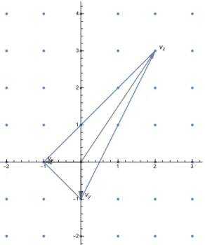
mod-els (2.14) is associated with the toric fan giving the weighted projective space P2,3,1; this is a toric variety given by the rays vx = (−1, 0), vy = (0, −1), vz = (2, 3) (see figure 1a).
Given a P2,3,1-fibered polytope ∇ over a toric base B2, where the fiber is defined by three
rays satisfying 2vx+ 3vy+ vz = 0, we can always perform a SL(2, Z) transformation to put
the rays in the fiber into the coordinates