Computational phase imaging based on intensity transport

Computational Phase Imaging based

on Intensity Transport

by

Laura A. Waller

B.S., Massachusetts Institute of Technology (2004)

M.Eng., Massachusetts Institute of Technology (2005)

MASSACHUSETTS INSTITUTE OF TECHNOLOGY

JUL 12 2010

LIBRARIES

ARCHIVES

Submitted to the Department of

Electrical Engineering and Computer Science

in partial fulfillment of the requirements for the degree of

Doctor of Philosophy in Electrical Engineering and Computer Science

at the

MASSACHUSETTS INSTITUTE OF TECHNOLOGY

June 2010

©

Massachusetts Institute of Technology 2010.

Author ...

...

All rights reserved.

Department of

Electrical Engineering and Computer Science

'-

h\

f'\

May 14, 2010

Certified by....

George Barbastathis

Associate Professor of Mechanical Engineering

Thesis Supervisor

Accepted by...

-Terry P.

Orlando

Chairman, Department Committee on Graduate Theses

Computational Phase Imaging based

on Intensity Transport

by

Laura A. Waller

Submitted to the Department of Electrical Engineering and Computer Science

on May 14, 2010, in partial fulfillment of the requirements for the degree of

Doctor of Philosophy in Electrical Engineering and Computer Science

Abstract

Light is a wave, having both an amplitude and a phase. However, optical frequencies are too high to allow direct detection of phase; thus, our eyes and cameras see only real values - intensity. Phase carries important information about a wavefront and is often used for visualization of biological samples, density distributions and surface profiles. This thesis develops new methods for imaging phase and amplitude from multi-dimensional intensity measurements. Tomographic phase imaging of diffusion distributions is described for the application of water content measurement in an operating fuel cell. Only two projection angles are used to detect and localize large changes in membrane humidity. Next, several extensions of the Transport of Intensity technique are presented. Higher order axial derivatives are suggested as a method for correcting nonlinearity, thus improving range and accuracy. To deal with noisy images, complex Kalman filtering theory is proposed as a versatile tool for complex-field estimation. These two methods use many defocused images to recover phase and amplitude. The next technique presented is a single-shot quantitative phase imag-ing method which uses chromatic aberration as the contrast mechanism. Finally, a novel single-shot complex-field technique is presented in the context of a Volume Holographic Microscopy (VHM). All of these techniques are in the realm of compu-tational imaging, whereby the imaging system and post-processing are designed in parallel.

Thesis reader: James Fujimoto, Professor of Electrical Engineering, MIT Thesis reader: Cardinal Warde, Professor of Electrical Engineering, MIT

Thesis reader: Colin J. R. Sheppard, Professor, Head of Division of Bioengineering, National University of Singapore

Thesis Supervisor: George Barbastathis

Acknowledgments

Having been at MIT for - 1/3 of my life, I will always appreciate having spent the

formative years of my education at such a unique and wonderful institution. It is the intelligent, passionate people who make this place unlike any other, and I can only name a few here. First and foremost, I want to thank my advisor, Prof. George Barbastathis, for his guidance, knowledge and mentorship, and for creating a truly academic environment for learning and research. I thank my thesis readers, Prof. James Fujimoto and Prof. Cardinal Warde, for insightful suggestions, and especially Prof. Colin Sheppard, who has always welcomed me into his lab in Singapore to discuss ideas and borrow equipment.

I have learned something from all of my colleagues in the 3D Optical Systems group, and I thank in particular Pepe Dominguez-Caballero, Nick Loomis, Se Baek Oh, Lei Tian and Hanhong Gao for all the whiteboard discussions, and Satoshi Taka-hashi, Chi Chang, Se Young Yang and Nader Shaar for their 'nano' help. I also thank everyone at my second research home in Singapore -members of CENSAM, BIOSYM and the NUS Bioimaging Lab, especially Shan Shan Kou, my collaborator and friend. Specific recognition goes to Jungik Kim and Prof. Yang Shao-Horn for fuel cell expertise, Mankei Tsang for the idea and help with Kalman filters, Yuan Luo for use of and help with the VHM system, the MIT Kamm lab and Yongjin Sung for cell samples, Boston Micromachines and Prof. Bifano of BU for use of the deformable mirror array. Furthermore, none of this work would have been possible without funding from the Dupont-MIT Alliance (DMA) and the Singapore-MIT Alliance for Research and Technology (SMART).

Finally, I thank my friends and family for making life fun, particularly Sameera Ponda and my awesome boyfriend, Robin Riedel, who is my best friend and greatest advocate. My parents, Eva and Ted, and my sister Kathleen were collaborators in my first backyard optics experiments and taught me by example the importance of education. After 22 years of school, I am no longer a student, but I will never stop learning.

Contents

1 Introduction 21

1.1 Phase contrast . . . . 22

1.2 Interferometric phase imaging techniques . . . . 23

1.2.1 Phase-shifting interferometry . . . . 23

1.2.2 Digital holography . . . . 24

1.2.3 Differential interference contrast microscopy... . . . .. 26

1.3 Non-interferometric phase imaging techniques . . . . 27

1.3.1 Shack-Hartmann sensors . . . . 27 1.3.2 Iterative techniques . . . . 27 1.3.3 Direct methods . . . . 29 1.3.4 Transport of Intensity . . . . 29 1.3.5 Estimation theory . . . . 30 1.4 Computational imaging . . . . 30 1.5 O utline of thesis . . . . 31 2 Complex-field tomography 33 2.1 Tom ography . . . . 33

2.1.1 The projection-slice theorem . . . . 34

2.1.2 Filtered back-projection . . . . 35

2.2 Phase tomography . . . . 36

2.2.1 Phase-shifting complex-field tomography.. . . . . . . . . . 37

2.2.2 Experimental results . . . . 38

2.3 Sparse-angle tomography of diffusion processes . . . . 42

2.3.1 Projections of diffusion distributions... . . . .. 43

3 Two angle interferometric phase tomography of fuel cell membranes 45 3.1 Introduction... . . . . . . . . 45

3.2 O ptical system . . . . 48

3.3 Sampling diffusion-driven distributions... ... . .. 50

3.4 Temporal phase unwrapping . . . ... . . . . 53

3.5 Two angle tomography... . . . . . . .. 53

3.6 Experimental results... . . . . . . .. 54

3.7 Discussion... . . . . . . . . 57

4 Transport of Intensity imaging 59 4.1 T heory . . . . 60

4.1.1 Analogies with other fields... . . . . .. 61

4.2 Solving the TIE . . . . 62

4.2.1 Poisson solvers . . . . 63 4.2.2 Boundary conditions... . . . .. 63

4.2.3

Measuring

/az....

. . . .

. . . .

64

5 Transport of Intensity imaging with higher order derivatives 71 5.1 TIE imaging with many intensity images . ... . . . . 71

5.2 T heory . . . . 72

5.2.1 Derivation.. . . . . . . . 72

5.2.2 Technique 1: Image weights for measuring higher order derivatives 74 5.2.3 Technique 2: Polynomial fitting of higher orders . . . . 76

5.4 Experimental results . . . . 80

5.5 D iscussion . . . . 82

6 Complex-field estimation by Extended Kalman Filtering 85 6.1 Optimal phase from noisy intensity images . . . . 85

6.2 T heory . . . . 86

6.3 Implementation . . . . 90

6.3.1 Compression method 1. Fourier compression . . . . 91

6.3.2 Compression method 2. Block processing . . . . 91

6.4 Sim ulations . . . . 92

6.5 Experimental Results . . . . 96

6.6 D iscussion . . . . 96

7 Phase from chromatic aberrations 99 7.1 Introduction . . . . 99

7.2 T heory . . . . 101

7.2.1 D erivation . . . . 102

7.2.2 Resolution, accuracy and noise considerations . . . . 103

7.3 Controlling chromatic aberration . . . . 104

7.3.1 Chromatic defocus in a 4f system . . . . 105

7.3.2 Lateral chromatic aberration . . . . 106

7.3.3 Choice of color camera . . . . 107

7.3.4 Imaging with achromats . . . . 107

7.4 Experimental results . . . . 109

7.4.1 Material dispersion considerations . . . 111

7.5 Comparison with other methods . . . . 112

7.6 Real-time computations on a GPU . . . . 113

7.7 D iscussion . . . . 115

8 Quantitative phase imaging in a Volume Holographic Microscope 117 8.1 Introduction . . . . 117

8.2 _{Volume Holographic Microscopy . . . 117}

8.3 The VHM system . . . 119

8.4 TIE in the VHM... . . . . . . . 120

8.5 Experimental results ... . 121

8.6 _{D iscussion . . . 123}

9 Conclusions and future work ₁₂₅

A Derivation of Poynting vector S oc IV1

#(x,

List of Figures

1-1 Complex-field of a HeLa cell sample. (a) Amplitude transmittance shows no contrast because the cells are transparent. (b) Phase image, obtained by method of Chapter 7, reveals details of the projected density. 21 1-2 Original phase contrast image, by F. Zernike, 1932 [1]. . . . . 22 1-3 Phase-shifting interferometry of a cubic phase plate. . . . . 24 1-4 Twin image problem. (a) Amplitude reconstruction without phase

in-formation at hologram plane, (b) amplitude reconstruction with phase inform ation. . . . . 24 1-5 Two different complex fields having the same propagated intensity. . . 26 1-6 Schematic of an iterative technique, with two images in the Fresnel

domain. V) is the complex-field at the first image plane and h is the propagation kernel. . . . . 28 1-7 A plane wave passing through a phase object. Grey arrows are rays

and blue dashed lines are the associated wavefronts. . . . . 29 2-1 The Radon transform. (a) Object density map f(x, y) and (b) its

Radon transform . . . . 34 2-2 The Projection-slice theorem. . . . . 35 2-3 Filtered back-projection. (a) Sampling in the Fourier domain by

pro-jections, (b) a Hamming window (top) is pixel-wise multiplied by a Ram-Lak filter (middle) to get the Fourier domain projection filter (bottom). (c) Reconstruction using 180 projections. . . . . 36 2-4 Tomographic arrangement in a Mach-Zehnder interferometer. . . . . . 37

2-5 Sample 2D cross-sections of 3D complex-field objects immersed in index-matching fluid... _{. . . ... 39} 2-6 Left: Tomographic error due to phase-shifting. Right: Error maps for

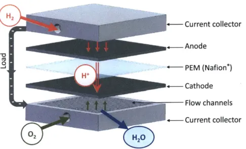
reconstruction of null object (phase in radians). Error bars indicate standard deviation. a) Type I, b) Type II, c) Type III, d) Type IV, e) Type V error. . . . . 41 3-1 Schematic of a PEM fuel cell system. . . . . 46 3-2 _{Double Mach-Zehnder interferometer configuration. Waveplates are}

used to _{adjust the relative intensities of the reference and object arms. 47}

3-3 Optical model of light in system. . . . . 48 3-4 In-plane images a) interferogram and b) amplitude only. . . . . 49 3-5 Effect of membrane edge polishing. a) Unpolished edge, b)

interfer-ogram with unpolished membrane, c) polished edge, d) interferinterfer-ogram with polished membrane. . . . . 49 3-6 Backpropagated solution using Gerchberg-Saxton-Fienup type

itera-tive method in the Fresnel domain with 50 iterations. (a) Amplitude and (b) phase. . . . . 50 3-7 Unwrapping intensity variations. (a) Intensity vs time for one pixel,

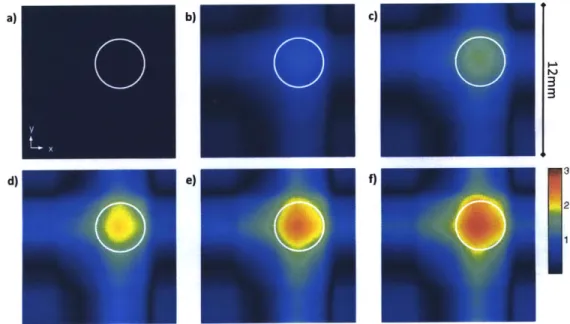
while humidifying. Circles indicate detected peaks and valleys. (b) Water content change vs time after phase unwrapping and conversion. 51 3-8 Experimental results for a test object. 2D water content

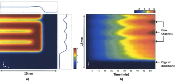
reconstruc-tions after a) 0 s, b) 160 s, c) 320 s, d) 480 s, e) 640 s, f) 800 s. The white circle indicates the location of the water drop. . . . . 55 3-9 (a) FEM simulation of water diffusing outward from flow channels in

one section of the Nafion@ membrane after 3 min. (b) Projection data over time for one angle. Three individual flow channels are resolved. . 56 3-10 Experimental results for fuel cell. 2D water content reconstructions

4-1 (a) Test phase object with non-zero boundary conditions (radians). (b) Error plot as padding is increased (number of extra pixels added to each edge). . . . . 64 4-2 Error mechanisms in TIE imaging. (a) Noise corrupted reconstruction

at small Az, (b) actual phase, (c) error in phase reconstruction for increasing Az. Error bars denote standard deviation, and FFT and Multi-grid refer to the method of Poisson solver. (d) Nonlinearity cor-rupted phase reconstruction at large Az, and (e) phase reconstruction at optimal Az. Phase color scale is 0 -7r. . . . . 65 4-3 (a) Error in reconstructions as Az is increased for increasing amounts

of added noise. Added noise increases the optimal Az value and (b) increases the error in the optimal reconstruction nonlinearly. . . . . . 66 4-4 Error plots vs. defocus distance for noisy data, where averaging two

images leads to a significant improvement in the optimal phase recon-struction . . . . . 66 4-5 (a) Error in reconstructions as Az is increased for increasing smoothing

factor (sf). The 'nonlinearity line' is lower for smoother objects and (b) error drops quickly with smoothness. . . . . 67

5-1 Higher order derivative components (bottom) of axial intensity for a propagating test object having separate amplitude and phase variations (top). Note unequal scale bars. . . . . 73 5-2 Plot of simulated nonlinearity error for two different phase objects as

Az increases, showing improvement when using 2 nd order TIE. Inset

shows in focus phase image for (a) test phase object and (b) random phase object. Phase values are radians. . . . . 77 5-3 Error plots with test object in Fig. 5-2(b) for increasing Az with a) no

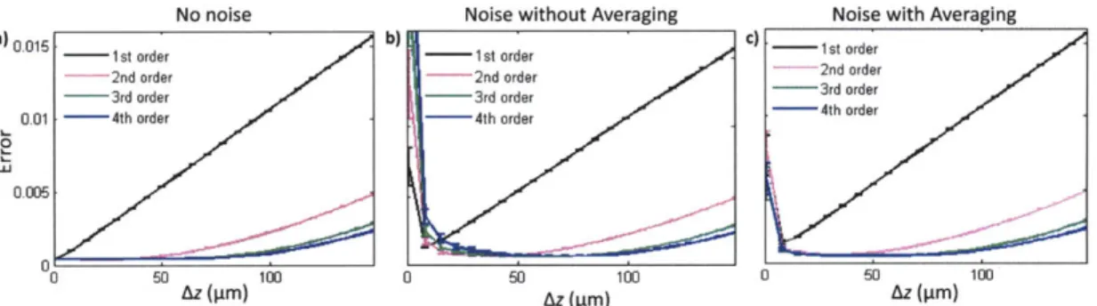
noise, b) noise (standard deviation a = 0.001) with no averaging, c) noise with averaging. Error bars denote standard deviation. . . . . . 78

5-4 (a) Simulated intensity focal stack with a pure phase object (max phase 0.36 radians at focus). (b) Axial intensity profile for a few randomly selected pixels. (c) Single pixel intensity profile with corresponding fits to 1s, 7th and 1 3th orders, having 0.0657,0.0296 and 0.0042 RMS fit

error, respectively.. . . . . . . . 79 5-5 Simulation of phase recovery improvement by fitting to higher order

polynomials. Top row: Recovered phase (radians). Bottom row: Error maps for corresponding phase retrieved. Polynomial fits are, from left to right, 1" order, 7th order, 1 3th order, and 2 0th order. . . . . 79 5-6 Actual error and RMS fit error for increasing fit orders. . . . . 80 5-7 Phase reconstructions from simulated noisy intensity images for

differ-ent phase retrieval algorithms. Color bars denote radians. . . . . 81 5-8 Experimental reconstruction of a phase object using different

recon-struction algorithms. Top row: subset of the through-focus diffracted intensity images with Az = 5pim and effective pixel size of 0.9pm. Bottom row: Traditional TIE phase reconstruction, Soto method, iter-ative method after 500 iterations, and 2 0th order TIE using technique 2 (radians). . . . . 82 5-9 Experimental reconstruction of a test phase object from multiple

in-tensity images in a brightfield microscope. Top row: Phase reconstruc-tions (radians), Bottom row: amplitude reconstrucreconstruc-tions. Left column: technique 1 (4th order), Right column: technique 2 (4'h order). .... 83

6-1 Kalman filter schematic diagram... . . . . . . . . .. . 90

6-2 Simulated results using Kalman field estimation. Left: selected images from the noisy measurements. Right: actual amplitude and phase at focus compared to the recovered amplitude and phase (radians). . . . 92

--6-3 Progress of Kalman field estimation. Row 1: Actual intensity as field propagates, Row 2: evolution of intensity estimate from Kalman filter (starts with zero initial guess), Row 3: actual phase (radians) as field propagates, Row 4: evolution of phase estimate (radians) from Kalman filter. . . . . 9 3 6-4 Error convergence for Kalman filter as images are added. . . . . 94 6-5 Axial intensity curve for a single pixel and its corresponding noisy

measurements (Poisson noise, o- = 0.999). . . . . 94 6-6 Phase retrieval comparison with other techniques. All scale bars

indi-cate radians.. . . . . 95 6-7 Simulated results using Kalman field estimation with Fourier

compres-sion. Data set uses 50 images having Az = 0.2pn and noise o = 5.5. The image is 100 x 100 pixels in size, and 18 x 18 state variables are used. Left: images from actual intensity as light propagates and the noisy measured images. Right: actual amplitude and phase at focus, compared to the recovered amplitude and phase (radians). . . . . 95 6-8 Experimental setup using laser illumination and 4f system, with

cam-era on a motion stage for obtaining multiple images in sequence. . . . 96 6-9 Experimental results using Kalman field estimation with block

pro-cessing. Left: measured images, Right: recovered amplitude and phase (radians). . . . . 97 7-1 Free-space diffraction from a phase object exhibits chromatic

disper-sion, such that the three color channels (R-red, G-green, B-blue) record different diffracted images. . . . . 101 7-2 Noise-free error simulation for varying values of wavelength and z with

a random test phase object. In the absence of noise, the error goes asymptotically to zero with decreasing defocus. . . . . 103 7-3 Validity range for accurate phase imaging. x is the characteristic object

7-4 Chromatic 4f system for controlling wavelength-dependent focus: schematic of ray trace for red, green and blue wavelengths. . . . . 105 7-5 Design of a chromatic 4f system for differential defocus of color

chan-nels. (a) Quantification of chromatic defocus for three values of f2 given fi = _{200mm with BK7 lens dispersion, (b) spot diagram at}

image showing negligible lateral chromatism. . . . 106 7-6 (a) Bayer filter color pattern, (b) spectrum of filters in standard

Bayer-filter cam era. . . . 107 7-7 Imaging with achromatic lens. (a) Focal shift plot for standard

achro-matic lens, (b) phase result using standard processing, (c) phase result using achromatic processing. . . . 108 7-8 _{Experimental setup for deformable mirror experiments. . . . 109} 7-9 _{Phase retrieval from a single color image. (a-c) Red, green and blue}

color channels, (d) captured color image of DM with 16 posts actuated. (e) Phase retrieval solution giving inverse height profile across the mirror. 110 7-10 Phase retrieval in a standard brightfield microscope. (a) Color image

of PMMA test object, (b) recovered phase map (colorbar indicates nm). (c) Color image of live HMVEC cells, (d) recovered optical path length map (normalized). (e) Color image of HeLa cells, (f) Phase map (normalized). . . . .111 7-11 Comparison with commercial profilometer data. (Left) Height map

from Zygo interferometer compared to (Middle) height map from the technique described here. Colorbar indicates height in ym. (Right) Cross-section along one actuator (influence function of DM) using both techniques . . . 113 7-12 Comparison with traditional TIE. (Left) Normalized optical path length

(OPL) from traditional TIE, (Middle) normalized OPL from our tech-nique and (Right) the difference between the two results. . . . . 113 7-13 Schematic of processing steps on the GPU. Det: detector, CPU: host

7-14 Snapshot from real-time reconstruction. Contrast was adjusted for display . . . . 115 7-15 GPU performance. (a) Computation time vs. number of pixels in

image, (b) GPU speed/camera read-in speed vs. framerate. . . . . 115 8-1 Schematic of a VHM system. The VH is located on the Fourier plane

of the 4f system, and each multiplexed grating acts as a spatial-spectral filter to simultaneously project images from different depths on a CCD camera, laterally separated. MO is microscope objective. . . . . 119 8-2 (a) Bragg circle diagram (b) Geometry analysis of a volume holographic

grating (image courtesy of Yuan Luo). . . . . 120 8-3 Phase recovery from a VHM image. (a) Image captured by the camera.

(b,c) Extracted background normalized sub-images, over and under-focused by the same amount. (d) Recovered height. . . . . 122 8-4 Comparison of phase recovery methods with an onion skin object. (a)

Phase from traditional TIE method (Az = 50pm), (b) phase from a single-shot VHM system (radians). . . . . 122

List of Tables

2.1 Types of phase-shifting error . . . . 40 4.1 Analogies to the continuity equation . . . . 62 5.1 Finding image weights for a desired order of accuracy. . . . . 76

Chapter 1

Introduction

Phase is an important component of an optical field that is not accessible directly by a traditional camera. Transparent objects, for example, do not change the am-plitude of the light passing through them, but introduce phase delays due to regions of higher optical density (refractive index). Where these phase delays can be mea-sured, previously invisible information about the shape and density of the object can be obtained (see Fig. 1-1). Optical density is related to physical density, so phase images can give distributions of pressure, temperature, humidity, or other material properties [2]. Furthermore, in reflection mode, phase carries information about the topology of a reflective object and can be used for surface profiling.

Amplitude

Figure 1-1: Complex-field of a HeLa cell sample. (a) Amplitude transmittance shows no contrast because the cells are transparent. (b) Phase image, obtained by method of Chapter 7, reveals details of the projected density.

When objects are semi-transparent, it becomes important to be able to separate phase effects from those due to absorption. Since only intensity measurements are

made, decoupling phase and amplitude generally requires two measurements for each data point. Techniques which can fully decouple phase from amplitude will be referred to as 'complex-field' imaging techniques, or 'quantitative phase imaging', since they provide a linear map of phase values.

1.1

Phase contrast

The first phase visualization techniques were not quantitative. In the early 1900s, mi-croscopists recognized that a focused image contains no phase information, whereas a slightly defocused image reveals something about the phase of the object [1]. Indeed, an in-focus imaging system has a purely real transfer function and thus no phase contrast. Defocus introduces an imaginary component, converting some phase infor-mation into intensity changes [3, 4]. However, the phase to intensity transfer function is generally nonlinear. Thus, a defocused image of a phase object is neither in-focus nor quantitative, yielding only a qualitative description of the object.

Phase contrast microscopy [5] solved the problem of providing in-focus phase con-trast, for which Frits Zernike won the Nobel prize in 1953. The method uses a phase mask to shift only the DC term, such that it interferes with higher spatial frequencies. This provides a simple, efficient method for converting phase information to intensity information (see Fig. 1-2), however, is not a quantitative technique.

a) b)

Brightfield Phase contrast

1.2

Interferometric phase imaging techniques

With the invention of the laser, coherent interference techniques for phase retrieval became accessible, allowing extremely sensitive phase measurements (up to A/100)

[6].

#(x,

I(x, y) = (x, y) + Ar e2 (1.1)

A(x, y) 2 +|A 2 + 2|A(x, y)A,| cos(#(x, y) - 0).

Again, intensity is a function of both amplitude and phase, so the technique is not quantitative.

1.2.1

Phase-shifting interferometry

Interferometry can become a complex-field technique by phase-shifting the reference beam at least twice by a known small amount (usually A/2) and using multiple images to reconstruct the phase distribution [7]. Sequential capture of the images leads to experimental complexities which will be discussed in Chapter 2. Pixellated phase-shift masks use a different method for single-shot phase imaging by phase-shifting every 4 th pixel [8, 9].

Since the measurement is related to the cosine of the phase, there will be 27r ambi-guities and an unwrapping process is required [10]. A sample interferogram is shown in Fig. 1-3 along with the recovered amplitude map and the wrapped and unwrapped quantitative phase maps. Images were obtained in a Mach-Zehnder interferometer with four phase-shifted images and the unwrapping method proposed by Ghiglia [11]. The phase object is a cubic phase plate from CDM Optics.

Interrerogram

Figure 1-3: Phase-shifting interferometry of a cubic phase plate.

1.2.2

Digital holography

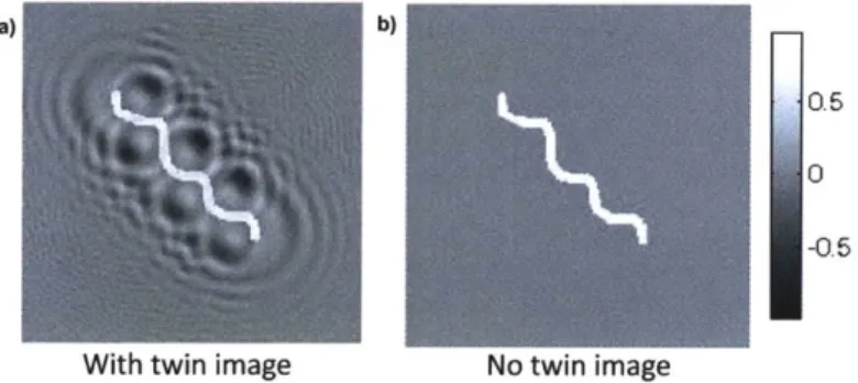
Digital holography (DH) is an interferometric method where light diffracts from an object and the intensity of that diffraction pattern is captured on a camera [12, 13, 14, 15]. Since we know exactly how light propagates, the field can be digitally back-propagated to the focal plane of the object within any linear isotropic medium (or nonlinear medium [16]). When the phase of the diffracted field at the camera is not measured, it must be assumed, leading to the 'twin-image' problem, an artifact caused by a defocused replicate of the object at twice the distance (see Fig. 1-4). Phase-shifting [17] or other phase imaging methods which capture both the amplitude and phase at the camera plane do not suffer from the twin image problem.

a) b)

0.6

0

-0.5

With twin image No twin image

Figure 1-4: Twin image problem. (a) Amplitude reconstruction without phase infor-mation at hologram plane, (b) amplitude reconstruction with phase inforinfor-mation.

One popular alternative to complex-field DH is the off-axis configuration [18, 19]. By adding a tilt to the reference beam, a spatial carrier frequency modulates the diffracted field and shifts the object and twin image spectrum to different parts of the Fourier plane, such that they can be extracted independently by selecting out the proper section of the hologram's Fourier transform. The major advantage is the capability for single-shot complex-field imaging, at the cost of a large loss in resolution, since only a small number of the total available pixels are used.

The importance of phase in propagation

Light propagation under the Fresnel approximation is a convolution of the field with the quadratic pure-phase factor given by the Fresnel kernel [20],

i27rz/A

r

h(x, y;

A

z)

=

-

exp,

(x2

(+

y2)

(1.2)

The intensity of the propagated field is:

I(x, y; Az) =

1,0(x,

9

= .71

{I(u,

v;

(1.3)

where 9 denotes convolution, T-1 denotes 2D inverse Fourier transform, u, v are the spatial frequency variables associated with x, y, TI(u, v) is the Fourier transform of the field to be propagated, A is the wavelength of illumination, z is the propagation distance, and H(u, v; Az) = F {h(x, y; Az)} is the Fourier domain Fresnel kernel.

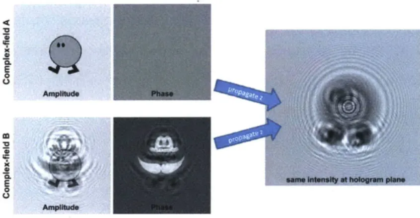
Since propagated intensity is dependent on both amplitude and phase, both are needed to back-propagate the field uniquely. As an example, Fig. 1-5 shows two different complex-fields which produce the same intensity pattern after propagation by the same distance. If one were to measure the phase of the propagated fields, they would not be the same. This emphasizes the benefits of measuring the full complex field in DH experiments.

Figure 1-5: Two different complex fields having the same propagated intensity.

1.2.3

Differential interference contrast microscopy

Differential interference contrast (DIC) [21, 22] is a popular technique for phase

imaging, due to its high spatial resolution, lack of scanning and high sensitivity to

small phase gradients

[23,

24].

In a DIC microscope, a Wollaston prism is used

to create two sheared wavefronts of orthogonal polarization, $6 = Ase(*a-") and

_O-

= A_ ei(0-6-0) , then a second prism re-shifts these wavefronts after passing

through the object. Thus, the object wave interferes with a

shifted

version of

it-self. The intensity in a DIC image is the interference pattern created by the sheared

wavefronts:

I(x, y) = |A6

|A_ _12 - 2A6A _6cos(#6 - 4-6 + 20),

(1.4)

where 0 is a bias controlled by the prism and 6 is the shear. Like

interferome-try, the intensity measurement from DIC is not quantitative in phase, but can

be-come quantitative with versions of spatial phase-shifting

[25,

26, 27], assumption of

pure-phase

[28],

or multiple images at different depths

[29].

We include DIC as an

interferometric phase imaging technique, although its main application is in partially

coherent microscopy.

1.3

Non-interferometric phase imaging techniques

There is great incentive to avoid the complexity and coherence requirements of inter-ferometric techniques in order to obtain useful information directly from brightfield images [30]. Partially coherent illumination enables imaging systems to capture infor-mation beyond the coherent diffraction limit [31], avoids the problem of speckle [32], and has potential for use in ambient light, opening up important applications in as-tronomy and high-resolution microscopy. The problem involves computing phase from a set of intensity measurements taken with a known complex transfer function induced between the images (usually defocus). This leads to a versatile and experimentally simple imaging system where the main burden is on the computation.

1.3.1

Shack-Hartmann sensors

Shack-Hartmann sensors place a lenslet array in front of the camera such that, for each lenslet, the lateral location of the focal spot specifies the direction of the incoming light at that lenslet, which is re-interpreted as wavefront slope [33]. The image can be thought of as a low-resolution discretized Wigner distribution. Phase retrieval can be very accurate and robust to noise if the lenslets are much larger than the camera pixel size, causing a severe loss in spatial resolution since each lenslet provides only one measurement of lateral phase. Shack-Hartmann sensors are popular in wavefront sensing for adaptive correction of atmospheric turbulence, where incoming light is not coherent and spatial resolution is not critical.

1.3.2

Iterative techniques

Some of the earliest algorithms for computing phase from propagated intensity mea-surements are iterative techniques based on the Gerchberg-Saxton (GS) [34] method. GS uses both an in-focus and Fourier domain image

(i.e.

image planes [39], and similar algorithms with Fresnel (instead of Fourier) transforms between the two images have been used for both phase imaging [40, 41] and phase mask design in computer-generated holography (CHG) [42, 43, 44, 45] (see Fig. 1-6). In this case, the amount of defocus between the images will affect the accuracy of the phase retrieval [46] and optimal defocus is object-dependent. Generally, such techniques work better with larger propagation distances, since this provides better diffraction contrast [46, 47].

All of the iterative techniques can be classified as a subset of the more general projection-based algorithms [48], which place no restriction on the transforms used for the optimization, allowing simultaneous enforcement of constraints across multiple domains [49, 50]. Solutions are not provably unique, but are likely to be correct [51], and many tricks exist for reducing the solution space [52]. A priori information can be incorporated and phase-mask design can be guided to a particular class of practical solutions, such as pure-phase [50] or binary phase [45]. In the case of imaging, where there is only one correct solution, one can reduce the solution space by using more than two intensity images (i.e. a stack of defocused images) [53, 54] or using phase masks to introduce custom complex transforms between the image planes [55]. Still, defocus remains a popular contrast mechanism, due to its simplicity and the fact that the optimal transfer function is object-dependent. Here, we refer to this entire class of techniques as 'iterative techniques'.

propagate

iterate

backpropagate

object constraints image constraints

Figure 1-6: Schematic of an iterative technique, with two images in the Fresnel do-main. 0 is the complex-field at the first image plane and h is the propagation kernel.

1.3.3

Direct methods

Direct solutions have been proposed to retrieve phase from intensity measurements

in 1D [56] or under the assumption of pure-phase [57], small-phase [58, 59] or

ho-mogeneous objects [60]. Recursive [61] and single-shot methods [62] trade off spatial

resolution for complex information. One direct technique which has found great use

is the Transport of Intensity (TIE) technique, described below.

1.3.4

Transport of Intensity

When light passes through a phase object, the wavefront gets delayed and bends the

rays, defined to be perpendicular to the wavefront (see Fig. 1-7). If the change in

slope of the rays (or, the axial derivative of intensity) can be measured, then the

associated phase delay is given by the TIE [63, 64, 65]:

BI(x

y)

'

=

(VI -I(x, y)Vq#(x, y)),

(1.5)

z 27r

where I(x, y) is the intensity in the image plane, A is the spectrally-weighted mean

wavelength of illumination [66] and Vi denotes the gradient operator in the lateral

dimensions (x, y) only.

TIE imaging is able to produce accurate complex-field reconstructions with

par-tially coherent light [67], right out to the diffraction limit of the imaging system [68]

and without the need for unwrapping [69]. The properties and limitations of the TIE

method will be discussed in detail in Chapter 4.

I I I I

a i t a

Az

Figure 1-7: A plane wave passing through a phase object. Grey arrows are rays and

blue dashed lines are the associated wavefronts.

1.3.5

Estimation theory

Estimation theory provides a framework for recovering complex-field from partial measurements. A maximum likelihood estimation [70] method has been proposed and extended for use with multiple intensity images [71, 72], decreasing the error bounds [73]. The practical application is still iterative, and it can get stuck at local maxima when noise disrupts the images [74, 75]. Regularization of the objective function enables a trade-off between noise and information [75, 76], but the technique does poorly for small defocus between the images [77]. In Chapter 6, a new way of using estimation theory for complex-field imaging is proposed which uses the extended complex Kalman filter to recursively guess the wave-field and separate it from severe noise.

1.4

Computational imaging

All of the complex-field techniques presented above fall under the category of 'compu-tational imaging'. Compu'compu-tational imaging refers to the idea of the computer becoming a part of the imaging system. The goal is not to capture the desired final image di-rectly, but to capture an image or images that can efficiently be processed to recover the desired quantity. Phase imaging techniques are one of the earliest forms of com-putational imaging. In fact, since phase cannot be measured directly and there is no known optical mapping that converts phase directly to linear intensity, quantitative phase imaging is necessarily a computational imaging technique.

Computational imaging has been named the third revolution in optical sensing, after optical elements and automatic image recording [78]. Over the years, computers have gotten much better, while physical optics still faces many of the challenges it faced in the early days (e.g. precision polishing and aberration correction). Com-putational design of optical elements is still fabrication-limited [79], but automatic image recording allows images to be manipulated at will after capture, enabling the revolution of computational imaging.

informa-tion to the camera, but to design a system which optimizes the optical system and post-processing simultaneously. Optical elements can be considered analog signal processing blocks, and it is up to the designer to decide, based on experimental and computational constraints, which processing is best done by the optical system vs. the computer. Unnecessary information need not be captured, as in compressive sensing [80], and multiple images can be used to recover higher-dimensional data that cannot be captured in a 2D plane, as in tomography [81] and phase-space tomogra-phy [82]. Even under the constraint of taking a single 2D image, spatial pixels can be traded for information in other dimensions. For example, when a cubic phase mask is inserted in a camera, the entire image appears blurred, but inversion allows one to recover a sharp image with extended depth of focus [83]. Other coded aperture techniques recover depth information [84], allow multiple view angles by inserting a lenslet array [85, 86] or use novel coding of the integration time [87] to capture an image that looks nothing like the object but can be used to gain useful information. Volume holograms [88], which will be discussed in Chapter 8, are particularly useful optical elements for computational imaging, in that they can be designed to filter and multiplex a wide variety of spatial, spectral and angular information.

Much of the work in this thesis describes new methods of computational phase imaging. Illumination, optics and processing are optimized simultaneously to achieve different goals, including in situ imaging, real-time processing and accuracy in the presence of noise.

1.5

Outline of thesis

Chapter 2 introduces phase tomography using phase-shifting interferometry and de-scribes new ways of including a priori information in the inherently ill-posed recon-struction, particularly in the case of diffusion distributions, where useful information can be extracted from very few projections.

Chapter 3 demonstrates the implementation of a specific novel application of in-terferometric phase tomography which uses just two angles to detect and localize large

changes in water content in a fuel cell membrane while the fuel cell is in operation.

Due to the experimental limitations of interferometric phase imaging, non-interferometric methods for phase imaging are often more suitable. Chapter 4 introduces and dis-cusses the properties of TIE imaging and describes methods for improving the limi-tations on this technique, which will be the focus of the remaining chapters.

Chapter 5 proposes a modification of TIE imaging that allows more accurate phase results by using multiple defocused images to remove nonlinearity effects. This technique is accurate, computationally efficient and greatly extends the range of the TIE. However, it does not sufficiently address the problem of noise instability. Thus, the next improvement is to use estimation theory to recover the complex field from a noisy data.

Chapter 6 describes the use of an extended complex Kalman filter to recover complex-field from very noisy intensity images. The method is highly computational and requires compression techniques for making it computationally tractable, but offers near-optimal smoothing of data.

From methods that use lots of images and are heavily computational, Chapter 7 moves in the opposite direction, to a phase imaging technique that is single-shot and achieves real-time phase in a standard optical microscope. The technique leverages the inherent chromatic aberrations of the imaging system to obtain at the camera plane a color image that can be processed to obtain quantitative phase (in the absence of color-dependent absorption or material dispersion). The processing is parallelizable and a real-time system has been implemented on a Graphics Processing Unit(GPU).

Chapter 8 presents one final implementation of TIE imaging for use in a volume holographic microscope (VHM). The VHM enables capture of multiple defocused images in a single-shot by using a thick holographic multiplexed filter, and these images are then used to solve for phase via the TIE.

Chapter 2

Complex-field tomography

Computerized tomography (CT) is one of the earliest examples of computational imaging, the principles of which were suggested before computers existed [89]. The method involves recovery of N+1 dimensional information from a set of N dimensional projections taken at varying angles. In this chapter, the basics of tomographic imaging are reviewed as a basis for a discussion of complex-field tomography and the error considerations in sequential phase-shifting applications. Finally, a look at sparse angle tomography of diffusion distributions reveals that useful information can be extracted from projection data at very few angles using a priori information.

2.1

Tomography

For simplicity, we introduce the concept of tomography in terms of a purely absorb-ing semi-transparent 2D object, to be reconstructed from ID projections under the geometric optics approximation (A -+ 0)). The object is illuminated by a plane wave

with intensity Io. The intensity of the ray, I, after projection through the object is given by Beer's law [31],

I = IOexp

-

length of the ray, 1. Assuming parallel ray illumination, the Radon transform

[90]

describes the projections of f(x, y) in a 2D matrix encoded on the axes ((, 6), where ( = _{xcosO + ysinO describes the projection axis variable and 0 is the projection angle}

(see Fig. 2-2 for geometry). The Radon transform p((, 9) of f(x, y) is,

p((,

=

f

f(x, y)6(xcosO + ysinO

-

()dxdy.

(2.2)

Thus, each column of the Radon transform is a projection along a different an-gle. A sample object and its Radon transform are shown in Fig. 2-1. Since each point on the object traces out a sinusoidal path through the Radon transform, the representation is also called a 'sinogram'.

(a) (b)

a-.

0 20 40 60 80 100 120 140 160 180 projection angle

e

Figure 2-1: The Radon transform. (a) Object density map f(x, y) and (b) its Radon transform.

Once the set of projections has been collected and arranged into its Radon trans-form, the solution of f(x, y) can be obtained via an inverse Radon transform. The tomographic inversion process is most intuitive in terms of the Projection-slice theo-rem.

2.1.1

The projection-slice theorem

The Projection-slice theorem states that the ID Fourier transform of the projection at angle 9 is a line in the 2D Fourier transform of the object, perpendicular to the projection ray (see Fig. 2-2). Mathematically, the 1D Fourier transform of the

projec-tion is P(w, 9) = FiD {p( , 6)} and it defines a line in the object Fourier transform, F(u, v), given by:

P(w,O) = F(wcos6, wsin), (2.3)

an elegant derivation of which is found in Kak [81].

VV

f (X,'Y

_{F(u, v)}

Figure 2-2: The Projection-slice theorem.

2.1.2

Filtered back-projection

Projections at equally spaced angles from 0 to 180 degrees will fill in lines of the Fourier domain reconstruction of F(u, v) in a spoke-wheel pattern, as seen in Fig. 2-3(a), and the desired field f(x, y) is the inverse 2D Fourier transform of F(u, v). However, since it would require an infinite number of angles to fully specify F(u, v), the inversion is inherently ill-posed. Furthermore, the sampling of F(u, v) is non-uniform, with low frequencies being more densely sampled than high frequencies, causing noise instability in the high frequencies. It is for these reasons that the practical inversion of the tomographic problem usually takes the form of a filtered-back-projection algorithm [81], where each projection-slice in the Fourier domain is pre-multiplied by a ramp filter (Ram-Lak) to account for uneven sampling, and some sort of apodization filter to attenuate high frequency noise (see Fig. 2-3b).

u*

F(u, v)

Figure 2-3: Filtered back-projection. (a) Sampling in the Fourier domain by pro-jections, (b) a Hamming window (top) is pixel-wise multiplied by a Ram-Lak filter (middle) to get the Fourier domain projection filter (bottom). (c) Reconstruction using 180 projections.

mathematical properties of the sinogram to interpolate incomplete projection data in the Radon domain by constraining the data to produce a valid sinogram [92, 93). For example, in the case of sparse binary objects, the sinogram will be a finite superposition of sine waves with varying amplitude and phase according to their radial and angular positions, respectively. Each sinusoid requires only a few data points to specify it, leading to interesting methods in compressive imaging.

2.2

Phase tomography

Tomography has traditionally taken the form of amplitude tomography [94], yet the extension to complex-field tomography is straightforward. In this case, the atten-uation constant a(x, y) becomes complex, and separate Radon transforms may be derived independently for the amplitude and phase projections. Phase tomography was first presented in the context of large-scale refractive index fields [2, 95, 96, 97] and later used in microscopy with phase-shifting interferometry [98], TIE [99, 100] or other phase imaging methods [101, 102].

In the case of microscopy, when the object is no longer large compared to the wavelength, scattering effects cannot be ignored. Diffraction tomography is a well-studied and important extension to CT which allows true 3D imaging of scattering

objects [103, 104, 105, 106, 107, 98, 108, 109].

Under the Rytov approximation,

the 3D scattering potential can be solved for directly by using intensity diffraction

tomography [110, 111, 112], of which CT is a subset [113].

2.2.1

Phase-shifting complex-field tomography

Assume that the phase and amplitude at each projection angle is captured using

phase-shifting in a Mach-Zehnder interferometer (see Fig. 2-4).

aeir

HeNe lasern

wa plates

Figure 2-4: Tomographic arrangement in a Mach-Zehnder interferometer.

For simplicity, the analysis is restricted to two-dimensional objects. The complex

object is denoted as a(x, y)eO(x'Y), where a(x, y) is the amplitude distribution and

#(x,

y) is the phase distribution. A phase-shifting projection set (PS

) is defined as

the set of four phase-shifting sinogram measurements:

Io(0, ()

=

|1 + A ()eio(0,

Ii(6, )

A(0,

()eio(O,

(2.4)

I2(6, )

+ A(0, ()e"' |2

+

A

(0,

)12,

where A(9, () and <>(0, () are the integrals of object absorption and phase delay,

respectively, along the projection angle 0, ( is the projection index and

_{o, 1,}

13 _{are the measurements with phase shifts equal to 0, 7/2, 7r, and 37r/2 radians,}

respectively. The reconstruction proceeds as follows: First, for each PS2 _{we obtain}

the quantity [114]

tan (6,) - (0, _{. (2.5)}

More phase-shifted interferograms may be used with an n-point reconstruction algorithm where available

[7].

before applying the inverse Radon transform algorithm to

'$(O,

to get an estimate of amplitude.

Two-dimensional phase unwrapping is an important research area, as noise and phase-shifting error cause the unwrapped solution to become ill-posed [10]. After studying the merits and effectiveness of varying techniques, we chose the Precondi-tioned Conjugate Gradient solution [11] with Discrete Cosine Transform initial con-dition [115] to unwrap the phase and obtain the unwrapped phase.

2.2.2

Experimental results

Using the setup of Fig. 2-4, and extending the mathematical description to 3D, we experimentally reconstruct complex volumetric objects by taking 2D projection sets at 36 equally-spaced angles. Inter-frame phase-shifts were induced by moving a mirror linearly on a piezo-controlled stage, and the actual phase shifts were determined by an inter-frame intensity correlation method [116]. The object was rotated in 5 degree steps from 0-180 degrees, taking a four-frame projection set at each angle. In these experiments, the objects were immersed in index-matching oil, to reduce refractive ray-bending and increase fringe spacing (to avoid aliasing at the CCD). Phase-shifting error is a major source of inaccuracy; hence, a study of the effects of this type of error on tomographic reconstructions follows.

E

Positive lens Glue stick

Figure 2-5: Sample 2D cross-sections of 3D complex-field objects immersed in index-matching fluid.

2.2.3

Error analysis of phase-shifting tomography

The effect of phase-shifting error for 2D interferometry of phase-only objects has been well-analyzed in the literature [7, 117, 118]. Here, we extend these studies to show how the effects of phase-shifting error propagate to the tomographic phase and amplitude reconstruction [119].

Phase-shifting alone theoretically gives perfect reconstruction. Tomography, how-ever, has inherent error due to finite data in the projection-slice theorem [81]. The propagation of phase-shifting errors to the amplitude reconstruction and further, to the tomographic reconstruction, is not intuitive, since each projection contains error, which is then input to the Radon transform.

We consider five types of error (see Table 2.1). Type I, constant phase error, is a constant phase 6c added to each phase-shift. Type II represents a miscalibration of the phase-shifter, resulting in each phase-shift between successive measurements deviating from the prescribed value of 7r/2 by a fixed amount 6

J. Type III simulates normally distributed statistical error in the phase-shifter. Types IV, V simulate error due to mirror tilt during phase-shifting for one or all three phase-shifts, respectively. These are the commonly encountered error types when using a piezo-controlled mirror to phase-shift, however may also apply to other phase-shifting methods including

Type I Type II Type III Type IV Type V Ideal shift Constant error Miscalibration Statistical Tilt Statistical tilt

0 0 0 0 0 0

7r/2 7r/2 + 6c -r/2 + 61 7r/2 + 61 -r/2 + ax 7r/2 + o 1x

7r ₇₊₆

₇₊₂₆₁

37r/2 37r/2 + 6c 3-/2 + 361 37r/2 + 63 3-r/2 37r/2 + a₃X

Table 2.1: Types of phase-shifting error

Electro-Optic Modulators, diffraction gratings, and rotating half-wave plates.

Figure 2-6 plots the mean-squared relative amplitude and phase error for Type I-V phase-shifting errors, along with the tomographic reconstruction error map of a null object. Statistics were performed across an ensemble of 40 randomly generated complex phantom objects, using the filtered back-projection algorithm with a Ram-Lak interpolation filter, number of pixels N = 128 and number of projections Np,.oj

180.

Type I error is the mildest type, as can be seen in Figure 2-6(a), but in practice it is not commonly encountered. As expected, the phase error is concentrated near the outer edges, where the inverse radon transform is more sparsely sampled. Type II(niscalibration) has the same effect, only with twice as much sensitivity (Figure 2-6(b)). Type III phase-shift errors are unavoidable and can be modeled as zero-mean normally distributed random variables 61, 62, 63 added to the phase shifts (Fig. 2-6(c)). For comparison, a standard commercial piezo-stage mirror positioner, with 50nm positional accuracy, gives a standard deviation o-(6) = 0.08 waves error at 632.8nm.

If the phase-shifting mirror is tilted with respect to the object beam, a linear phase variation across x results for all phase shifts, as modeled in Type IV error (Fig. 2-6d). The difference in tilt between one phase-shifted interferogram and its successors causes an obvious radially varying phase error in the tomographic reconstruction (see Fig. 2-6(d), error map) which could be erroneously interpreted as measured data. Finally, in Type V error, the tilt error coefficients Ci, a2, a3 are normally distributed

Mean Amplitude Error e Tomographic reconstructions - no object Amplitude error Phase error

0 0.1 0.2

Constant error [Waves]

0.1 0.2 Constant error [Waves]

000150.8 _0.015

00

~

~

b)

006

_0LJ0l

01

1

10.4

06

0 01 02 0 01 02

Miscalibration [Waves] Miscalibration fWaves)

0,01

1

TtI1

c) 004 06

0.005

-04

1 0

0

L!-

I

0

10-2

Std of added error [Waves] Std. of added error [Waves]

0.04 0.15

8

d)

0f

1

06

015

0.02

[

JllIIlflIIII

0-05

10,1

0

LillllhIL

0

10.2

0 10 20 0 10 20

Mirror tilt [deg.] Mirror tilt [deg.]

0.08 0.06[rttt

l

0.2

05

St.of Mirror tilt [dog J Std. of Mirror tilt [dog,]

Figure 2-6: Left: Tomographic error due to phase-shifting. Right: Error maps for

re-construction of null object (phase in radians). Error bars indicate standard deviation.

a) Type 1, b) Type 11, c) Type 111, d) Type IV, e) Type V error.

0.8

0.015

random variables. Statistically varying tilt can cause greater phase errors (Fig. 2-6(e)). However, the error distribution is more uniform when compared to Type IV errors.

Generally, systematic or miscalibration errors (Types 1, 11, and IV) result in non-uniform distribution of the error across the object, whereas the opposite is true for random errors (Types III and V). As in any tomographic system, the error will be heavily object-dependent; however, these models may help in digitally detecting and removing unwanted error.

2.3

Sparse-angle tomography of diffusion processes

In the previous section, errors were explored for tomographic reconstructions assum-ing many projection angles. Practically, it is often impossible to get projection data simultaneously for many angles. Thus, we look now at the important case of sparse-angle tomography, where very few sparse-angles of projection data are available. A general rule for managing interpolation error and sampling sufficiently the Cartesian grid of F(u, v) is that the number of samples in each projection, N, should be similar to the number of projections, Nproj [81]. Using a 1200 pixel camera would imply that we should measure the phase at 1200 evenly spaced projection angles in order to get a good reconstruction over the whole frequency range. We show here that the inherent spatial and temporal smoothness of the diffusion processes allows us to decrease the number of required projection angles in tomography of diffusion processes.

As mentioned in Sec. 2.1.2, when more angles are added to the reconstruction, low frequencies near the origin become oversampled, while higher frequencies are more sparsely sampled. If the object contains only low frequency information, the required number of projection angles (for a given resolution) should decrease. Limited angle tomography, where projections from a contiguous range of angles is missing due to occlusions, has been studied [120, 121) and is generally non-unique [122, 123, 124], but the case of sparse anglular sampling of smooth data is not well-studied.