HAL Id: hal-00828845
https://hal.inria.fr/hal-00828845
Submitted on 7 Jan 2015HAL is a multi-disciplinary open access archive for the deposit and dissemination of sci-entific research documents, whether they are pub-lished or not. The documents may come from teaching and research institutions in France or
L’archive ouverte pluridisciplinaire HAL, est destinée au dépôt et à la diffusion de documents scientifiques de niveau recherche, publiés ou non, émanant des établissements d’enseignement et de recherche français ou étrangers, des laboratoires
Modeling of light transmission under heterogeneous
forest canopy: an appraisal of the effect of the precision
level of crown description
David da Silva, Philippe Balandier, Frédéric Boudon, André Marquier,
Christophe Godin
To cite this version:
David da Silva, Philippe Balandier, Frédéric Boudon, André Marquier, Christophe Godin. Modeling of light transmission under heterogeneous forest canopy: an appraisal of the effect of the precision level of crown description. Annals of Forest Science, Springer Nature (since 2011)/EDP Science (until 2010), 2012, 69 (2), pp.181-193. �10.1007/s13595-011-0139-2�. �hal-00828845�
Modeling of light transmission under heterogeneous
1forest canopy: an appraisal of the effect of the precision
2level of crown description
3 4 Number of characters: 51433 5 Number of tables: 3 6 Number of figures: 4 7 8Keywords: Light modeling, Forest, Mixed stand, Uneven-aged stand, Canopy 9
description, Multi-scale
10 David Da Silva & Philippe Balandier & Frédéric Boudon & André Marquier & Christophe Godin
Abstract
11
• Context: Light availability in forest understorey is essential for many
12
processes, it is therefore a valuable information regarding forest 13
management. However its estimation is often difficult and direct 14
measurements are tedious. Models can be used to compute understorey 15
light but they often require a lot of field data to accurately predict light 16
distribution, particularly in the case of heterogeneous canopies. 17
• Aims: The influence of the precision level of crown description was
18
studied with a model, M1SLIM, that can be used with both detailed and 19
coarse parametrization with the aim of reducing to a minimum field data 20
requirements. 21
• Methods: We analyzed the deterioration of the prediction quality of light
22
distribution to the reduction of inputs by comparing simulations to 23
transmitted light measurements in forests of increasing complexity in three 24
different locations. 25
• Results: With a full set of parameters to describe the tree crown (i.e. crown
26
extension in at least 8 directions, crown height and length), the model 27
accurately simulated the light distribution. Simplifying crown description 28
by a geometric shape with a mean radius of crown extension led to 29
deteriorated but acceptable light distributions. Allometric relationships 30
used to calculate crown extension from trunk DBH seriously reduced light 31
distribution accuracy. 32
33
Introduction
34
Light in forest understorey is a fundamental resource driving many processes 35
related for example to regeneration growth, vegetation cover and composition, 36
and animal habitat (Balandier et al. 2009). Light quality is fundamental for 37
morphogenetic processes, whereas light quantity drives processes linked to carbon 38
acquisition. In this article only light quantity is considered. 39
For a long time light in forest has only been considered as a factor controlling tree 40
growth, especially in the case of regular even-aged stands in the temperate area. In 41
that context, tree density has been managed to get a very dark understorey with 42
often a bare soil, sign that trees absorbed the maximum of radiations (Perrin 43
1963). Nowadays a silviculture closer to nature (also named continuous cover 44
forestry) with natural regeneration is promoted or rediscovered (Hale 2009). 45
Irregular uneven-aged stands often with mixed species are managed with partial 46
cutting to create gaps in the forest canopy. These gaps favor some patch of light 47
essential to tree regeneration but also promote the development of understorey 48
vegetation that can compete with young trees and compromise forest dynamic 49
(Balandier et al. 2009). Under these conditions, in order to sustain young tree 50
growth while avoiding too dense understorey vegetation, it is essential to 51
proportion light by the size of the gaps (Gaudio et al. 2011). 52
53
However estimating light quantity in forest understorey is not so easy (Lieffers et 54
al. 1999). On one hand, visual assessment are strongly biased by the
55
meteorological conditions, the hour of the day and the operator himself. On the 56
other hand, direct measurements by sensors are often tedious, expensive, require 57
technical competences, and their results also depend on the meteorological 58
conditions and the solar pathway on the day of measurement (Pukkala et al. 59
1993). 60
61
Since the pioneer work of Monsi and Saeki (1953), many models simulating light 62
interception and transmission by plant canopies have been developed (see Myneni 63
et al., 1989 and Sillon and Puech, 1994 for reviews) and offer an operative
64
alternative. They are based on, either statistical relationships between vegetation 65
characteristics such as cover, leaf area or leaf area index (LAI) and light 66
transmission, or explicit description of the canopy topology and geometry as 67
elements intercepting light. When forest canopy is homogeneous, i.e. even-aged 68
pure regular stands, statistical models predict mean light quantity in forest 69
understorey with an acceptable accuracy (Balandier et al. 2006b; Hale et al. 2009; 70
Sonohat et al., 2004). However prediction quality of that type of models decreases 71
drastically with the increase in heterogeneity of the stand structure (Balandier et 72
al. 2010). In particular in irregular uneven stands a statistical mean has no sense
73
because it does not reveal the light distribution between understorey and gaps 74
which is of most interest for the forester. With that information, local light 75
availability to favor tree regeneration, plant biodiversity, or animal habitat for 76
example can be estimated (Balandier et al. 2006a). 77
78
In that case, complex models with an explicit 3D-description of elements 79
intercepting light give more accurate results. The approach of these models 80
usually involve the use of numerous tracing (sun) rays coming from different 81
points in the sky to a particular point within the stand and compute transmission 82
along those rays taking into account foliage characteristics, thus generating a 83
detailed 2D-map of light availability in the understorey (Cescatti 1997; Brunner 84
1998; Stadt and Lieffers 2000; Courbeau et al. 2003; Mariscal et al. 2004 ). 85
However these models require abundant field measurements to parametrize them. 86
These measurements, like a map of tree location on the site, the 3D-geometry of 87
each tree crown with information on leaf area density, distribution and clumping 88
inside the crown, are tedious and often difficult to obtain. Moreover, for 89
management purpose, a detailed 2D-map of light availability in the understorey is 90
not always required. For the forest manager an histogram of light transmittance at 91
the plot level (i.e. percentage of soil per class of transmitted light, without 92
knowing the spatial distribution of the light transmitance) can be sufficient. 93
From a scientific point of view, there is a need to identify the key elements of 94
plant architecture that are necessary to consider to correctly predicts different 95
processes including light transmission, at different scales. Indeed, "simplifications 96
which are unacceptable at a detailed level of representation can become 97
acceptable at a more integrated level (Tardieu, 2010). However the difficulty is to 98
define what the key elements are and the emerging properties linked to them 99
related to such or such a scale of description. 100
101
M1slim is a model especially designed to bridge the gap between the statistical 102
and explicit approach. It can be seen as a multi-scale mixed model in the sense 103
that the light interception estimation method can be changed at each scale (Da 104
Silva et al. 2008). Furthermore, M1slim was designed to to work with any type of 105
envelope encompassing the vegetation for which light attenuation is to be 106
computed, thus allowing precise description of complex canopy and crown 107
shapes. This feature allowed to overcome the restriction to analytically defined 108
envelope used in other models (Norman and Welles, 1983; Cescatti 1997). 109
Although it was initially dedicated to study light interception by isolated trees, its 110
versatile design and multi-scale approach made its adaptation to use at canopy 111
scale easy. Therefore we were able to use it to analyse how the deterioration of the 112
canopy description influences the accuracy of the light histogram simulated at the 113
plot level. Our objective was to specify the minimum field data needed by the 114
model to be able to accurately simulate the light distribution. Our experimental 115
design was as follow, 1) compare the simulated light distribution using the more 116
detailed description of the canopy with measured data on the field, 2) analyze the 117
statistical distance between histograms simulated for decreasing levels of 118
description and measured data. 119
120
Material and Method
121
1. Forest sites and plots
122
Three forest sites located in France with a total of 8 plots were used with 123
increasing canopy structure complexity; 5 monospecific even-aged stands made 124
up from Pinus sylvestris L. or Pinus nigra Arnold, 2 mixed Quercus petraea L. - 125
Pinus sylvestris L. uneven-aged stands and 1 mixed Abies alba – Pinus sylvestris
126
– Fagus sylvatica L. uneven-aged stands (Tab.1). 127
The Scots pine stands are located in the Chaîne des Puys, a mid-elevation volcanic 128
mountain range at a place named Fontfreyde (Tab. 1). The elevation is 900 m 129
a.s.l., mean annual rainfall is about 820 mm, and mean annual temperature is 130
about 7°C. The soil is a volcanic brown soil at pH 6.0 with no mineral deficiency. 131
The pines were 30 to 50-year-old at time of measurement, with a density ranging 132
from 500 to 2300 stem ha-1 (Tab. 1). They are mainly regular even-aged stands.
133
Some other species can be locally present such as Betula pendula. 134
The mixed oak – pine stands are located in the National forest of Orleans, in the 135
sub-part named Lorris. They are typical stands of temperate plain forest with a 136
mild climate (mean annual rainfall 720 mm; mean annual temperature 10.8°C) 137
and acidic sandy poor soils temporarily flooded in winter or spring. They are 138
irregular uneven-aged stands. Median DBH are about 18 cm, whereas some 139
individuals, in particular of Scots pine, can reach 70 cm. Some other species are 140
locally present such as Betula sp., Carpinus betulus, Sorbus torminalis, Malus 141
sylvestris or Pyrus communis.
142
The third site is located in the South-East of France, in the mountainous area 143
named Mont Ventoux. One plot, VentouxC7, on the southern side of the 144
mountain, 1100 m a.s.l., is an old even-aged Pinus nigra plantation, almost 145
regular, with some pine and beech seedlings, on a flat area. The second plot, 146
Ventoux34, on the northern side of the mountain, 1400 m a.s.l., is a mixed 147
irregular stand with advanced regeneration of Abies alba and Fagus sylvatica with 148
some taller saplings almost reaching the open overstorey of old planted Pinus 149
sylvestris, and some other scattered species (Sorbus aria, Acer opalus …). The
150
climate is mountainous with Mediterranean influences (mean annual temperature 151
is 8.6°C and 6.7°C, and mean annual rainfall is 1080 mm and 1360 mm, for 152
VentouxC7 and Ventoux34, respectively). The soils are a calcosol (VentouxC7) 153
and a colluvial rendosol (Ventoux34), 20 cm and 50 cm deep in average, 154
respectively, with a high stone content (50% and 75% resp.), both with a silty clay 155
texture, on a fissured limestone. The median DBHs approximate 38 and 15 cm 156
(for the first and the second plot respectively) with some trees reaching 50 cm. 157
158
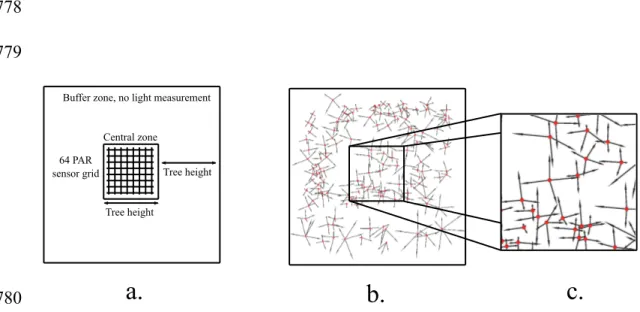
2. Canopy structure measurements
159
All trees in a square area, the experimental unit (Fig.1a), of size approximately 160
three times the height of dominant trees, were identified (species), located by their 161
x, y coordinates, and measured for their total height and Diameter at Breast Height 162
(DBH). Top and bottom crown heights were also measured. Lateral crown extents 163
was assessed by visually projecting to the soil its characteristic points (i.e. the 164
points that better describe the crown irregularities) in, at least, four directions, but 165
sometimes with more than 8 directions when necessary. The azimuth and distance 166
of those points from trunk were then measured (Fig.1b and c). 167
168
3. Light measurements
169
The light measurements were conducted in the central zone of the experimental 170
unit. The surrounding zone where dendrometric measures were done acts as a 171
buffer zone accounting for the attenuation of the encompassing forest (Fig.1a.). 172
The light measurements were achieved using a square grid composed of 64 PAR 173
sensors, namely Solems PAR/CBE 80 sensors. Each sensor was separated from its 174
neighbour in both direction by 2 to 3.5m depending on the considered plot (i.e. 175
depending on the mean size of the trees). This distance was set by previous 176
computation based on geostatistics (data not shown) and so that two contiguous 177
measurements (points) can be considered as independent. Light measurements 178
were done for each plot during 24h during summer to take the full sun course into 179
account. One additional PAR sensor, Sunshine sensor BF2, was positioned 180
outside of the experimental unit in full light to measure global (total) and diffuse 181
incident radiation. This extra sensor uses an array of photodiodes with a 182
computer-generated shading pattern to measure incident solar radiation and the 183
D/G ratio, i.e. the diffuse to global radiation ratio. Transmittance for each point in 184
the understorey is then computed as the ratio of light measured in the understorey 185
divided by the incident value. The D/G ratio is taken into account for simulating 186
the transmittance with the model. 187
188
4. Model description
189
Estimation of light transmission is a process that requires first the stand 190
reconstruction. Then, the light attenuation within each crown must be defined so 191
that the light model can compute the transmittance under the entire canopy. 192
1 Canopy reconstruction
193
From the dendrometric measurements on the field, a mockup of the stand is 194
generated. This generation involves the construction of a crown (and trunk) for 195
each tree of the stand and its positioning. To reconstruct the 3D envelopes of the 196
trees from the field measurements, we used the PlantGL library (Pradal et al. 197
2008). This library contains several geometric models, including different types of 198
envelopes and algorithms to reconstruct the geometry of plants at different scales. 199
In this work, we used the skinned surface which is a generalization of surface of 200
revolution with varying profiles being interpolated. The envelope of a skinned 201
hull is a closed skinned surface which interpolates a set of profiles {Pk, k = 0,...,
202
K} positioned at angle {2k , k = 0, . . . , K} around the z axis, where K is the
203
number of profiles used to generate the skinned surface. This surface is thus built 204
from any number of profiles with associated direction. In such case, a profile is 205
supposed to pass through common top and bottom points and at an intermediate 206
point of maximum radius, i.e. the height of the crown maximum width. Two 207
shape factors, CT and CB, were used to describe the shape of the profiles above
208
and below the maximum width. Mathematically, two quarters of super-ellipse of 209
degree CT and CB were used to define the top and bottom part of the profiles, see
210
Da Silva et al. (2008) for details. Note that our envelopes can be viewed as 211
extension of Cescatti (1997)'s asymmetric hull with profiles in any direction 212
instead of the restricted cardinal directions. Flexibility of our model enabled us to 213
measure the most adequate profiles in case of irregular crowns. The 3D envelope 214
of a tree was thus obtained using a skinned surface generated from profiles 215
defined from an angle, a maximum width and its associated height and two shapes 216
factors. The trunk of the tree was represented as a cylinder of DBH diameter, the 217
height of the cylinder being set to the crown bottom height. The 3D representation 218
of an experimental unit is presented in Fig.2. 219
1 Estimation of light transmission
220
The light transmission under such reconstructed stand was computed using the 221
multi-scale light interception model (M1SLIM) presented in Da Silva et al. 222
(2008). For each direction of incoming light, a set of beams was cast and the 223
attenuation of each beam through the canopy was estimated. In the present study, 224
the model was a simple two-scale model where the porous envelopes of crowns 225
constituted the finest scale and the stand, the coarser scale. In replacement of the 226
delicate estimation of leaf area density (LAD), a global opacity value, pgl, was
227
associated with each envelope of the reconstructed stand, the trunks were 228
considered opaque organs, thus their opacity was 1. Crowns global opacity were 229
estimated from field photographs shooting vertically different parts of the crown. 230
Each image was digitized, segmented to black and white and then the pixels were 231
counted using PiafPhotem software (Adam et al., 2006). The ratio of black pixels 232
to the total number of pixels yielded the opacity of the crown while the ratio of 233
white pixels to the total number of pixels produced the crown porosity, hence 234
porosity = 1 - opacity. However, the opacity of each individual crown was not 235
directly estimated using this method because the segmentation procedure still 236
required human intervention. Instead a global opacity value per species was 237
estimated over a sample of pictures (Tab.1). M1SLIM allowed then to compute 238
the light transmission of the canopy by considering the light attenuation of each 239
beam. The light attenuation for one beam is computed according to the opacities 240
of the crowns encountered along its trajectory and according to the path length 241
within each of these crowns. The porosity expression that takes the beam 242
travelling distance into account is related to G (Chen and Black 1992; Ross 1981; 243
Stenberg 2006), the extinction coefficient that depends on light direction and leaf 244
inclination distribution, and LAD, the leaf area density. It can be expressed as: 245
p2 13
4
b5 B
617exp67G.LAD.lb88, (1)
where B is the set of beams b, 3 is its cardinality, and lb is the path length of the
246
beam into the crown. To take this distance into account, we thus need to 247
determine the quantity G.LAD. 248
The global opacity value can be regarded as the result of opacity estimation using 249
Beer-Lambert law in a infinite horizontally homogeneous layer: 250 ) . exp( 1 G LAI pgl = − − . (2)
This relation yields an expression for G.LAI, where LAI is the leaf area index. In 251
the case of crowns with a finite volume, V, the usual definition of LAI can be 252
extended to be expressed as a function of the total leaf area, TLA, and the 253
projected envelope area, PEA (Sinoquet et al. 2007) 254
PEA TLA
LAI = , (3)
and since LAD is the ratio of total leaf area to crown volume, 255
V TLA
LAD = . (4)
We can express G.LAD as 256 V PEA p V PEA LAI G LAD G. = . . = −log(1− gl). . (5)
Using this G.LAD value with equation (1) naturally leads to a smaller envelope 257
opacity value than pgl. This is due to the fact that the negative exponential of a
258
mean value is less than the mean of negative exponential values. Therefore a 259
numerical approximation was carried out using the value from equation (5) as the 260
starting value to speed-up convergence. The process stopped when the opacity 261
computed using equation (1) was equal to the global opacity within a user-defined 262
error, 4. This G.LAD approximation was done once for each crown and for each 263
direction, and stored for further usage. The crown opacity for each beam, pb, was
264
then computed using the expression 265 ) . . exp( 1 b b G LAD l p = − − . (6)
The light transmission of the canopy along one direction was estimated by 266
computing, for each beam, its total opacity resulting from its travelling through 267
the canopy, i.e. possibly going through multiple crowns, see Da Silva et al. (2008) 268
for algorithmic and computational details. Experimental conditions were 269
simulated by using two sets of incoming radiation directions. The first set, for 270
diffuse light, discretized the sky hemisphere in 46 solid angle sectors of equal 271
area, according to the Turtle sky proposed by Den Dulk (1989). The directions 272
used were the central direction of each solid angle sector. The second set, for 273
direct light, was used to simulate the trajectory of the sun, and the directions were 274
dependant of the location (latitude, longitude), the day of the year, and on the time 275
step used for the sun course discretization (approx. 25 directions in this work). 276
Each of these directions was associated with a weighting coefficients derived from 277
the Standard Over Cast (SOC) distribution of sky radiance (Moon and Spencer 278
1942). The porosity is directly the ratio of transmitted light to incident light, a 279
value of 1 means that all light goes through while a value of 0 means that no light 280
goes through. The grey-level image constituted by the beam porosity values is 281
therefore a shadow map of the canopy transmittance. For each defined direction, 282
M1SLIM was used to compute the opacity values of the beams and to produce 283
such an image in a plane orthogonal to the light. To ensure both results precision 284
and fast computation, a lineic density of 150 was used for the beam sampling (Da 285
Silva et al., 2008), thus generating 150 x 150 pixels images. The images were 286
then projected on the ground and rotated according to the light directions azimuth. 287
Images from each set of incoming radiation directions were merged by using the 288
weighting coefficients producing two intermediate images, one for the integrated 289
transmittance of diffuse light and one for the direct light. Finally, these two 290
images were merged using the diffuse to total ratio, D/G, measured from the extra 291
sensor in the field. The grey-level values of pixels, from 0 (black) to 1 (white), 292
represented the transmittance classes simulated by M1SLIM. The simulated light 293
transmittance of the central zone could then be compared to the field 294 measurements. 295 296 5. Virtual experiments 297
To assess the effect of the deterioration of canopy description on the simulated 298
light histogram, we generated five different types of mockups for each stand with 299
decreasing amount of information on canopy architecture. 300
1. The asymmetric mockup where all available dendrometric data are used to 301
generate asymmetric crowns. 302
2. The simple mean mockup where crowns are represented by simple 303
geometric shapes, cones for pines, spheres otherwise, and where the radius 304
of each shape is the mean of the measured radii. 305
3. The simple max mockup where crowns are represented by simple 306
geometric shapes, cones for pines, spheres otherwise, and where the radius 307
of each shape is the maximum of the measured radii. 308
4. The allometric radius mockup where crowns are represented by simple 309
geometric shapes, cones for pines, spheres otherwise, and where the radius 310
of each shape is obtained from allometric relation with DBH. 311
5. The allometric mockup where crowns are represented by simple geometric 312
shapes, cones for pines, spheres otherwise, and where the radius of each 313
shape and the height of cones are obtained from allometric relation with 314
DBH.
315
For every type of mockup, the values for the height of crown base and for the 316
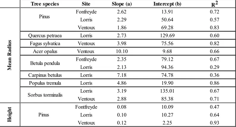
height of the cones (except for the allometric type) are the measured ones. 317
Allometric relations were defined as linear model between DBH and mean radius 318
and, for pines, between DBH and height. The relations obtained from field 319
measurements data are described in Tab.2, and Fig.2 shows 3D reconstructions 320
using two different types of crown shapes. 321
To complement the attenuation effect of the buffer zone for low elevation 322
radiations, it was necessary to add an artificial cylindrical wall surrounding the 323
zone of interest. The wall was centered on the zone of interest with a radius of the 324
zone of interest size. The height of the wall was set to the mean base crown height 325
of trees in the zone of interest. The coefficient of transmission of the wall (i.e. 326
wall opacity) was calibrated using in silico simulation experiments with the stands 327
of one site and then validated using the other stands from independent sites. 328
Adequacy of this method will be discussed further on. 329
330
6. Model estimation
331
The model outputs were qualitatively and quantitatively compared to experimental 332
data. The qualitative estimations were carried out by comparing the light 333
transmittance Cumulative Distribution Functions (CDF) to determine over- and/or 334
under-represented light transmittance class. The quantitative estimations were 335
achieved with the Kolmogorov–Smirnov test (K-S test) and the absolute 336
discrepancy index, AD (Gregorius 1974; Pommerening 2006). The K-S test is a 337
non-parametric test for the equality of continuous, one-dimensional probability 338
distributions that can be used to compare two samples. It quantifies the maximum 339
distance between the empirical CDF of two samples. The null distribution of this 340
statistic is calculated under the null hypothesis that the samples are drawn from 341
the same distribution. The p-value of the K-S test represents the 2 level at which 342
the null hypothesis can be rejected (i.e. a p-value > 0.1 means that the null 343
hypothesis cannot be rejected at 10% or lower level). 344
The absolute discrepancy index is defined as: 345
[ ]
01, 2 1 1 ' ∈ − =1
= AD s s AD n i i i (7)where n is the number of classes, si is the relative frequency in class i of the first
346
distribution, and s'i is the relative frequency in class i of the second distribution.
347
AD is defined as the relative proportion that needs to be exchanged between the 348
classes if the first distribution were to be transformed into the second distribution. 349
Correspondingly, 1-AD is the proportion common to both distributions, a value of 350
AD = 1 means that both distributions have no common class, whereas AD = 0 351
signifies that the distributions are absolutely identical (Pommerening 2006). 352
Both quantitative analysis were carried out with light measurements as reference 353
values and the results are shown in Tab.3. 354
355
Results
356
The comparison between the CDF of the measured light transmittance and the 357
ones obtained with the different mockups, as shown in Fig.3, were used to 358
qualitatively assess the quality of the model prediction and the effect of 359
deterioration of crown shape description. The CDF provides an alternate 360
representation to light transmittance histograms that facilitates comparison 361
between different distributions. The importance of a specific light transmittance 362
class is given by the slope of the CDF at that point, i.e. a non represented class 363
will yield a null slope and the more substantial the class, the steeper the slope 364
(Fig. 3). The classes of high importance will be titled as main classes whereas the 365
classes of low significance will be designated as minor classes. 366
367
Simulation with asymmetric mockups
368
The light model using the asymmetric mockups was able to simulate light 369
transmission distribution similar to the measurement with a level of confidence of 370
the K-S test above 5% for all stands except Fonfreyde5 (3%) and Fonfreyde1 371
(<1%). In that case, the mean comparison yielded a statistically significant 372
difference for the same two stands. However, the AD values were below 0.3 for 373
all stands with a mean of 0.21 (Tab.3). 374
In the case of Fonfreyde1, the measured transmitted light were almost evenly 375
distributed in only two light transmittance classes, [0-5] and [5-10]. The simulated 376
distribution showed the same two main classes with an unbalance in favor of the 377
[0-5] class. Although the p-value of the K-S test allowed to reject the hypothesis 378
that the measured and simulated light distribution were similar, the AD value was 379
below the mean value of all stands. The simulated transmittance of Fonfreyde2 380
were almost identical to the measured ones despite the missing [0-5] class in the 381
simulation (i.e. simulated CDF slope is null through entire [0-5] class). The best 382
values for both the p-value and AD were obtained for this stand. In the case of 383
Fonfreyde3 the difference in the standard deviation (Tab.3) between the measured 384
and simulated light distributions was a good indicator of the fact that the lower 385
and higher classes, [15-25] and [50-60] respectively, were not simulated to the 386
profit of the median classes [30-40] as shown by the Asymmetric CDF being 387
below and then above the CDF of measurements. On the contrary, in the case of 388
Fonfreyde5, the Asymmetric CDF started below and ended above the 389
measurement one, indicating that the median classes ([10-20]) were under 390
simulated to the benefit of the [30-35] class that did not appear in the 391
measurements and the [5-10] one that have very low substance. The highest AD 392
values were obtained for these two stands. 393
The simulated distributions for Lorris38 correctly rendered both the main and 394
minor classes with, however, a less pronounced peak for the [5-10] class 395
expressed by the more abrupt slope of the measured CDF. There were no missing 396
or extra classes simulated and the AD was just above the mean value. Similarly to 397
Lorris38, the main and minor classes of Lorris255 were correctly simulated 398
without any missing or extra classes. Within each group, main and minor, some 399
classes were under-represented to the benefit of the over-represented ones. 400
However these discrepancies were subsidiary as the very high p-value and the 401
below-the-mean AD attest. In the case of VentouxC7, the simulated distribution 402
reproduced the bell-shape of the measured one but with slightly heavier tails due 403
to the two extra classes on the sides of the distribution, [35-40] and [65-70]. Note 404
that the isolated [10-15] measured class was not simulated, as shown by the 405
advent of a proportion difference between measurements and simulation. 406
Similarly to Lorris255, a high p-value and a low AD were observed despite of 407
these differences. Finally, the simulated distribution for Ventoux34, whereas 408
correctly simulating the two main classes, [0-5] and [5-10] accounting for almost 409
70% of the transmittance distribution, increased the unbalance between them in 410
favor of the lowest one. The minor classes were adequately simulated but without 411
respecting the discontinuity shown in the measurements as indicated by the above-412
mean AD. 413
Simulation with the simple mean mockups
415
Replacing the asymmetric by the simple mean mockups significantly reduced the 416
p-values of the KS test, except for Fonfreyde1 and Fonfreyde3, but yielded AD 417
values below 0.3, except for Fonfreyde5 and VentouxC7, that were similar to the 418
ones obtained with the asymmetric mockups as shown by the slight increase of the 419
mean AD to 0.24. The principal effect of this change of crown shape on the 420
distributions of light transmittance compared to the distributions obtained with the 421
asymmetric crowns was to reduce the most represented classes to the benefit of
422
the minor ones. This was comparable to the crushing effect obtained on a 423
Gaussian function by increasing its variance parameter. The variance increase was 424
indeed observed for all stands but Lorris255 and interestingly, the two sample t-425
test indicated statistically significant differences for Fonfreyde5, VentouxC7 and 426
Lorris255. This effect actually benefited Fonfreyde1, Fonfreyde3 and Lorris38 427
simulation results. The p-value increased and AD decreased significantly for 428
Fonfreyde1 and Fonfreyde3, whereas for Lorris38, both values decreased. 429
430
Simulation with the simple max mockups
431
The simple max approach yielded light transmittance distributions that were 432
significantly shifted to the lower transmittance classes, i.e. left shifted CDF (Fig. 433
3). This effect was visible on the simulation results of all stands but was less 434
pronounced for Fonfreyde3 and VentouxC7. The dramatic increase of the AD 435
mean value to 0.6 well illustrated this behavior but mean comparison was 436
sufficient to assess the importance of the discrepancies. 437
438
Simulation with allometric mockups
439
The use of the allometric radius and allometric mockups yielded similar results as 440
illustrated by comparable means and variances and similar mean AD values, 0.345 441
and 0.333, respectively. The effect of this change of crown shape on the 442
distributions of light transmittance was similar to the simple mean effect with the 443
addition of a slight shift toward higher transmittance classes, indicated by right 444
shifted CDF (Fig. 3). The p-values were significantly reduced except for 445
Fonfreyde1, Fonfreyde5 and Ventoux34, but only for Fonfreyde1 this increase of 446
the p-value was associated with a decrease of AD (Tab.3). 447
448
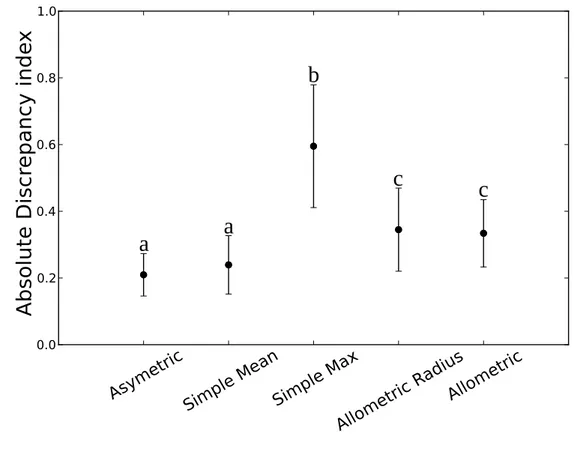
Comparison between all simulations
449
The AD results (Fig.4) show that the asymmetric mockups yielded the 450
distributions closest to the measurement, the simple mean approach deteriorated 451
slightly the results whereas the simple max approach had dramatic effect. Using 452
allometric crowns yielded results in between but closer to the simple mean ones.
453
These results confirmed the classification trend yielded by the two-sample t-test 454
analysis that showed no statistically significant differences between the 455
measurements and the asymmetric and simple mean approaches on one side, 456
between the two allometric approaches on the other side and showed the 457
segregation of the simple max one. 458
459
Discussion
460 461 Statistical considering 462Our study on the impact of the deterioration of the accuracy of crown 463
representation on simulated light transmission highlighted some statistical issues. 464
In spatially explicit transmittance models, a spatially point to point comparison 465
approach between measured and modeled transmittance generally shows little 466
agreement because small errors in crown location, often coming from errors 467
during field measurements, yields large local differences in transmittance 468
(Mariscal et al. 2004), particularly when the proportion of direct radiation is 469
important (Groot et al. 2004). However only considering a mean and variation 470
around this mean (e.g. SD) could lead to some errors (e.g. underestimation of area 471
fully lighted) due to distribution non centered on mean with sometimes a long tail 472
or several modes. To avoid this problem we compared the simulated distribution 473
of light transmittance to the measured ones using two different non parametric 474
descriptors, the K-S test and the AD index. 475
Although commonly used, and mathematically well-founded, the K-S test showed 476
some limitations when applied to peculiar distributions as the one from 477
Fonfreyde1. The problem stems directly from the test definition where the 478
accordance between two distributions is based on the maximum distance between 479
the CDFs. When the distribution shows very low dispersion, a small difference in 480
distribution can yield a big maximum distance between CDFs and therefore a 481
rejection of the null-hypothesis from K-S test. On the contrary, the AD index that 482
measures the changes required to transform one distribution into the other is 483
robust in regard of the distribution dispersion. Even though AD is very well suited 484
to quantify the difference between distributions or to classify results, the AD value 485
is not associated with any confidence index. Hence it is up to the user to define the 486
threshold under which distributions will be considered similar. Consequently, 487
combining the use of the K-S test and the AD index allowed us to accurately 488
compare and assess the differences between simulated and measured light 489 distributions. 490 491 Model evaluation 492
The goal of the present study was not to validate, stricto sensus, the model 493
MµSLIM. Such an evaluation would require an independent data set of light and 494
tree measurements. Our objective was to evaluate the quality of light predictions 495
with increasing deterioration of the crown description. However the comparison 496
of light measurements (with 64 sensors regularly distributed on a square grid in 497
the plot) and the simulation with full asymmetric crown description (i.e. crown 498
radius extension in 4 to 8 directions + crown height and length) showed the good 499
quality of simulated light distribution (K-S p-value > 0.10 or AD <0.3). Results 500
are in the range of models using similar scales of description (e.g. Brunner 1998; 501
Cescatti 1997; Gersonde et al. 2004; Groot 2004; Mariscal et al. 2004; Stadt and 502
Lieffers 2000). 503
As pointed out by Norman and Welles (1983), the computation of beam path 504
lengths is a crucial procedure. Due to the multi-scale design of MµSLIM, in 505
addition to the possibility of using any type of envelope, an analytical resolution 506
as proposed by Norman and Welles (1983) or Cescatti (1997) was not an option. 507
This task was instead performed by ray tracing algorithms that determine and 508
analyse the path of each cast ray among the canopy crown shapes (Wang and 509
Jarvis, 1990). With the ever increasing computational power of graphic cards 510
available to high level operations, this formerly time consuming procedure can 511
now be executed for many direction without impairing the model performances. 512
513
To avoid the problem of low elevation angles ; i.e. interception of light by very far 514
elements close to the horizon in the field, whereas not represented in the model, 515
we had to come up with an alternative to the classical solution of canopy 516
duplication or projection on torus. These approaches are based on the strong 517
assumption of canopy homogeneity ; using them with our strongly heterogeneous 518
stands would introduce a non controlled approximation that would, in turn, induce 519
bias in the results interpretation. Instead we chose to estimate the radiative 520
parameters of the surrounding environment using an inverse modeling approach 521
through the addition of an opaque wall. The wall opacity was calibrated using 522
Fonfreyde stands data with full asymmetric crown description. The value was then 523
used as a parameter to run the simulations for the stands from the two other 524
independent sites at the same level of crown description. Finally, the model 525
predictions were compared to the field light measurements. The results suggest 526
that the coefficient of transmission of the wall properly represented the radiative 527
properties of the environment, at least for low elevation angles. Moreover, 528
considering our objective, the opaque wall approach provided a simple solution 529
saving significant computational time otherwise required by the canopy 530
duplication. This approach seems thus promising and simple to set-up but would 531
benefit from more complete sensitivity analysis, in particular on wall size or 532
position. 533
One interest of our model is that crown porosity is simply estimated by a vertical 534
photograph of tree crown (extension of the method of Canham et al. 1999) and 535
seems to support accurate results in light distribution; however the extent to which 536
this parameter influenced the results needs to be more adequately studied. As 537
pointed out by Stadt and Lieffers (2000) determination of leaf and shading 538
elements (branch, trunk) is often critical in light transmission modeling. 539
540
Effects of crown description deterioration
541
Our results corroborate that differences in crown shape and size is a key 542
determinant of light transmittance as stated by Vieilledent et al. (2010). Moreover, 543
this study confirmed the importance of crown shape when simulating spatialized 544
light transmittance and endorse the sensitivity to variations in the crown geometry 545
parameters, especially the crown radius parameter, as already reported (Beaudet et 546
al. 2002; Brunner 1998; Cescatti 1997). However a crown mean radius with
547
crown height and spatialization seem to be a good alternate (Courbaud et al. 2003) 548
to detailed measures (i.e. measurement of crown extension in 4 to 8 directions) 549
even though simple shape like spheres and cones are known to be inadequate 550
(Mariscal et al. 2004). Other shapes should be tested, more in relation with tree 551
species architecture. Simplifying the crown representation in the tRAYci model to 552
average values for species and canopy strata resulted in little reduction in the 553
model performance (Gersonde et al. 2004). Describing tree crown extension with 554
4 to 8 radius is typically non feasible in practice in management or inventory 555
operations, whereas assessing mean crown diameter may be acceptable in some 556
cases. Therefore an approach that starts with simple shapes that can later be 557
deformed using an optimization process (Boudon and Le Moguedec 2007; Piboule 558
et al. 2005) should be considered in further studies. Indeed previous studies
559
showed the importance of crown asymmetric plasticity in response to local light 560
availability and space, among other factors (Vieilledent et al. 2010 and references 561
in it). 562
563
However using an Allometric approach would be more comfortable. The problem 564
is that the use of relationships between tree DBH and crown diameter or crown 565
height often decreased transmittance distribution prediction, whereas not for all 566
stands. With the allometric approach, the model generated smaller crown than 567
simple mean, thus same effect with shift to higher transmittance. We only tested
linear relationships and non-linear functions could have led to slightly better 569
results (Beaudet et al. 2002) ; however many authors pointed out that the 570
predictive functions for crown radius from e.g. DBH has proved elusive (Stadt et 571
al. 2000) as they are often highly affected by uncontrolled factors such as climate
572
hazards, stand density, or thinning operations (as probably reflected in the 573
Fontfreyde's plots). There is often a high variability in tree allometry from an 574
individual to another (Vieilledent et al. 2010). Actually the R² of the relationships 575
linking crown diameter to trunk diameter in that study are not excellent but in the 576
range of those commonly found in other studies (e.g. about 0.7 in Pinno et al. 577
2001 or Pukkala et al. 1993). 578
579
Effects of the stand complexity
580
High light variability is generally recorded in forests due to temporal variations of 581
the sun path and heterogeneous spatial arrangement of light intercepting elements 582
in irregular and/or mixed stands (Courbaud et al. 2003; Pukkala et al. 1993). In 583
stands with a clumped structure (i.e. tree clumps alternating with large gaps), only 584
an approach at tree scale with spatialization can correctly predict transmittance, 585
whereas in dense stands, a Beer-Lambert law can be applied at the stand canopy 586
scale (Balandier et al., 2010). It is however important to note that in dense stands, 587
importance of small gaps within tree crowns due to different causes (diseases, 588
broken branches, not taken into account in the simulation) can lead to noticeable 589
differences as such of Fontfreyde 1 (Fig.3) (Beaudet et al. 2002). Low density 590
stands Fonfreyde3 and VentouxC7 are less affected by the simple max approach 591
probably because the crown “increase” is not enough to fill the 'big' gaps in the 592
canopy. Problems of crown overlaps, in fact very difficult to quantify in the field, 593
are also probably less critical than in dense stands. 594
As already pointed out by Courbaud et al. (2003) or Balandier et al. (2010) the 595
problem is that it is very difficult to generalize results recorded on a site for a 596
particular stand structure to other sites or stands with other species or structures. 597
This argues in favor of studying the effect of stand structure in interaction with the 598
scale of stand description; this could be done for instance by the use of point 599 process analysis. 600 601
Acknowledgements
602The authors would like to thank for their help, in the field or for information on 603
the stands, Catherine Menuet, Gwenael Philippe, Philippe Dreyfus, and Yann 604 Dumas. 605 606
Funding
607The study was partly supported by the French program “ECOGER”, sustainable 608
management of mixed forests. 609
610
References
611
Adam B, Benoît JC, Balandier P, Marquier A, Sinoquet H (2006) PiafPhotem - 612
software for thresholding hemispherical photographs. Version 1.0. UMR PIAF 613
INRA-UBP, Clermont-Ferrand - ALLIANCE VISION Montélimar, France. 614
615
Balandier P, Collet C, Miller JH, Reynolds PE, Zedacker SM (2006a) Designing 616
forest vegetation management strategies based on the mechanisms and dynamics 617
of crop tree competition by neighbouring vegetation. Forestry 79, 1: 3-27. 618
619
Balandier P, Marquier A, Dumas Y, Gaudio N, Philippe G, Da Silva D, Adam B, 620
Ginisty C, Sinoquet H (2009) Light sharing among different forest strata for 621
sustainable management of vegetation and regeneration. In: Orlovic S (ed) 622
Forestry in achieving millennium goals, Institute of lowland forestry and 623
environment, Novi-Sad, Serbia, pp 81-86. 624
625
Balandier P, Marquier A, Perret S, Collet C, Courbeau B (2010) Comment estimer 626
la lumière dans le sous-bois forestier à partir des caractéristiques dendrométriques 627
des peuplements. Rendez-Vous Techniques ONF 27-28: 52-58. 628
629
Balandier P, Sonohat G, Sinoquet H, Varlet-Grancher C, Dumas Y (2006b) 630
Characterisation, prediction and relationships between different wavebands of 631
solar radiation transmitted in the understorey of even-aged oak (Quercus petraea, 632
Q. robur) stands. Trees 20: 363-370.
633 634
Bartelink HH (1998) Radiation interception by forest trees: a simulation study on 635
effects of stand density and foliage clustering on absorption and transmission. 636
Ecol Model 105: 213-225. 637
638
Beaudet M, Messier C, Canham C (2002) Predictions of understorey light 639
conditions in northern hardwood forests following parameterization, sensitivity 640
analysis, and tests of the SORTIE light model. For Ecol Manage 165: 235-248. 641
642
Boudon F, Le Moguedec G (2007) Déformation asymétrique de houppiers pour la 643
génération de représentations paysagères réalistes. Revue Electronique 644
Francophone d'Informatique Graphique (REFIG) 1, 1. 645
646
Brunner A (1998) A light model for spatially explicit forest stand models. For 647
Ecol Manage 107: 19-46. 648
649
Canham C, Coates KD, Bartemucci P, Quaglia S (1999) Measurement and 650
modeling of spatially explicit variation in light transmission through interior 651
cedar-hemlock forests of British Columbia. Can J For Res 29: 1775-1783. 652
653
Cescatti A (1997) Modelling the radiative transfer in discontinuous canopies of 654
asymmetric crowns. I. Model structure and algorithms. Ecol Model 101: 263-274. 655
Cescatti A (1997) Modelling the radiative transfer in discontinuous canopies of 657
asymmetric crowns. II. Model testing and application in a Norway spruce stand. 658
Ecol Model 101: 275-284. 659
660
Chen JM, Black TA (1992) Defining leaf area index for non-flat leaves. Plant Cell 661
Env 15: 421-429. 662
663
Courbaud B, de Coligny F, Cordonnier T (2003) Simulating radiation distribution 664
in a heterogeneous Norway spruce forest on a slope. Agr For Meteor 116: 1-18. 665
666
Da Silva D (2008) Caractérisation de la nature multi-échelles des plantes par des 667
outils de l'analyse fractale, application à la modélisation de l'interception de la 668
lumière. Dissertation, University of Montpellier, France. 669
670
Da Silva D, Boudon F, Godin C, Sinoquet H (2008) Multiscale Framework for 671
Modeling and Analyzing Light Interception by Trees. Multiscale Modeling & 672
Simulation 7: 910-933. 673
674
Den Dulk JA (1989) The interpretation of Remote Sensing, a feasibility study. 675
Dissertation, University of Wageningen, The Netherlands. 676
677
Gaudio N, Balandier P, Dumas Y, Ginisty C (2011) Growth and morphology of 678
three forest understorey species (Calluna vulgaris, Molinia caerulea and 679
Pteridium aquilinum) according to light availability. For Ecol Manage 261:
489-680
498. 681
682
Gersonde R, Battles JJ, O'Hara KL (2004) Characterizing the light environment in 683
Sierra Nevada mixed-conifer forests using a spatially explicit light model. Can J 684
For Res 34: 1332-1342. 685
686
Gregorius HR (1974) Genetischer Abstand zwischen Populationen. I. Zur 687
Konzeption der genetischen Abstandsmessung (Genetic distance among 688
populations. I. Towards a concept of genetic distance measurement). Silvae 689
Genetica 23: 22-27. 690
691
Groot A (2004) A model to estimate light interception by tree crowns, applied to 692
black spruce. Can J For Res 34: 788-799. 693
694
Hale SE, Edwards C, Mason WL, Price M, Peace A (2009) Relationships between 695
canopy transmittance and stand parameters in Sitka spruce and Scots pine stands 696
in Britain. Forestry 82, 5: 503-513. 697
698
Lieffers VJ, Messier C, Stadt KJ, Gendron F, Comeau PG (1999) Predicting and 699
managing light in the understory of boreal forests. Can J For Res 29: 796-811. 700
701
Mariscal MJ, Martens SN, Ustin SL, Chen J, Weiss SB, Roberts DA (2004) Light-702
transmission profiles in an old-growth forest canopy: simulation of 703
photosynthetically active radiation by using spatially explicit radiative transfer 704
models. Ecosystems 7: 454-467. 705
706
Monsi M, Saeki T (1953) Uber den Lichtfaktor in den Pflanzengesellschaften und 707
seine Bedeutung fur die Stoffproduktion. Japanese Journal of Botany 14: 22-52 708
709
Moon P, Spencer DE (1942) Illumination from a non-uniform sky. Transactions 710
of the Illumination Engineering Society 37. 711
712
Myneni RB, Ross J, Asrar G (1989) A review on the theory of photon transport in 713
leaf canopies. Agr For Meteor 45:1-153 714
715
Norman J.M., Welles J.M. (1983) Radiative Transfer in an array of Canopies. 716
Agronomy Journal 75: 481-488. 717
718
Perrin H (1963) Sylviculture. Ecole Nationale des Eaux et des Forêts, Nancy, 719
France, Tome 1, p 174. 720
721
Pinno BD, Lieffers VJ, Stadt KJ (2001) Measuring and modelling the crown and 722
light transmission characteristics of juvenile aspen. Can J For Res 31: 1930-1939. 723
724
Pommerening A (2006) Evaluating structural indices by reversing forest structural 725
analysis. For Ecol Manage 224: 266-277. 726
727
Pradal C, Dufour-Kowalski S, Boudon F, Fournier C, Godin C (2008) OpenAlea: 728
a visual programming and component-based software platform for plant 729
modelling. Funct Plant Biol 35. 730
731
Pukkala T, Kuuluvainen T, Stenberg P (1993) Below-canopy distribution of 732
photosynthetically active radiation and its relation to seedling growth in a boreal 733
Pinus sylvestris stand. Scand J For Res 8: 313-325. 734
735
Ross J (1981) The radiation regime and the architecture of plant stands. The 736
Hague, The Netherlands. 737
738
Sillion FX, Puech C (1994) Radiosity and Global Illumination. The Morgan 739
Kaufmann Series in Computer Graphics, Morgan Kaufmann Inc. San Francisco, 740
California, USA 741
742
Sinoquet H, Stephan J, Sonohat G, Lauri PE, Monney P (2007) Simple equations 743
to estimate light interception by isolated trees from canopy structure features: 744
assessment with three-dimensional digitized apple trees. New Phytol 175: 94-106. 745
746
Song C, Band LE (2004) MVP: a model to simulate the spatial patterns of 747
photosynthetically active radiation under discrete forest canopies. Can J For Res 748
34: 1192-1203. 749
750
Sonohat G, Balandier P, Ruchaud F (2004) Predicting solar radiation 751
transmittance in the understory of even-aged coniferous stands in temperate 752
forests. Ann For Sci 61: 629-641. 753
754
Stadt KJ, Lieffers VJ (2000) MIXLIGHT: a flexible light transmission model for 755
mixed-species forest stands. Agr For Meteor 102: 235-252. 756
757
Stenberg P (2006) A note on the G-function for needle leaf canopies. Agr For 758
Meteor 136: 76-79. 759
760
Tardieu F (2010). Why work and discuss the basic principles of plant modeling 50 761
years after the first plant models? J. Exp. Bot., 61:2039-2041. 762
763
Vieilledent G, Courbaud B, Kunstler G, Dhôte JF, Clark JS (2010) Individual 764
variability in tree allometry determines light resource allocation in forest 765
ecosystems: a hierarchical Bayesian approach. Oecologia 163: 759-773. 766
767
Wang YP, and Jarvis PG (1990) Description and validationof an array model - 768
MAESTRO. Agr For. Meteor 51: 257-280. 769
38 of 44
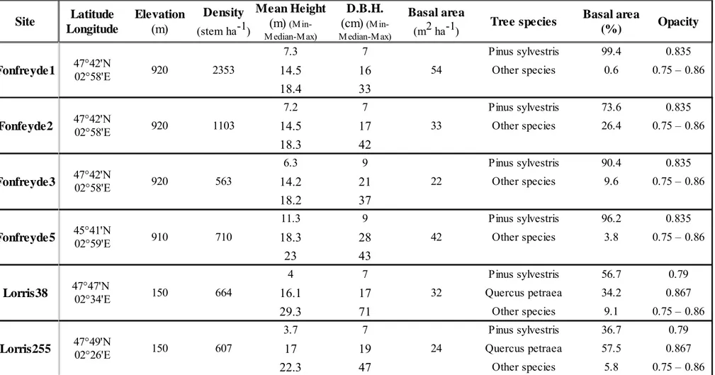
Tables
770 771 772 773Table 1: Plot description. Each plot was approximately 50m x 50m
Site Tree species Opacity
Fonfreyde1 920 2353 7.3 7 54 Pinus sylvestris 99.4 0.835 14.5 16 Other species 0.6 0.75 – 0.86 18.4 33 Fonfeyde2 920 1103 7.2 7 33 Pinus sylvestris 73.6 0.835 14.5 17 Other species 26.4 0.75 – 0.86 18.3 42 Fonfreyde3 920 563 6.3 9 22 Pinus sylvestris 90.4 0.835 14.2 21 Other species 9.6 0.75 – 0.86 18.2 37 Fonfreyde5 910 710 11.3 9 42 Pinus sylvestris 96.2 0.835 18.3 28 Other species 3.8 0.75 – 0.86 23 43 Lorris38 150 664 4 7 32 Pinus sylvestris 56.7 0.79 16.1 17 Quercus petraea 34.2 0.867 29.3 71 Other species 9.1 0.75 – 0.86 Lorris255 150 607 3.7 7 24 Pinus sylvestris 36.7 0.79 17 19 Quercus petraea 57.5 0.867 Latitude Longitude Elevation (m) Density (stem ha-1) Mean Height (m) (Min-Median-Max) D.B.H. (cm) (Min-Median-Max) Basal area (m2 ha-1) Basal area (%) 47°42'N 02°58'E 47°42'N 02°58'E 47°42'N 02°58'E 45°41'N 02°59'E 47°47'N 02°34'E 47°49'N 02°26'E
774 775
Table 2: Allometric relation between DBH and crown mean radius and height. Linear models of the form
a*DBH + b were used for both mean radius and height
Tree species Site Slope (a) Intercept (b)
M ea n R a d iu s Fonfreyde 2.62 13.91 0.72 Lorris 2.29 50.64 0.57 Ventoux 1.86 69.28 0.83
Quercus petraea Lorris 2.73 129.69 0.60
Fagus sylvatica Ventoux 3.98 75.56 0.82
Acer opalus Ventoux 10.10 9.68 0.66
Betula pendula Fonfreyde 2.35 79.12 0.67
Lorris 2.13 94.36 0.29
Carpinus betulus Lorris 7.18 74.78 0.36
Populus tremula Lorris 4.86 19.90 0.86
Sorbus torminalis Lorris 3.19 135.01 0.67
Ventoux 2.88 85.38 0.71 H ei g h t Pinus Fontfreyde 0.08 10.09 0.47 Lorris 0.10 10.27 0.64 Ventoux 0.12 2.25 0.93 R2 Pinus
40 of 44 776
Table 3 Simulation results for the different mockups reconstruction. The p-value of the K-S test and the absolute discrepancy index (AD)
were obtained with the measured light values as reference. Means with the same letter indicate that the difference between the means are not
statistically significant at 1=10% for an independent two-sample t-test.
Stand\Mockup Measures Asymmetric Simple Mean Simple Max Allometric Radius Allometric
F o n fr ey d e1 Mean Std 1.3 1.71 2.41 0.57 2 2.02 p-value 1.3e-5 9.8e-3 <1e-5 7.1e-5 3.1e-5
AD 0.203 0.063 0.516 0.141 0.172 F o n fr ey d e2 Mean Std 3.58 3.18 4.62 3.14 4.18 3.89 p-value 0.987 0.05 <1e-5 <1e-5 <1e-5
AD 0.078 0.219 0.75 0.594 0.531 F o n fr ey d e3 Mean Std 9.46 5.73 8.66 9.3 7.71 7.35 p-value 0.08 0.52 <1e-5 1.3e-5 9.8e-3
AD 0.281 0.234 0.453 0.406 0.329 F o n fr ey d e5 Mean Std 4.37 6.68 7.94 6.35 7.43 8.32 p-value 0.03 0.017 <1e-5 9.8e-3 0.05 AD 0.281 0.344 0.578 0.406 0.406 L o rr is 3 8 Mean Std 6.85 5.54 5.99 1.31 7.66 7.91 p-value 0.126 0.029 <1e-5 1.9e-5 <1e-5
AD 0.219 0.172 0.781 0.344 0.359 L o rr is 2 5 5 Mean Std 9.93 7.14 7.01 4.99 11.54 11.42 p-value 0.758 0.029 <1e-5 0.16 0.203 AD 0.172 0.25 0.844 0.281 0.266 V en to u x C 7 Mean Std 7.06 5.91 7.5 9.9 7.74 7.68 p-value 0.52 2e-4 7e-5 0.005 0.017
AD 0.172 0.359 0.375 0.266 0.281 en to u x 3 4 Mean Std 15.29 11.35 13.52 7.9 19.59 19.74 p-value 0.05 9.8e-3 <1e-5 0.274 0.188 5.15a 4.19b 5.06a 0.44c 4.29b 4.14b 14.7a 14.69a 15.72a 7.19c 21.37b 20.32b 38.08a,b 37.05a 39.58b 25.81c 48.09d 43.18e 16.89a 19.29b 18.87b,d 9.52c 16.81a,b,d 18.32a,d 8.43a 8.41a 8.61a 0.645c 15.79b 16.09b 20.8a 21.33a 25.36b 5.49c 21.1a 21.1a 53.34a 54.3a,b 57.38d 47.72c 55.66a,b 54.87b,d 12.25a,b 8.87a 10.54a 3.44c 16.85b 17.05b
Captions of Figures
777 778 779
780
Figure 1: a. Experimental Unit. b. Field data: each dot locates a tree (its trunk), and
each arrow defines a specific azimuth and distance from the trunk, characterizing
the crown extend. c. Zoom in on the interest zone where light measurements where
781
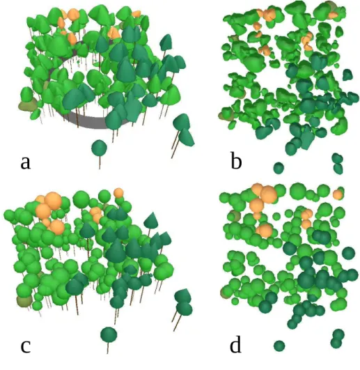
782 783 784
Figure 2: 3D reconstruction of the Lorris255 experimental unit using the
asymmetric crowns, side view(a) and top view(b), and using the crowns from the
allometric radius approach, side view(c) and top view(d) .Colors are used to
visually differentiate between tree species: dark green for pine (Pinus sylvestris L.),
green for oak (Quercus petraea L.), orange for birch (Betula L.), and brown for
786
787
Figure 3: Cumulative Distribution Function (CDF) of light transmittance for each
stand and for every mockup type. Note that for legibility purpose the x-axis scale
was adapted for each stand.
Figure 4: The points represent the mean of AD calculated for each type of mockup
over all stands, the bars being the standard deviation. Same letter above the bars
indicate that the difference between the means are not statistically significant at