HAL Id: hal-01229097
https://hal.archives-ouvertes.fr/hal-01229097
Submitted on 24 Nov 2015
HAL is a multi-disciplinary open access archive for the deposit and dissemination of sci-entific research documents, whether they are pub-lished or not. The documents may come from teaching and research institutions in France or abroad, or from public or private research centers.
L’archive ouverte pluridisciplinaire HAL, est destinée au dépôt et à la diffusion de documents scientifiques de niveau recherche, publiés ou non, émanant des établissements d’enseignement et de recherche français ou étrangers, des laboratoires publics ou privés.
Decentralized diagnosis in a spacecraft attitude
determination and control system
Carlos Gustavo Pérez, Louise Travé-Massuyès, Elodie Chanthery, Javier
Sotomayor
To cite this version:
Carlos Gustavo Pérez, Louise Travé-Massuyès, Elodie Chanthery, Javier Sotomayor. Decentralized di-agnosis in a spacecraft attitude determination and control system. Journal of Physics: Conference Se-ries, IOP Publishing, 2015, Conference SeSe-ries, 659, �10.1088/1742-6596/659/1/012054�. �hal-01229097�
Decentralized diagnosis in a spacecraft attitude
determination and control system
C G P´erez1,2,4, L Trav´e-Massuy`es1,3, E Chanthery1,4 and J Sotomayor2 1
CNRS, LAAS, 7 avenue du colonel Roche, F-31400 Toulouse, France
2
Pontificia Universidad Cat´olica del Per´u, Department of Engineering, Lima 32, Per´u
3
Universit´e de Toulouse, LAAS, F-31400 Toulouse, France
4
Universit´e de Toulouse, INSA, F-31400 Toulouse, France
E-mail: [email protected], [email protected], [email protected]. [email protected]
Abstract. In model-based diagnosis (MBD), structural models can provide useful information for fault diagnosis and fault-tolerant control design. In particular, they are known for supporting the design of analytical redundancy relations (ARRs) which are widely used to generate residuals for diagnosis. On the other hand, systems are increasingly complex whereby it is necessary to develop decentralized architectures to perform the diagnosis task. Decentralized diagnosis is of interest for on-board systems as a way to reduce computational costs or for large geographically distributed systems that require to minimizing data transfer. Decentralized solutions allow proper separation of industrial knowledge, provided that inputs and outputs are clearly defined. This paper builds on the results of [1] and proposes an optimized approach for decentralized fault-focused residual generation. It also introduce the concept of Fault-Driven Minimal Structurally-Overdetermined set (FMSO) ensuring minimal redundancy. The method decreases communication cost involved in decentralization with respect to the algorithm proposed in [1] while still maintaining the same isolation properties as the centralized approach as well as the isolation on request capability.
1. Introduction
With increasing complexity of industrial processes, the requirement for reliability, availability and security is growing significantly. Fault detection and isolation (FDI) are becoming a major issue in industry.
The structural approach constitutes a general framework to provide information when the system becomes complex. The main aim of the structural approach application is to identify the subsets of equations which include redundancy.
The system structure analysis, originally developed for the decomposition of large systems of equations for their hierarchical resolution, was adopted by the Fault Detection and Isolation (FDI) community [2, 3]. Structural concepts are used for analysis of system monitor ability using the concept of complete matching on a graph.
Decentralized diagnosis has received considerable attention to deal with distributed systems or with systems that may be too large to be diagnosed by one centralized site. In the same way, the decentralized solution allows proper separation of industrial knowledge, provided that inputs and outputs are clearly defined.
Decomposition has been recognized as an important leverage to manage architectural complexity of the systems to be diagnosed. Most of the approaches, however, focus on hierarchical decomposition [4], while decentralization has been explored less frequently. The majority of decentralized diagnosis methods concern discrete event systems [5, 6, 7]. In [6], the purpose of the method is to provide efficient online diagnosis to detect and isolate faults in large discrete event systems. [5] uses a decentralized approach to deal with the size of the model and to get a tractable representation of diagnosis. Along the same idea, [7] proposes a hierarchical framework that exploits different local decisions.
These ideas are taken into account for our approach of decentralization using the idea of isolation on request. If local diagnosis is not sufficient, a hierarchical architecture is built that allows for less ambiguous hierarchical diagnosis tests. Moreover, our proposal to use fault-driven residual generation targets decreasing computational effort.
Decentralized diagnosis methods have been applied only recently on continuous or hybrid systems. [4] presents a decentralized architecture for systems modeled in the qualitative framework. The architecture proposed is similar to that which is presented in this paper: the model of each subsystem is private and the supervisor needs no a-priori knowledge about the subsystems and their interactions. In addition, a multi-layered hierarchy of diagnosers is possible. This paper presents the design, in a decentralized architecture, of a fault-driven residual generation scheme bridging the algorithm for computing a Fault-Driven Minimal Structurally-Overdetermined (FMSO) set of subsystems. This paper is organized as follows: Section 2 introduces the basic concepts of analytical redundancy and presents the structural approach. Section 3 presents an approach for residual focus generation. Section 4 proposes an algorithm to generate the Decentralized Diagnoser based on FMSO. Section 5 illustrates the method proposed on the Attitude Determination and Control System (ADCS) of a LEO satellite. Finally, Section 6 discusses some conclusions and brings in current work.
2. Structural approach
In spite of their simplicity, structural models can provide much useful information for fault diagnosis and fault-tolerant control design. Structural analysis is able to identify those components of the system which are or are not able to be monitored, to provide design approaches for analytic redundancy based residuals, to suggest alarm filtering strategies, as well as to identify those components whose failure can be tolerated through reconfiguration [8].
The system structural model is an abstraction of its behavior in a sense that the structure of the constraints only considers links between variables and parameters and does not consider links between the constraints themselves. The links are represented by a bipartite graph, which is independent of the nature of the constraint (e.g. quantitative, qualitative, equations, rules, etc.), variables and parameters values [9]. It is important to summarize some structural concepts.
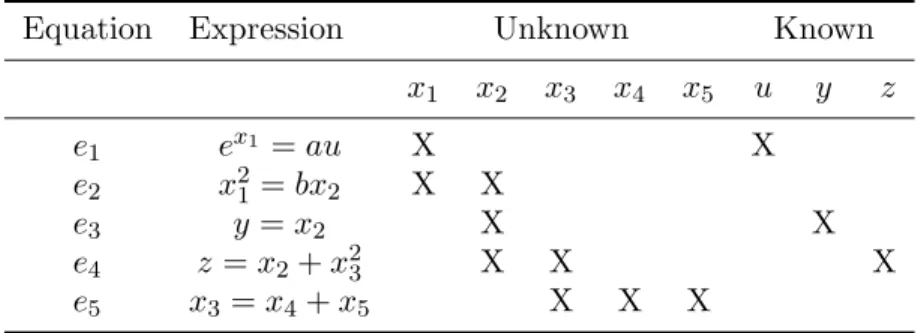
Definition 1 (Model): The behavior model of a system is denoted by M (z, x) or M for short, to be any set of equations relating the known variables z, i.e. measured variables, and the unknown variables x. The equations ei(z, x) ⊆ M (z, x), i = 1, ..., n are assumed to be differential
or algebraic equations in z and x, and the model is considered a differential-algebraic equation system. By example shown in Table 1, we illustrate the concepts introduced in this section. This is composed of five equations, e1 to e5, relating the unknown variables x = {x1, x2, x3, x4, x5}
and the known variables z = {u, y, z}.
Definition 2 (ARR for M(z,x)): The structure of a system is an abstract representation of which variables are involved in different equations and compose the model of the system. The structural abstraction allows us to derive redundancies disregarding the actual analytical expressions of equations making up the system model.
Let M (z, x) be a model. Then, a relation r(z, ˙z, ¨z, ...) = 0 is an Analytical Redundancy Relation (ARR) for M (z, x) if for each z consistent with M (z, x) the equation is fulfilled.
Table 1. Expressions and biadjacency matrix of an illustrative example.
Equation Expression Unknown Known
x1 x2 x3 x4 x5 u y z e1 ex1 = au X X e2 x21 = bx2 X X e3 y = x2 X X e4 z= x2+ x23 X X X e5 x3= x4+ x5 X X X
Obtaining ARRs for a model M (z, x) involves the elimination of unknown variables, which can be inferred from the bipartite graph. The bipartite graph actually represents which unknown variables are involved in the equations models of the system.
3. Fault-driven Residual Generation
In graph theory, a classical result from bi-partite graph states that any finite-dimensional graph can be decomposed into three subgraphs with specific properties by using the Dulmage-Mendelson (DM) canonical decomposition [10] as can be seen in Figure 1. The structurally over-determined part, represented by M+
, has more equations than variables; the structurally just-determined part, represented by M0
, has many equations than variables and the structurally under-determined part represented by M− has more variables than equations.
X− X0
X+ M−
M0
M+
Figure 1. Dulmage-Mendelson decomposition of M .
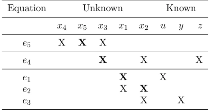
The biadjacency matrix in Figure 1, shows a DM canonical decomposition of a bipartite graph G(M ∪ X, A). The light blue-shaded areas contain ones and zeros, while the white areas only contains zeros. The thick line represents a maximal matching in the graph, where rows and columns are rearranged. For the example, by rearranging rows and columns, the DM decomposition is:
The bold X denotes a complete matching. The subsets for this example are: M− = {e5},
M0
= {e4}, M+= {e1, e2, e3}, X−= {x4, x5}, X0= {x3} and X+ = {x1, x2}.
The structural redundancy is used to define the ideas of structurally overdetermined (SO) set, proper structurally overdetermined (PSO) set and minimal structurally overdetermined (MSO) set. These ideas are therefore also compared to analytical redundancy [11].
Table 2. DM decomposition of illustrative example.
Equation Unknown Known
x4 x5 x3 x1 x2 u y z e5 X X X e4 X X X e1 X X e2 X X e3 X X
Definition 3 (Structurally overdetermined, SO): A set M of equations is SO if M has more equations that unknowns.
Definition 4 (Proper structurally overdetermined, PSO): A set of equations M is a PSO set if M = M+
. A PSO set is generically a testable subsystem but may contain smaller PSO subsets that are also testable subsystems [12]. The minimal PSO sets, called the MSO sets, are of special interest since these have the attractive properties of giving good isolation.
Definition 5 (Minimal structurally overdetermined, MSO): An SO set is a MSO set if no proper subset is also an SO set. Note that an MSO set is also a PSO set.
Structural methods have been used to perform isolation capability analysis and to find testable submodels (MSO sets). However, the number of MSO sets grows exponentially with the degree of redundancy making the task of computing MSO sets intractable for systems with high degree of redundancy. [13] introduces the concept of Test Equation Supports (TES), which is a set of equations expressing redundancy specific to a set of considered faults. The influence of faults is taken into account in the TES.
Let F (M ) denote the set of faults that influence any of the equations in M . Then, since a PSO set exactly characterizes a set of equations that can be used to form a test, a formal definition is then given by:
Definition 6 (Test Support, TS): Given a model M and a set of faults F , a subset of faults ζ ⊆ F is a test support if there exists a PSO set M′ ⊆ M such that F (M ) = ζ. Of special
interest are minimal test supports which are naturally defined as:
Definition 7 (Minimal Test Support, MTS): Given a model, a test support is a minimal test support (MTS) if no proper subset is a test support.
Definition 8 (Test Equation Support, TES): An equation set M is a Test Equation Support (TES) if: F (M ) 6= 0, M is PSO set and for any M′ + M where M′ is a PSO set it holds that
F(M′)+ F (M).
Also here it is interesting to consider minimal such sets of equations.
Definition 9 (Minimal Test Equation Support, MTES): A TES M is a minimal TES (MTES) if there exists no subset of M that is a TES.
Here it is clear that there is a one to one correspondence between a TES M and TS ζ given by the relation ζ = F (M )
An MSO set or MTES signifies the theoretical presence of a structural redundancy which can be used as a consistency check for a part of the system. It is important to notice that, whereas an MSO gives rise to one single residual generator, an MTES gathers all the equations leading to all the possible residual generators for the associated set of faults. Besides the fact that an MTES has a non empty TS, it represents a compact form for the whole set of MSOs sharing the
same TS.
Definition 10 (Fault Driven Minimal structurally overdetermined, FMSO): A FMSO is a minimal redundancy structurally overdetermined set of M focused on a minimal set of fault of interest. minimal|(F (M )|
The elements of a set of MTES can become FMSOs if they have a minimal redundancy. MTES does not guarantee the minimal redundancy sets so these sets will not always be the optimal sets to develop diagnosability.
4. Decentralized Diagnoser
This section introduces the ideas required to formalize decentralized ARR generation in a structural framework. In the following, the global level refers to no decentralization and, without loss of generality, we consider two hierarchical levels, the so-called local level and hierarchical level.
4.1. Fault-driven Decentralized Ideas
A decomposition of the system M , with associated bipartite graph G(M ∪ X ∪ Z, A), into several subsystems Mi is defined as a partition of its equations.
Let M = {M1, M2, ..., Mn} with Mi⊆ M : Mi 6=∅, n
S
i=1
Mi= M , Mi∩ Mj =∅ if i 6= j.
The decomposition of the global system leads to n subsystems denoted Mi(xlocali , zi), with
associated subgraphs G(Mi∪ Xilocal∪ Zi, Ai), i = 1, ..., n, Xilocal is defined below.
Definition 11 (Local Variables): The set of local variables of the ith subsystem, denoted
as Xlocal
i , is defined as the subset of vertices of Xi that are adjacent only to vertices in Mi and
not to vertices in any other subsystem Mj, j 6= i,
Xlocal
i = {u ∈ Xi :∄j(j 6= i), v ∈ Mj,(u, v) ∈ A}
Definition 12 (Shared Variables): The set of shared variables, denoted as Xshared are
defined as the subset of vertices of X that can not be considered local variables for any subsystem: Xshared= X \ n [ i=1 Xilocal ! (1) Consequently: ∀i ∈ {1, ..., .n}, Xlocal
i ∩ Xshared=∅.
The extensions of the ideas of FMSO and MSO at the local and the hierarchical level are first given below.
Definition 13 (Local FMSO): The set of local FMSO , denoted as Local FMSOi, is defined
as the subset of FMSO of the ith subsystem that are adjacent only to local variables in Mi and
not to shared variables in any other subsystem Mj, j 6= i,
Local FMSOi = {F M SO ∈ F M SOi :∄j(j 6= i), xshared∈ Mj}
Definition 14 (Shared FMSO): The set of Shared FMSO of the ith subsystem, is defined
as the subset of FMSO that can not be considered Local FMSO : Shared FMSOi = F M SOi\ n [ i=1 Local FMSOi ! (2) Consequently: ∀i ∈ {1, ..., .n}, Local FMSOi∩ Shared FMSOi=∅.
Definition 15 (Stored MSO): The set of Stored MSO, denoted as Stored MSOi, is defined
as the subset of MSO of the ith subsystem whose vertices Xm are adjacent to vertices Xn in
Definition 16 (Hierarchical FMSO): A set of hierarchical FMSO is a set of top level which includes the relations in Mi of the ith subsystem which are adjacent to the relations in
Shared FMSOi and Stored FMSOi sets for all corresponding subordinates subsystems.
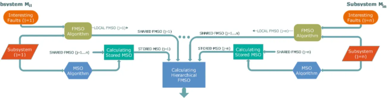
Figure 2 shows the scheme of the decentralized diagnoser proposed in this paper, for subsystems at level i of the diagnoser hierarchy. We consider two stages: the first one is offline for calculating analytical residual generators, and the second one is online and communicates directly with the system through a residual generator bank. In the following, we present the algorithm for calculating analytical residual generators in the first stage.
4.2. Algorithm
The diagnoser design is done offline and consists of the 6 steps below. These steps are performed for each subsystem Mi,j j = 1...ni at each level i = 1...nj, with a nested loop. Here i is the
level in the hierarchy, and j the enumeration of subsystems at the level. Figure 2 illustrates the proposed algorithm for level i.
Figure 2. Architecture of diagnoser offline
1) At the local level (level i), calculate the FMSO of the structural model for each subsystem Mi,j, considering shared variables as observed. Branch the results in two subsets.
Outputs:
• Local F M SO: for the subsystem Mi,j at level i.
• Shared F M SO: for the subsystem Mi,j at level i.
2) Still at local level i, compute the FMSO sets of the structural model for each subsystem Mi,j and store the set of equations (included in FMSO set) that share variables with Shared
FMSO of the other subsystem Mi,j.
Output:
• Stored MSO set for the subsystem Mi,j at level i to be sent at level i+1.
3) Send the Shared FMSO and Stored MSO sets to the hierarchical level.
4) Store the set of relations included in the Shared FMSO and the Stored MSO set for each subsystem Mi,j.
Output:
• Mi,j included Rel : relations included in the Shared FMSO and the Stored MSO set
for the each subsystem Mi,j as input at level i.
5) At the hierarchical level: compute the FMSO with the Mi,j included Rel of the all
subordinate local diagnosers of level i-1. Output:
• Hierarchical FMSO : FMSO of the relations included in the Shared FMSO and the Stored MSO for all subsystem subordinate local diagnosers of level i-1.
6) (optional) As a check, join the local F M SO and the hierarchical FMSO to find the FMSO computed for the global system in the centralized way.
Output:
• Global F M SO: local F M SO plus hierarchical FMSO.
In step one, the aim is find the Shared FMSO. Local FMSO are only involved in local redundancies and do not need to be analyzed in the upper hierarchical level. After the offline structural analysis, the diagnoser is implemented as a residual generator bank. With the system inputs/outputs, hierarchical and local residual generators are used online to detect and isolate faults at each level. Notice that, if a Shared FMSO or Stored MSO set is not sent at hierarchical level, it is possible that all MTES are not obtained.
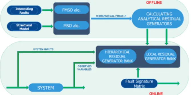
The offline / online FDI process is illustrated in Figure 3. Considering the system inputs and outputs, the hierarchical and local residual generators are used online to detect and isolate faults each level.
Figure 3. Scheme of a decentralized diagnoser for a subsystem at level i
4.3. The equivalence of centralized and decentralized diagnosis
It is desirable that properties such as detectability and isolation of faults are not altered by decentralization. This can be ensured if the set of FMSO derived with global and decentralized architectures are identical [1].
Proposition 1: The set of FMSO computed in a centralized way and the set of MTES computed in a decentralized way from the Stored MSO is the same.
Proof: Given a system decomposed into n subsystems denoted as {M1, M2, ..., Mn}. Let
{Local FMSOi, Shared FMSOi, Stored MSOi}, i = 1..n it is not necessary to send all MSO
because the necessary redundant information is in relationships that contain shared variables; i.e., the FMSO sets that share information with all Shared FMSO of the other subsystems. In the same way, the set of MTES computed in a centralized way and the set of MTES computed in a decentralized way ends the same, resulting in both case [1].
5. Application to the Attitude Determination and Control System of a LEO Satellite
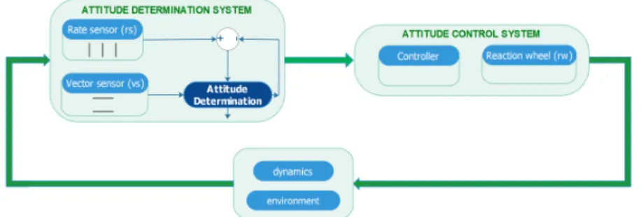
The decentralized diagnoser has been tested on the Attitude Determination and Control System (ADCS) of a low earth-orbit satellite. The composition of the ADCS of a typical satellite is represented in figure 4:
The attitude determination subsystem (ADS) is composed of sensors which sense the rate and angular position of the satellite. An attitude estimate is achieved using a sensor fusion (rate
Figure 4. Attitude Determination and Control System of a typical satellite
and vector sensors) [14], which is provided as input to the attitude control subsystem (ACS). The ACS is composed of the control signal calculation and the actuators which provide the stabilizing and/or control torque to the satellite. The satellite under study is assumed to be a three-axis stabilized satellite in orbit around the earth. Here, reaction wheels and magnetorquers are considered as actuators [15].
5.1. Dynamics of the satellite
To analyze the motion of the satellite, two sets of coordinate systems are defined: a Sun-centered inertial frame with its origin at the center of the Sun and its third axis (zi) normal to the ecliptic
plane of the rotation of the Earth around the Sun (xi, yi) and a body-fixed frame which has its
origin at the center of mass and its axes aligned with the principal axes of the satellite inertia. The satellite is modeled as a rigid body having the moments of inertia matrix along the principal axes of rotation, I=Diag3x3{Ix, Iy, Iz}. Assuming that xb, yb and zb are the principal
axes of inertia, the rotational motion of the satellite can be described in the body frame as follow [14]:
I ˙w= T − w × (Iw) (3)
where the angular velocity vector w has components wx, wy and wz, each along the body
axes xb, yb and zb of the satellite, ˙wis the angular acceleration, and T is the total torque acting
along the body axes. The system of differential equations describing the vehicle attitude is ˙ ψ ˙θ ˙ φ = 1 cθ 0 sφ cφ 0 cφcθ −sφcθ cθ sφsθ cφsθ wx wy wz (4)
where ψ, θ and φ denote yaw, pitch and roll angles, respectively. The state vector of the satellite is X = [ψ, θ, φ, ˙ψ, ˙θ, ˙φ]. They are the angles by which the body frame is rotated relative to a reference frame.
5.2. Attitude Determination and Control System modelling
The rate sensors of the satellite are three gyroscopes and the vector sensors are sun and star sensors. It is assumed that sensing axes of the rate gyros are aligned with each of the body axes of the satellite. The angular rate measurements from the gyros are used to solve the set of differential equations described by 4. wx,wy and wz represent outputs of the three orthogonal
rate gyros with their sensing axes aligned with the roll, pitch and yaw axes,respectively.
The attitude measurement from vector sensors is bounded and used to aid gyros to eliminate attitude drift error. The sensitive axes of the rate gyros are aligned with each of the body axes of the satellite. The modelling of the AD system is described in [14]. The vector and rate sensor
outputs are used to estimate the state vector both independently and merged together. These preliminary estimates are then fused together to arrive at the estimate which is feedback to the ACS. This redundancy can be used to check consistency [15].
The ACS is equipped with a three reaction wheels for 3-axis control. Another external torque source is necessary to unload the wheel’s angular momentum. For this satellite, magnetic torques are selected instead of thrusters that consume a large amount of fuel [16].
5.3. Fault scenarios
Faults are introduced in the system model equations. We consider faults occurring in the rate and vector sensors of the ADS and in the reaction wheels of the ACS. Each of these faults has three components corresponding to the three axes. The faults are summarized in Table 3.
Table 3. Fault scenarios of the ADCS.
Component Subsystem Fault
Vector sensors (vs) ADS fvs(fvsx, fvsy, fvsz)
Rate sensors (rs) ADS frs(frsx, frsy, frsz)
Reaction wheel (rw ) ACS frw(frwx, frwy, frwz)
5.4. Structural Model of the ADCS
The structure of the ADCS is abstracted as a set of constraints on a set of variables. Related information of such modelling can be founded in [16, 14]. Most constraints are composed of three behavioral relations corresponding to three axes. From the set of variables of the system, the sensed quantities form the set of observed variables with all the rest assumed to be unobserved. The general procedure for the diagnoser design starts with assuming a small set of observed quantities, and can be optionally expanded to fulfill diagnosis and isolation capability specifications.
The bi-adjacency matrix of the ADCS is shown in figure 5. The unobserved faults and observed variables are separeted along the X-axis. The constraints that describe the behavior of the system components are described on the Y-axis. The structural models of the ADCS, ADS and ACS are represented as (CADCS, XADCS, ZADCS),(CADS, XADS, ZADS) and (CADC, XADC, ZADC)
respectively. The structural model of the ADCS is composed of 42 constraints with 42 unobserved variables , 15 observed variables and 9 faults (modeled as variables in the bi-adjacency matrix).
The structural model of the satellite ADCS, is considered to demonstrate the proposed decentralized architecture while still maintaining the same isolation capability power as the centralized approach and the advantageous isolation on request capability.
5.5. Diagnoser Design
For reference, first we use the algorithm to determine MTS, MSO and FMSO sets to the ADCS considered globally. Constraints ei from 1 to n are denoted e1...en.
ADCS global diagnoser
Max fault isolability: [f rwx], [f rwy], [f rwz], [f rsx], [f rsy], [f rsz], [f vsx], [f vsy], [f vsz]
FMSO sets: [e4, e3, e10, e13], [e5, e8, e11, e14], [e6, e9, e12, e15], [e7...e21, e25], [e7...e21, e26],
Figure 5. ADCS structure of a LEO satellite.
Num. MSO sets: 2448
ACS local diagnoser (XSHARED unobserved)
Max fault isolability: [f rwx], [f rwy], [f rwz]
Local FMSO sets: [e4, e7, e10, e13], [e5, e8, e11, e14], [e6, e9, e12, e15]
ADS local diagnoser (XSHARED unobserved)
Max fault isolability: [f rsx, f vsx], [f rsy, f vsy], [f rsz, f vsz]
Local FMSO sets: [e22, e25, e28], [e23, e26, e29], [e24, e27, e30]
According to these results, it can be seen that all faults can be isolated with a centralized global diagnoser for the ADCS. However, for the local diagnoser ADS, faults on the rate and vector sensors can not be isolated locally. It also shows that between 2448 MSO sets and 9 FMSO sets there is a large computational advantage. Because MTES does not guarantee minimum redundancy, it has not been considered. It is more efficient to consider FMSO introduced in the previous section.
The proposed decentralized architecture will now be applied to the ADCS by designing the local and hierarchical diagnosers. It will be demonstrated that the isolation capability of such a decentralized diagnoser is equivalent to the global diagnoser above.
For each local diagnoser, the shared variables XSHARED are assumed to be observed. It
can be assumed that for each subsystem, shared variables are calculated in other local systems. Shared FMSO can be derived using the algorithm with this assumption.
ADS local diagnoser (XSHARED observed)
Max fault isolability: [f rsx], [f rsy], [f rsz], [f vsx], [f vsy], [f vsz]
Shared FMSO: [e19, e20, e21, e22, e28], [e19, e20, e21, e23, e29], [e19, e20, e21, e24, e30],
[e19, e20, e21, e25], [e19, e20, e21, e26], [e19, e20, e21, e27]
ACS local diagnoser (XSHARED observed)
Max fault isolability: [f rwx], [f rwy], [f rwz]
In the case of ACS local diagnoser, the results demonstrate the efficiency of FMSO sets to ensure minimal redundancy (sr = 1) compared with MTES sets: using the algorithm, as it dis-cussed in [1], the structural redundancy for this MTES set is equal to 10. Now, we can calculate the Hierarchical diagnoser with relations included in Shared FMSO and Stored MSO sets for every subsystem, this calculation its necessary to disambiguate faults.
ADCS Hierarchical diagnoser
Rel in Shared FMSO and Store MSO (ADCS) = [e1, e2, e3...e18], [e19, e20, e21...e30]
Fault isolability: [f rwx], [f rwy], [f rwz], [f rsx], [f rsy], [f rsz], [f vsx], [f vsy], [f vsz]
Hierarchical FMSO sets: [e4, e3, e10, e13], [e5, e8, e11, e14], [e6, e9, e12, e15], [e7...e21, e25],
[e7...e21, e26], [e7...e21, e27], [e7...e21, e22, e28], [e7...e21, e23, e29], [e7...e21, e24, e30]
Num. MSO sets: 2448
If we calculate the Hierarchical MTES sets, we can find the same sets because they have the minimal redundancy (sr = 1). However, they do not always have the same results because the MTES may have no minimum structural redundancy, which does not make them fully effective. 5.6. Simulation of the decentralized ADCS diagnoser
Figure 6 and 7 show the performance of the proposed decentralized diagnoser. In 6, there is a fault injection between 100 and 105 seconds for reaction wheel 3 during reference tracking. Simultaneously, as shown in Figure 7, there is a fault injection in the rate sensor (gyro 2) between 80 and 85 seconds during reference tracking.
Faults with a 7.5 % range around their mean values were injected into the reaction wheels and rate sensors in the simulation. A much smaller set of threshold parameters is required compared to the case of the conventional diagnoser, as the residual generators are structurally decoupled from the design phase. It is noted that decentralized diagnoser correctly identifies both faults.
0 20 40 60 80 100 120 140 160 180 200 RW1 residual ×10-13 -1 0 1 0 20 40 60 80 100 120 140 160 180 200 RW2 residual ×10-13 -1 0 1 Time (s) 0 20 40 60 80 100 120 140 160 180 200 RW3 residual -0.5 0 0.5
Figure 6. Reaction wheel residuals with fault injection in reaction wheel 3.
0 20 40 60 80 100 120 140 160 180 200 Gyro 1 residual-0.2 -0.1 0 0.1 0.2 0 20 40 60 80 100 120 140 160 180 200 Gyro 2 residual -0.5 0 0.5 1 Time (s) 0 20 40 60 80 100 120 140 160 180 200 Gyro 3 residual ×10-3 -2 -1 0 1 2
Figure 7. Rate sensor residuals with fault injection in rate gyro 2.
6. Conclusion
This paper proposes an approach for the decentralization of model-based diagnosis through structural redundancy analysis. Decentralized diagnosis is justified by many applications such as on-board systems that need to reduce the calculations required in each time cycle or large systems that require minimal communication between elements. The first contribution of the paper is the design of a fault-driven residual generation method and corresponding algorithm in a decentralized case. The second contribution is the introduction of the Fault-Driven MSO concept which can be directly used to construct an ARR or residual generator, as compared to MTES that by definition may involve several subsets leading to RRAs. Consequently, FMSO sets represent a more practical solution for generating RRAs focused on faults. The algorithm has been implemented and tested on the Attitude Determination and Control System of a LEO Satellite. This implementation illustrates the advantages of decentralized diagnosis architecture, which offers lower complexity and isolation on request capabilities with the same isolation capability power as centralized architecture.
The fault-driven residual generation based on FMSO drastically reduces the number of residual generators to be computed. However, as in the case of the ACS local diagnoser studied, all the generated FMSOs may not be necessary to achieve required isolability. Thus, it is necessary to use optimization criteria to select the better sets to develop RRAs. Current work focuses on that issue.
References
[1] Chanthery E 2015 Fault isolation on request based on decentralized residual generation (Laboratory for Analysis and Architecture of Systems Internal report) Preprint Nro.15059
[2] Staroswiecki M 1999 et al. Proc. of the 38th IEEE Conference on Decision and Control vol 4 (Phoenix) p 3581 - 3586
[3] Trav´e-Massuy`es L et al. 2006 Diagnosability Analysis Based on Component-Supported Analytical Redundancy Relations (IEEE Trans. Sys. Man and Cyb. Part A) vol 36 p 1146 - 1160.
[4] Console L, Picardi C and Theseider D 2007 A Framework for Decentralized Qualitative Model-Based Diagnosis (20th int. joint conf. on artificial intelligence ) p 286 - 291
[5] Cordier M-O and Grastien A 2007 Exploiting independence in a decentralised and incremental approach of diagnosis (20th int. joint conf. on artificial intelligence ) p 292 - 297
[6] Pencol´e Y and Cordier M 2005 A formal framework for the decentralized diagnosis of large scale discrete event systems and its application to telecommunications networks (Artificial Intelligence) Vol 164(1-2) p 121 - 170 [7] Wang Y, Yoo T-S and Lafortune S 2007 Diagnosis of discrete event systems using Decentralized architectures
(Discrete Event Dynamic Systems) vol 17, no. 2 p 233-263
[8] Blanke M et al. 2006 Diagnosis and Fault-tolerant Control (Berlin: Springer)
[9] Said A, Djamel B and Boudjema I 2013 Structural analysis for fault detection and isolation using the matching rank algorithm for residual generation: application on an industrial water heating system(J. of Control Engineering and Applied informatics) vol 15,no. 2 p 20 - 29
[10] Dulmage A L and Meldenson N S 1963 Two algorithms for bipartite graphs (J. of the Society for Industrial and Applied Mathematics) vol 11 p 183 -194
[11] Krysander M 2006 Design and Analysis of Diagnosis Systems Using Structural Methods Ph.D. thesis Linkoping University
[12] Krysander M, Aslund J and Nyberg M 2008 An efficient algorithm for finding minimal overconstrained subsystems for model-based diagnosis (IEEE Trans. on Systems, Man and Cybernetics, Part A) vol 38 p 197 - 206
[13] Krysander M, Aslund J and Nyberg M 2010 A structural algorithm for finding testable sub-models and multiple fault isolability analysis (Proc. of the 21st Int. Workshop on Principles of Diagnosis) Dx 10 [14] Pirmoradi F, Sassani F and De Silva C Fault detection and diagnosis in a spacecraft attitude determination
system (Acta Astronautica) vol 65 p 710 - 729
[15] Won C-H 1999 Comparative study of various control methods for attitude control of a LEO satellite (Aerospace Science and Technology) vol 3 p 323-333
[16] Zuliana I, Renuganth V A study of reaction wheel configurations for a 3-axis satellite attitude control (Advances in Space Research) vol 45 no 6 p 750 - 759