HAL Id: hal-00306662
https://hal.archives-ouvertes.fr/hal-00306662
Submitted on 14 Jan 2009
HAL is a multi-disciplinary open access
archive for the deposit and dissemination of
sci-entific research documents, whether they are
pub-L’archive ouverte pluridisciplinaire HAL, est
destinée au dépôt et à la diffusion de documents
scientifiques de niveau recherche, publiés ou non,
structures
Julien Allali, Marie-France Sagot
To cite this version:
Julien Allali, Marie-France Sagot. A multiple layer model to compare RNA secondary structures.
Software: Practice and Experience, Wiley, 2008, 38 (8), pp.775-792. �hal-00306662�
A multiple layer model to
compare RNA secondary
structures
Julien Allali
12,∗and Marie-France Sagot
3451 LaBRI, Universit´e de Bordeaux I, ENSEIRB, [email protected]2 Institut Gaspard-Monge, Universit´e de Marne-la-Vall´ee 3 Inria Rhˆone-Alpes4 Laboratoire de Biom´etrie et Biologie
´
Evolutive (UMR 5558); CNRS; Univ. Lyon 1, 43 bd 11 nov 1918, 69622, Villeurbanne Cedex, France5
King’s College, London, UK
SUMMARY
We formally introduce a new data structure, called MiGaL for “Multiple Graph Layers”, that is composed of various graphs linked together by relations of abstraction/refinement. The new structure is useful for representing information that can be described at different levels of abstraction, each level corresponding to a graph. We then propose an algorithm for comparing two MiGaLs. The algorithm performs a step-by-step comparison starting with the most “abstract” level. The result of the comparison at a given step is communicated to the next step using a special colouring scheme. MiGaLs represent a very natural model for comparing RNA secondary structures that may be seen at different levels of detail, going from the sequence of nucleotides, single or paired with another to participate in a helix, to the network of multiple loops that is believed to represent the most conserved part of RNAs having similar function. We therefore show how to use MiGaLs to very efficiently compare two RNAs of any size at different levels of detail.
key words: graph layers, graph comparison, edit distance, RNA, secondary structure
1. Introduction
We formally introduce in this paper a new data structure, called MiGaL for “Multiple Graph Layers”, that is composed of various graphs linked together by relations of abstraction/refinement. The structure is useful for representing information that can be described at different levels of abstraction, each level corresponding to a graph. Similar structures have already been used for modelling a spatial environment [7, 8, 11] or plant
∗Correspondence to: Julien Allali, Institut Gaspard-Monge, Universit´e de Marne-la-Vall´ee, Cit´e Descartes,
architectures [9, 13]. They could also be used for analysing web pages or source codes. The MiGaL structure is more general than [9,13] as it can model graphs besides trees. It is different from [7, 8,21,11] (neither more general, nor a special case) as we detail in Section 2.
After giving a formal presentation of the MiGaL structure, we propose an algorithm for comparing two MiGaLs. The algorithm performs a step-by-step comparison starting with the most “abstract” level. The result of the comparison at a given step is communicated to the next step using a special colouring scheme.
We then present an application of MiGaL to the analysis of RNA secondary structures. RNAs have different functions in a cell that are strongly related to the spatial fold adopted by the molecule. It is therefore meaningful to compare such folds in order to infer or understand function. For RNAs, the comparison is usually done by considering the secondary structure which, in the case of RNAs, provides a planar view of the fold. A secondary structure may be seen at different levels of detail, going from the sequence of nucleotides, single or paired with another to participate in a helix, to the network of multiple loops that is believed to correspond to the most conserved part of RNAs having similar function.
MiGaLs represent therefore a natural way of modelling such secondary structures. To perform the comparison at each different level, an edit distance algorithm is applied to trees that are rooted and ordered (reflecting the orientation of the RNA molecule). We use for this the algorithm particularly adapted to RNAs that was introduced in a recent work by Allali et al. [1]. In this paper, we indicate how to optimise it using the colouring scheme of the algorithm for comparing two MiGaLs introduced earlier in the paper in order to compare RNAs at different levels of detail. We show that our method leads to quite satisfying results when applied to the analysis of RNA secondary structures. Indeed, the new method addresses the scattering effect problem mentioned in the literature [1] (briefly, this corresponds to a wrong mapping between structurally unrelated parts) while the divide strategy used as the different levels are considered in turn allows to very efficiently compare RNAs of any size. These results are detailed and extensively discussed in the last section. They are in particular compared, in terms of both computation time and biological meaning, to the results obtained with a classical RNA secondary structure comparison algorithm due to Zhang and Shasha [25]. Concerning the latter, our method is an improvement in the sense that it eliminates the scattering effect, therefore leading to a better matching of two input RNAs. Concerning computation time, we demonstrate that our method is efficient enough to allow the comparison of even large sized structures, something not possible with, for instance, Zhang and Shasha’s algorithm or, to the best of our knowledge, with other currently available methods.
Finally, we show that the distances between pairs of RNA secondary structures calculated by the algorithm presented in this paper can be used to obtain phylogenetic trees for the RNAs that are as accurate as the trees derived by a combination of automatic inference using other methods and manual expertise.
2. Multiple Graph Layers
We present in this section the MiGaL data structure. After a formal definition, we provide an algorithm to compare such structures.
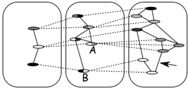
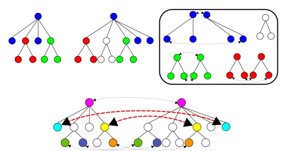
Figure 1. Example of a M iGaL structure of size three defined by three graphs and two refinements.
2.1. Definition
From now on, we adopt the following notations. Given a set S, we denote by |S| its cardinality. Let G(V, E) be a graph with vertex set V (G) = {v1, . . . , v|V (G)|} and edge set
E(G) = {e1, . . . , e|E(G)|}.
We start by defining the new data structure. It can be described as a layered sequence of graphs, with each graph linked to its neighbours by two applications, one of which corresponds to an abstraction from the previous graph, the other to a refinement leading to the next graph. The formal definition of the MultIGrAphLayers data structure is as follows.
Definition 1 (Definition of a M iGaL) A M iGaL structure M (G, R) of size |M | is defined as a layered sequence G = G1, . . . , G|M| of |M | graphs and a sequence R = α1, . . . , α|M|−1
of |M | − 1 applications called refinements. Each refinement αi is an application from V (Gi)
to P(V (Gi+1)), that is, each vertex in V (Gi) has a subset of V (Gi+1) as image. The inverse
application of αi, denoted by βi, is a surjection called an abstraction that maps every vertex
in V (Gi+1) to a vertex of V (Gi). In addition, M (G, R) satisfies the following two conditions:
1. For each vertex v ∈ V (Gi), the subgraph induced by αi(v) is connected and not empty.
2. For each edge (u, v) ∈ E(Gi), there exists at least one vertex of αi(u) connected to a
vertex of αi(v).
Figure 1illustrates this definition. From now on, we refer to the first graph of a MiGaL as the top graph and to the last one as the bottom graph. Note that there are no restrictions on the type of graphs that define a MiGaL structure. The comparison algorithm we provide later is therefore as general as possible.
This structure is clearly useful to encode data at different levels of detail. A comparable data structure called a Hierarchical Graph (denoted by H-Graph) has been used in [7, 8, 21, 11] to represent the environment (towns, buildings, rooms, . . . ) and drive robots in space. Godin et al. in [13, 9] use a similar structure, that they call quotiented trees, to model and study plants. Compared to the latter, MiGaLs can represent graphs and not just trees. Contrary to H-Graphs, MiGaLs can, in a given layer, connect vertices that are linked, through the abstraction function β, to vertices that are unconnected in an upper layer. This is illustrated
in Figure 1 by the arrow in layer 3 that links two vertices which correspond in layer 2 to the (abstracted) vertices A and B that are unconnected. This property of MiGaLs is justified later in the context of RNA secondary structures where it allows to take into account so-called pseudo-knots. MiGaLs and H-Graphs differ also in that, in MiGaL, each vertex (except in the last layer) necessarily has an image by the refinement and is itself (unless it is part of the first layer), by abstraction, the image of a vertex. This is not required in H-Graphs. MiGaLs is therefore neither a generalisation nor a special case of H-Graphs. The two structures are different. Although MiGaLs, and doubtless H-Graphs, can have many applications, the MiGaL structure is particularly adapted to comparing RNAs.
2.2. Top-Down comparison algorithm
In this section, we present an algorithm to compare two MiGaLs. The algorithm performs a top-down traversal of the structure. We assume both MiGaLs have the same number of layers, and compare them layer by layer starting with the graph at the top. The result of the comparison at a given layer is transmitted to the next layer by colouring vertices and edges of the graph and using the refinement application. We then compare the two graphs of the next layer taking into account such colouring. The process continues until the last layer is reached (bottom graph).
This approach assumes the existence of an algorithm allowing to compare two graphs of a same layer. This algorithm clearly depends on the data that is modelled using a MiGaL. In what follows, we consider a black box that is able to produce an extended mapping between two graphs where by an extended mapping is meant the following:
Definition 2 (Extended mapping) Given two graphs G1 and G2, we define an
extended mapping M between them as a set of couples of vertex sets of the two graphs: M= {(S1, S2)|S1⊂ V (G1) and S2⊂ V (G2)} such that for all (S1, S2), (S1′, S2′) ∈ M:
• S1 is a connected component of G1
• S2 is a connected component of G2
• (S1, S2) = (S′1, S2′) or S1∩ S1′ = ∅ and S2∩ S2′ = ∅
We define a colour-partitioned graph G with vertex set V (G) as a graph fitted with an application CG : S ⊂ V (G) → N+ which gives a colour to each vertex of S ⊂ V (G) such that
subgraphs defined by vertices of the same colour are connected. For convenience, uncoloured vertices are given the colour 0. The vertices with colour 0 are therefore elements of V (G) \ S. We now extend the definition of an extended mapping to colour-partitioned graphs as follows. Definition 3 (Colour-constrained extended mapping) Given two colour-partitioned graphs G1 and G2, a colour constrained extended mapping M between them is defined as an
extended mapping which further satisfies the following conditions:
• ∀(S1, S2) ∈ M, every vertex of S1 has the same colour c and every vertex of S2also has
this colour c.
• There is no vertex of G1 or G2 coloured with 0 that is involved in M.
Now that we have defined a mapping on colour-partitioned graphs, we give a general algorithm for comparing two MiGaLs, M (G, R) and M′(G′, R′), having the same number
Compare(M (G, R), M′(G′, R′))
1. colour= 2
2. Set all vertices of G1 and G′1 to 1.
3. for each layer i from 1 to |M |
4. M= B(Gi, G′i)
5. set the color of V (Gi+1) and V′(G′i+1) to 0
6. for each couple of sets (u, v) in M
7. for all nodes n in u
8. set the colour of nodes in α(n) to colour
9. for all nodes m in v
10. set the colour of nodes in α′(m) to colour
11. set colour to colour + 1
12. return M1...|M |
Figure 2. Algorithm for the comparison of two MiGaL structures using an external algorithm B that computes a colour-constrained mapping between two colour-partitioned graphs.
of layers. This number is denoted by |M | = |M′|. The algorithm assumes again that we have a black box B that computes a colour-constrained mapping between two colour-partitioned graphs.
The initialisation step colours the vertices of G1 and G′1 with 1.
The algorithm is then divided into |M | steps. For each layer i from 1 to |M |, we compute the mapping Mi between Gi and G′i using B and (except for the last step) colour the vertices of
Gi+1and G′i+1such that vertices associated by the mapping have the same colour and vertices
absent from Mi are coloured with 0. The result of the algorithm is the set of all mappings
between each pair of layers.
The pseudo-code of this algorithm is shown in Figure 2. Let b be the time complexity of algorithm B; the time required to compare two MiGaLs of size n is O(n ∗ b ∗ |V (Gn)|).
It is important to notice that the main idea of this algorithm is to compute mappings from the top to the bottom layer. Each layer is compared using the mapping of the previous one without reconsidering the choices implied by this mapping.
We now present a practical application of the MiGaL structure and of the comparison algorithm to the study of RNA secondary structures. In particular, we show how to significantly improve the runtime of algorithm B by taking advantage of the node-colouring.
3. RNA-MiGaL
RNAs are one of the most important molecules in a cell. They are composed by a succession of nucleotides, also called bases and denoted by A, C, G and U. Inside a cell, RNAs do not keep a linear form but instead fold in space. The fold is given by the set of interactions between
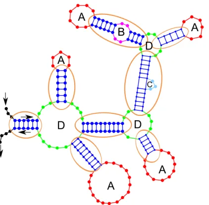
Figure 3. RNA Secondary Structure: the dots represent the nucleotides (bases) of the RNA. Helices correspond to consecutive base pairs, hairpin-loops are indicated by A, internal-loops by B,
bulges by C and multi-loops by D. Stems are surrounded.
nucleotides. An RNA can be described at three different levels, respectively called its primary, secondary and tertiary structures. The primary structure refers to the sequence of nucleotides. The secondary structure is composed of the list of base pairs that participate in a helix (see below). The tertiary structure corresponds to all interactions (base pairings) in the RNA, that is, to its fold in space.
The function of an RNA (be it the well known ribosomal and transfert RNAs or the more recently discovered snoRNAs, microRNAs, etc.) is strongly linked to the shape adopted by the RNA in space. It is generally accepted that two RNAs that have the same function will often have closely similar secondary structures but not necessarily similar primary structures. Considering this, it is fundamental to have efficient algorithms to compare RNAs from the point of view of their secondary structures.
Various structural elements can be distinguished in the secondary structure of an RNA (see Figure 3): helices which correspond to consecutive base pairs, hairpin-loops which are
Figure 4. Example of pseudo-knot (picture from wikipedia)
unpaired bases at the end of an helix, internal-loops defined by the unpaired bases between two helices and called bulges when one side is empty, multi-loops which are the meeting point of at least three helices and, finally, stems that are series of helices, internal-loops and bulges. Another element comsidered by some as being part of the secondary structure of an RNA, and by other authors as part of its tertiary structure, is the so-called pseudo-knot (see Figure 4). A pseudoknot is a structural element containing two stem-loop structures in which the first stem’s loop forms part of the second stem. In this paper, we do not take pseudo-knots into account.
Many approaches have been used for modelling secondary structures. Mainly, three codings have been proposed to represent RNA secondary structures: rooted ordered trees [26]; arc annotated sequences [5]; 2-intervals [24].
Since our purpose in this paper is to illustrate the interest of using a multiple layer model for RNAs, we focus on tree models. We thus represent secondary structures by rooted ordered trees. The root corresponds to the beginning and the end of the molecule. The order between the children of a node corresponds to the orientation of the sequence. In fact, we can use different tree models depending on the information we want to encode. In [26], Zuker and Sankoff use trees where internal nodes code for base pairs and leaves code for free nucleotides. This tree can be compacted [10] into a homeomorphically irreductible tree where internal nodes correspond to helices and leaves correspond to fragments of unpaired bases. Shapiro in [22] uses a tree where edges code for helices and nodes are labelled on {M, B, I, H, R} (multi-loop, budge, internal-loop, hairpin-loop and the root). We can also use a more abstract tree where edges code for stems and nodes for multi-loops and hairpin-loops, or just for multi-loops.
To compare rooted ordered trees, there exist essentially two methods. The first is edit distance [23] based on three edit operations. A substitution changes the label of a node. A deletion removes a node of the tree, its children are then re-attached to the node’s father preserving the relative order between nodes. An insertion is the opposite operation of a deletion. If we assign a score to each of these operations, we can define the edit distance between two trees as the minimum of the score of a series of edit operations (sum of the score
Figure 5. Classical edit distance vs edit distance with fusions on rooted ordered labelled (on nodes and edges) trees. In the first line, the tree A is edited by the edge fusion of a − 3 with ba − 1. Then the node 6 is split with a node split operation and node 2 is changed into 1. The second line shows how to edit A into B with the classical edit distance. First, c − 3 and a − 3 are deleted and ba − 1 is
substituted by aba − 1. Then, node b − 2 is inserted and 6 and 2 are substituted by 4 and 1.
of each operation) that transforms the first tree into the second one. Recently, Allali et al. [1] extended this distance by introducing four new operations: node fusion, edge fusion and the opposite operations of node split and edge split. These operations allow to address some of the limitations of the classical edit distance when comparing RNA secondary structures using high level trees (where nodes and edges code for secondary structure elements, not for nucleotides). The complexity of the classical edit distance algorithm provided by Zhang and Shasha [25] is O(|T |∗min(leaf (T ), height(T ))∗|T′|∗min(leaf (T′), height(T′))) where leaf (T ) is the number
of leaves in the tree T and height(T ) is its height. In the worst case (fan tree), the complexity is in O(|T |2∗ |T′|2). In [17], Klein gave an O(n3log n) algorithm to compute this distance
where n is the size of the trees. The complexity of the edit distance with fusion operations [1] is O((2d)l∗ |T | ∗ min(leaf (T ), height(T )) ∗ (2d′)l∗ |T′| ∗ min(leaf (T′), height(T′))) where d
is the degree of T and l the maximum number of consecutive fusions per node.
The second method for comparing rooted ordered trees is by performing a tree alignment [15, 16]. In this case, the goal is to insert blank labelled nodes in the two trees such that they become isomorphic. The score of the alignment corresponds to the sum of the scores of the association of node labels (the blank character assumes the role of an insertion or a deletion in a sequence alignment). The optimal score, maximal or minimal depending on the scoring scheme adopted, is then sought. A tree alignment can be expressed as an edit distance
We now suggest a new modelling of RNA secondary structures based on the MiGaL data structure introduced earlier in the paper. We thus call RNA-MiGaL a MiGaL structure composed by four layers, each modelled by a rooted ordered and labelled tree. In [12, 20], Giegerich et al. introduced the concept of the abstract shapes of an RNA secondary structure that is related to our layers. Their shapes however are less detailed, the general structure of the elements only is preserved, and any information of size is discarded.
The next section is dedicated to a description of RNA-MiGaL. 3.1. The four layers definition
The four layers contained in an RNA-MiGaL correspond to the secondary structure of an RNA observed at different levels of detail. Thus, each layer is modelled by a rooted ordered labelled tree. In the bottom layer, nodes and leaves code for nucleotides while the top layer encodes the network of multi-loops of an RNA. This choice has been dictated by two assumptions. The first, already mentioned, is that structure is more important than sequence. Thus we introduce information concerning the nucleotide sequence at the bottom layer only. This is the layer that will be treated last by the comparison algorithm. The second is that the network of multi-loops can be considered as the skeleton of the secondary structure of an RNA. RNAs of the same family should thus have strongly conserved multi-loop networks. For this reason, the top layer of an RNA-MiGaL is a tree that codes for the multi-loop network. Intermediate layers correspond to the structure encoded using stems or helices.
We provide below a summary of the layers and of the meaning of a node and a leaf in each layer:
• The tree of layer 1 corresponds to the multi-loop network. The nodes encode multi-loops and the edges encode stems. In the nodes, we store the number of helices connected by the multi-loop. In the edges, we store the number of nucleotides contained in the stem. • Layer 2 consists in the structure defined by the stems. The internal nodes represent
multi-loops, leaves represent hairpin-loops and edges encode stems. In the edges, we store the number of base pairs and the number of unpaired bases contained in the stem. In the internal nodes and leaves, we store the number of unpaired bases contained in the multi-loops and hairpin-loops.
• The tree of layer 3 encodes secondary structure elements: nodes encode hairpin-loops, multi-loops, internal-loops and bulges and store the number of unpaired bases of the corresponding element. The edges represent helices and store the number of base pairs of the helices.
• The last tree models the RNA primary structure. The internal nodes thus represent base pairs and leaves unpaired bases. Both store the names of the corresponding bases. All the numerical values stored in the nodes and edges of the first three layers are floating numbers.
The abstractions β0,1,2of the MiGaL model encode the natural inclusion between structural
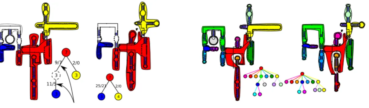
Figure 6. Result of the comparison of two Group I Introns. On the left, the result of the comparison of the trees of layer 1; on the right, the result of the comparison of the trees of layer 2.
Abstraction β1maps helices, internal loops and bulges to the stems of layer 1, while multi-loops
and hairpin-loops are mapped to their corresponding loops in layer 1. Finally, abstraction β0
associates the multi-loops and connected stem-hairpin-loops of layer 1 to the multi-loops of layer 0, while the stems between two multi-loops in layer 1 are mapped to a same stem of layer 0.
3.2. RNA-MiGaL comparison
The problem now is to compare two secondary structures using RNA-MiGaLs. To do so, we use edit distance with fusions and the algorithm described in [1] to compare the pairs of trees of layers 1, 2 and 3. To take into account the colour of the nodes and edges, we just have to test if two nodes or edges have the same colour to allow them to be fusioned (in a tree) or substituted (between the trees). The trees of layer 4 are compared using the classical edit distance (no fusions). Similarly, only nodes of a same colour in layer 4 can be mapped to each other. It may be interesting in the future to have operations which allow to pair two unpaired bases, or to separate a base pair into two unpaired bases. Such operations have been defined in [18] but Blin et al. proved in [2] that the computation of the edit distance between two trees allowing for these operations is NP-Complete.
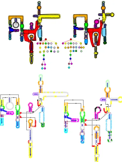
Figures6and7show the result of the comparison using RNA-MiGaLs between two Group I Intron RNAs retrieved from [4]. The left RNA is found in Acanthamoeba griffini and the right one in Chlorella sorokiniana.
The time complexity required to compare two trees of a same layer is O((2d)ln4) for the
first 3 layers and O(n4) for the last layer with n being the size of the trees. Since we colour
nodes while we progress in the comparison, and, once trees are coloured, substitutions and fusions can only be performed on nodes of same colour, we may wonder if it is not possible to compare separately the subtrees defined by each colour.
Figure 7. Result of the comparison of two Group I Introns. On the top, the comparison of the trees of layer 3; on the bottom, the result of the comparison of the trees of layer 4.
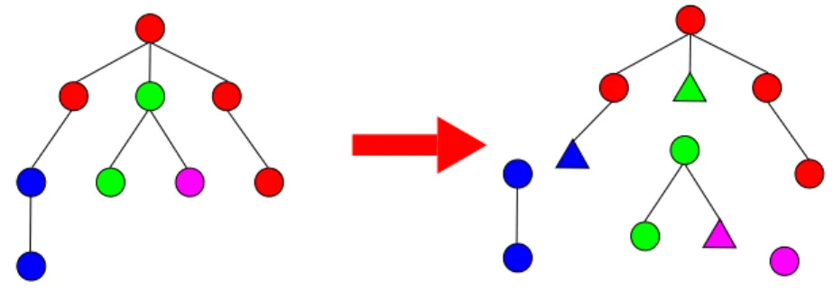
Figure 8. Potential problem when splitting a tree according to colour to optimise an edit computation.
The response is positive but it requires some attention as is shown in the following example. Figure8presents on the top left a colour-partitioned tree, with white corresponding to colour 0. In the box, we have split each tree into subtrees according to their colour and computed the edit distance between these trees separately. The nodes associated by the mapping are linked by dashed lines. We have then reported the result of the computations on the original trees. The problem is pointed to by the bold dashed lines in the tree at the bottom. We have two couples of nodes associated via two different computations. Inside each computation, the relative order of the nodes is respected by the edition (we work on ordered trees). However, in the final tree, the associations do not respect the order between the nodes.
We therefore have to modify the algorithm to take into account the presence of a subtree of a given colour x hanging from an edge of a subtree of colour y 6= x. To do so, we introduce anchors during the splitting step. When we split trees into subtrees according to their colour, we add anchors to the subtrees. These anchors represent the subtrees of another colour that hang from an edge of the subtree being considered as shown in Figure9. The anchors have the same colour as the subtrees they stand for. We then have to modify the edit distance scoring scheme such that:
• deleting the anchor of colour c costs the deletion of the subtree corresponding to the anchor;
• an anchor of colour c can only match with an anchor of the same colour.
Finally, we order the edit computations according to the dependence implied by the colouring scheme, that is, we consider the subtree from the leaves to the root.
Figure 9. Splitting the left tree into subtrees according to the colours of the nodes and the addition of anchors (represented by triangles).
We can now rewrite the time and space complexity required to compare two trees of a given layer as the sum of the time required to compare each subtree. In the extreme, if we split the trees of size n into n subtrees of one node, then the time required to compare the trees becomes linear!
In the worst-case, the time complexity is still 0((2d)l× n4) for each level but in the case of
RNAs, on average, the tree at each layer contains a number of subtrees that is proportional to the size of the tree, and the observed time complexity is close to linear except for the first layer.
3.3. Experimental results
We implemented the algorithm for comparing two RNA secondary structures inside a package called MiGaL which runs on the GNU/Linux platform. It is available for download at http://igm.univ-mlv.fr/˜allali/. The code is written in C++. We provide in this section three series of tests done on a PC with a single 1.6GHz processor Intel Pentium M with 1Gb of RAM memory under Debian GNU/Linux. Three series of tests were performed. They are described in what follows.
3.3.1. Time to compare two RNA secondary structures
The first series of tests we ran aimed at evaluating the time required to compare two RNA secondary structures on four different data sets. Figure10shows the results observed with two algorithms. The first is the classical Zhang and Shasha algorithm [25], that we denote by zs, applied to the bottom tree of rna-migal. The second, denoted by rna-migal, is our comparison algorithm with anchors optimisation. Both algorithms were applied using cost functions defined on reals (that is, on float numbers).
It is important to observe that, since the same algorithm is used to compare different trees given as input, each one having also different kinds of nodes, there may be some time lost
RNAs Size zs rna-migal RNAseP (21) 345.4 0.48 / 1.26 / 0.78 0.05 / 0.12 / 0.07 GroupI (36) 541.7 0.68 / 4.65 / 1.62 0.1 / 0.67 / 0.22 16S (91) 1744.8 36.25 / 128.1 / 62.93 0.34 / 0.94 / 0.51
23S (15) 2721.52 - 6.23 / 321.63 / 107.85
Figure 10. Computation time for comparing different kinds of RNA secondary structures using two algorithms. The first algorithm (zs) is the classical edit distance between two RNAs using Zhang and Shasha’s [25] algorithm on the tree corresponding to the bottom layer of RNA-MiGaL. The second (rna-migal) is the algorithm for comparing two MiGaLs using the anchors optimisation. The times indicated for the two algorithms are, respectively, the minimum/maximum/average times in seconds. In the case of our method, the times shown (without and with anchors optimisation) take into account the time required for loading the RNAs and for building the corresponding MiGaL structures. The number of comparisons used to obtain these execution times appears in parenthesis in the first column.
because of genericity. Indeed, it is possible to improve the performance of the Zhang and Shasha’s algorithm by using constant cost functions and a dedicated implementation. In the same way, it is possible to improve our RNA-MiGaL algorithm by using a specific source code for each layer.
The first row of Figure10results from the 21 pairwise comparisons made on seven RNAsePs extracted from the RNAseP database [3]. Such RNAs are small, around 350 nucleotides. Their multi-loop networks are quite simple. The top layer tree corresponds therefore to very small trees, having from three to six nodes with a degree bounded by one (the trees are in fact paths).
As second example (second row), we considered nine Group I introns from the Comparative RNA database[4] to which we applied all possible pairwise comparisons. The smallest Group I intron has 430 nucleotides, the longest, which contains a long unfolded part of 420 nucleotides, has 1032 nucleotides. The multi-loop networks of such RNAs lead to trees of 4-5 nodes with a degree bounded by two.
The results in the third row of Figure10come from the comparison of fourteen 16S-RNAs extracted also from the Comparative RNA database. Their lengths range from 1496 to 2291 nucleotides. The multi-loop networks are bigger than for the two previous examples. They correspond to trees of 19 nodes with a degree bounded by two.
Finally, the last row of Figure 10 shows the results of the comparison of six 23S-RNAs which come again from the Comparative RNA database. Their lengths go from 2928 to 3555 nucleotides. Such RNAs contain from 47 to 73 multi-loops. The top layer trees have therefore between 47 and 73 nodes with a degree bounded by 11. In this case, we were not able to use zs as the computations led to a stack overflow. Indeed, the top layer contains less than one hundred nodes which is manageable by our edit-distance-with-fusions algorithm while the bottom layer contains more than two thousand nodes which is hardly manageable by an O(n4)
algorithm.
As we can see, rna-migal is very performing and allows to compare large RNAs in a short time thanks to the colouring scheme and the tree splitting optimisation. In fact, the time
P.aby S.aci B.sub T.mar H.sap M.mus O.sat Z.may P.aby 0 137.5 315.5 275.5 665 669 601 612.75 S.aci 137.5 0 314 299.5 656.75 656.5 590 602 B.sub 315.5 314 0 157 717.5 728.5 693.25 693.5 T.mar 275.5 299.5 157 0 721 731.5 692.75 680.75 H.sap 665 656.75 717.5 721 0 69.25 267 287.75 M.mus 669 656.5 728.5 731.5 69.25 0 236.25 259.25 O.sat 601 590 693.25 692.75 267 236.25 0 32.25 Z.may 612.75 602 693.5 680.75 287.75 259.25 32.25 0
Abbreviation Name Phylogenetic
Level 1 Level 2 Level 3 P.aby Pyrococcus abyssi Archaea Euryarchaeota Thermococci S.aci Sulfolobus acidocaldarius Archaea Crenarchaeota Thermoprotei B.sub Bacillus subtilis Bacteria Firmicutes Bacilli T.mar Thermotoga maritima Bacteria Thermotogae Thermotogae H.sap Homo sapiens Eukaryota Metazoa Mammalia M.mus Mus musculus Eukaryota Metazoa Mammalia O.sat Oryza sativa Eukaryota Viridiplantae Tracheophyta Z.may Zea mays Eukaryota Viridiplantae Tracheophyta
Figure 11. Scoring matrix for 8 16S-RNAs extracted from The comparative RNA database [4]. For each row, we put in bold the best value (the smallest one).
required by rna-migal to compare two RNAs is roughly the same as the time required to compare the first layers of the MiGaL structures. The time complexity of the edit-distance-with-fusions algorithm depends strongly on the degree of the input trees. This explains why it takes so long to compare the 23S-RNAs in relation to the other RNAs: the huge central multi-loop with many branching helices leads to a high node degree in the top layer tree. 3.3.2. Using MiGaL to build phylogenetic trees
The second test we performed consisted in comparing eight of the 14 16S-RNAs from the Comparative RNA database and in using the scores of the edit computations on the bottom layers of the MiGaL structures to build a phylogenetic tree using the neighbour joining algorithm implementation of quicktree [14]. For the purposes of the illustration, two RNAs only were chosen for each of the four main evolutionary groups present in the data, archea, bacteria, mammals and plants. The remaining 6 RNAs were well classified by the method
S.acidocal P.abyssi.x T.maritima B.subtilis Z.mays.xml O.sativa.x M.musculus H.sapiens. S.acidocal P.abyssi.x T.maritima B.subtilis Z.mays.xml O.sativa.x M.musculus H.sapiens.
Figure 12. Result of the application of quicktree[14] to compute the tree corresponding to the matrix given in Figure11(neighbour-joining method). Trees were drawn with the drawtree PHYLIP program
[6], the left one is without edge length.
P.aby S.aci B.sub T.mar H.sap M.mus O.sat Z.may
P.aby 0.0 137.5 259.2 243.5 623.2 630.2 574.0 577.5 S.aci 137.5 0.0 276.5 269.8 617.0 619.2 563.5 565.5 B.sub 259.2 276.5 0.0 147.8 673.0 679.0 633.0 632.2 T.mar 243.5 269.8 147.8 0.0 670.0 679.0 632.2 631.5 H.sap 623.2 617.0 673.0 670.0 0.0 69.2 250.8 260.2 M.mus 630.2 619.2 679.0 679.0 69.2 0.0 223.5 236.2 O.sat 574.0 563.5 633.0 632.2 250.8 223.5 0.0 32.2 Z.may 577.5 565.5 632.2 631.5 260.2 236.2 32.2 0.0
Figure 13. Distance matrix using the classical edit distance of Zhang and Shasha. Observe that the distance computed with a classical edit distance leads to values that are smaller or equal to the ones computed with rna-migal. Indeed, rna-migal is a restricted version of a classical edit distance because
indicates that plants, mammals, bacteria and archea are correctly grouped together. This test is, of course, preliminary. We are currently applying our method to infer phylogenetic trees for closely related species as such represent a better test of the accuracy of RNA-MiGaL. Indeed, in this case using the sequences often leads to wrong results.
The matrix in Figure13shows the scores obtained by the classical edit distance algorithm of Zhang and Shasha applied to the same eight 16S-RNAs. The scoring scheme used to compute the distances is also exactly the same as the one used to compute the matrix in Figure11. The differences between the two sets of scores result therefore only from the constraint of locality (colour) brought from the upper layers of the MiGaL structure to the bottom one. The values z in the matrix obtained with the classical edit distance are distant from the corresponding ones, denoted by m, obtained with rna-migal by at most 10% in all cases (that is, m ≤ 1.1 ∗ z) except five where the distance is between 10 and 15% (4 of the 5 cases), or is of 21% (last case). The resulting trees are isomorphic. The new rna-migal approach leads therefore in this case to essentially equivalent results in a much faster way.
3.3.3. Addressing the scattering effect problem
The last test we show gives an example where rna-migal can significantly improve the results of the comparison.
For this test, we ran zs and rna-migal on the RNAs used as illustrations in [1]. In this paper, the authors point out a common problem when comparing RNA secondary structures using previous methods, the so-called scattering effect. This problem corresponds to base pairs that are mapped to one another (through a substitution of their labels) although they belong to structurally unrelated regions. In Figure 14, we surrounded two such wrong substitutions. These two wrong mappings are chosen by a classical edit distance algorithm because they cost less than performing deletions. The result with rna-migal is shown in Figure 15. We surrounded the regions affected by the constraint of locality brought by the first-to-last layer comparison. We can see that the previous wrong mapping can not be made anymore because the corresponding bases do not belong to the same secondary structure elements.
4. Conclusion
We introduced in this paper a new data structure and an algorithm for comparing such structures. Both are generic and may be applied to very different types of problems. They are particularly interesting for comparing objects that may be described at different levels of abstraction.
RNA secondary structures are one example of such objects and we therefore showed how to optimise the generic algorithm, in particular its special colouring scheme for going from one level of abstraction to the next, to compare two RNA secondary structures. The results obtained are very satisfying. In particular, the algorithm addresses the so-called scattering effect described in the literature [1]. The new algorithm allows to compare large sized structures
Figure 14. Result of the comparison of two RNAseP (of Streptococcus gordonii (left) and Thermotoga maritima) extracted from [3] using the classical edit distance of Zhang and Shasha. An example of
scattering effect corresponds to the surrounded substitutions.
Figure 15. Result of the comparison of the RNAs of Figure 14 using rna-migal. The effect of the constraints of locality brought by the first-to-last layer comparisons are shown by the surrounded
The current implementation of rna-migal does not allow to deal with pseudo-knots. We plan to introduce this possibility at the second layer from the top. Pseudo-knots correspond to edges between two secondary structure elements. Adding such nodes is possible because we allow the introduction of an edge between nodes of which the abstractions in the upper layer are unconnected. The fact that pseudo-knots are not considered yet in rna-migal is therefore a limitation of the current implementation, not of the MiGaL structure.
Algorithms working with hierarchical structures in general often consider as part of the algorithm to optimise the number of levels in the hierarchy instead of working with a fixed number as is done in rna-migal. In the case of RNAs, we are not sure optimising the number of levels would lead to a biologically realistic model. This could, however, be worth checking. The number of levels considered may also be questioned. For example, in [19], the authors used a hierarchy with two layers only, which correspond to our two last. In particular, it might be interesting to explore what happens with a model that skips the first layer.
Acknowledgements
We would like to thank Claude Thermes and Yves d’Aubenton-Carafa for their help all along the development of MiGaL.
REFERENCES
1. J. Allali and M.-F. Sagot. A new distance for high level rna secondary structure comparison. IEEE/ACM Trans. Comput. Biol. Bioinformatics, 2(1):3–14, 2005.
2. G. Blin, G. Fertin, I. Rusu, and C. Sinoquet. RNA sequences and the edit(nested,nested) problem. Technical Report RR-IRIN-03.07, LINA, Universit´e de Nantes, 2003.
3. J. W. Brown. The ribonuclease p database. Nucleic Acids Research, 24(1):314, 1999.
4. J. J. Cannone, S. Subramanian, M. N. Schnare, J. R. Collett, L. M. D’Souza, Y. Du, B. Feng, N. Lin, L. V. Madabusi, K. M. Muller, N. Pande, Z. Shang, N. Yu, and R. R. Gutell. The comparative RNA web (CRW) site: an online database of comparative sequence and structure information for ribosomal, intron, and other RNAs. BMC Bioinformatics, 3(1), 2002.
5. P. A. Evans. Finding common subsequence with arcs and pseudoknots. In Proceedings of the 10th Annual Symposium on Combinatorial Pattern Matching (CPM’99), number 1645 in LNCS, pages 270–280, 1999. 6. J. Felsenstein. Phylip (phylogeny inference package) version 3.6. distributed by the author., 2005. 7. J.-A. Fernandez and J. Gonzalez. Hierarchical graph search for mobile robot path planning. In ICRA,
pages 656–661, 1998.
8. J.-A. Fern´andez-Madrigal and J. Gonz´alez. Multihierarchical graph search. IEEE Trans. Pattern Anal. Mach. Intell., 24(1):103–113, 2002.
9. P. Ferraro and C. Godin. An edit distance between quotiented trees. Algorithmica, 36:1–39, 2003. 10. W. Fontana, D. A. M. Konings, P. F. Stadler, and P. Schuster. Statistics of RNA secondary structures.
Biopolymers, 33:1389–1404, 1993.
11. C. Galindo, J.-A. Fern´andez-Madrigal, and J. Gonz´alez. Improving efficiency in mobile robot task planning through world abstraction. IEEE Transactions on Robotics, 20(4):677–690, 2004.
12. R. Giegerich, B. Voß, and M. Rehmsmeier. Abstract shapes of RNA. Nucleic Acids Research, 32(16):4843– 4851, October 15 2004.
13. C. Godin and Y. Caraglio. A multiscale model of plant topological structures. Journal of theoretical biology, 191:1–46, 1998.
14. K. L. Howe, A. Bateman, and R. Durbin. Quicktree: building huge neighbour-joining trees of protein sequences. Bioinformatics, 18(11):1546–1547, 2002.
15. M. H¨ochsmann, T. T¨oller, R. Giegerich, and S. Kurtz. Local similarity in RNA secondary structures. In Proceedings of the IEEE Computer Society Conference on Bioinformatics, page 159. IEEE Computer Society, 2003.
16. T. Jiang, L. Wang, and K. Zhang. Alignment of trees - an alternative to tree edit. In Proceedings of the 5th Annual Symposium on Combinatorial Pattern Matching, pages 75–86. Springer-Verlag, 1994. 17. P. N. Klein. Computing the edit-distance between unrooted ordered trees. In Proceedings of the 6th
Annual European Symposium on Algorithms, pages 91–102. Springer-Verlag, 1998.
18. G. Lin, B. Ma, and K. Zhang. Edit distance between two RNA structures. In RECOMB, pages 211–220, 2001.
19. A. Ouangraoua, P. Ferraro, L. Tichit, and S. Dulucq. Local similarity between quotiented ordered trees. Journal of Discrete Algorithms, article in press, available on line 12 May 2006.
20. J. Reeder and R. Giegerich. Consensus shapes: an alternative to the sankoff algorithm for RNA consensus structure prediction. Bioinformatics, 21(17):3516–3523, August 22 2005.
21. E. Remolina, J. A. Fernandez, B. Kuipers, and J. Gonzalez. Formalizing regions in the spatial semantic hierarchy: An AH-graphs implementation approach. Lecture Notes in Computer Science, 1661:109–124, 1999.
22. B. Shapiro. An algorithm for multiple RNA secondary structures. Comput. Appl. Biosci., 4(3):387–393, 1988.
23. K.-C. Tai. The tree-to-tree correction problem. J. ACM, 26(3):422–433, 1979.
24. S. Vialette. Pattern matching problems over 2-interval sets. In Proceedings of the 13th Annual Symposium on Combinatorial Pattern Matching, pages 53–63. Springer-Verlag, 2002.
25. K. Zhang and D. Shasha. Simple fast algorithms for the editing distance between trees and related problems. SIAM J. Comput., 18(6):1245–1262, 1989.
26. M. Zuker and D. Sankoff. RNA secondary structures and their prediction. Bull. Math. Biol., 46:591–621, 1984.


![Figure 11. Scoring matrix for 8 16S-RNAs extracted from The comparative RNA database [4]](https://thumb-eu.123doks.com/thumbv2/123doknet/14430577.515106/16.892.203.692.312.448/figure-scoring-matrix-rnas-extracted-comparative-rna-database.webp)
