HAL Id: hal-01318486
https://hal.inria.fr/hal-01318486v4
Submitted on 5 Jan 2017
HAL is a multi-disciplinary open access
archive for the deposit and dissemination of
sci-entific research documents, whether they are
pub-lished or not. The documents may come from
teaching and research institutions in France or
abroad, or from public or private research centers.
L’archive ouverte pluridisciplinaire HAL, est
destinée au dépôt et à la diffusion de documents
scientifiques de niveau recherche, publiés ou non,
émanant des établissements d’enseignement et de
recherche français ou étrangers, des laboratoires
publics ou privés.
Neumann Decomposition
Michele Benzi, Bora Uçar
To cite this version:
Michele Benzi, Bora Uçar. Preconditioning Techniques Based on the Birkhoff–von Neumann
Decom-position. Computational Methods in Applied Mathematics, De Gruyter, 2016,
�10.1515/cmam-2016-0040�. �hal-01318486v4�
Research Article
Michele Benzi* and Bora Uçar
Preconditioning techniques based on the
Birkhoff–von Neumann decomposition
DOI: ..., Received ...; accepted ...
Abstract: We introduce a class of preconditioners for general sparse matrices
based on the Birkhoff–von Neumann decomposition of doubly stochastic ma-trices. These preconditioners are aimed primarily at solving challenging linear systems with highly unstructured and indefinite coefficient matrices. We present some theoretical results and numerical experiments on linear systems from a va-riety of applications.
Keywords: Preconditioning, parallel computing, doubly stochastic matrix,
bi-partite graphs, Birkhoff–von Neumann decomposition
MCS: 65F35, 65F08, 65F50, 65Y05, 15B51,05C70
Communicated by: Communicated by the editor.
1 Introduction
We consider the solution of linear systems 𝐴𝑥 = 𝑏 where 𝐴 = [𝑎𝑖𝑗] ∈ R𝑛×𝑛,
𝑏 is a given vector and 𝑥 is the unknown vector. Our aim is to develop and
investigate preconditioners for Krylov subspace methods for solving such linear systems, where 𝐴 is highly unstructured and indefinite.
For a given matrix 𝐴, we first preprocess it to get a doubly stochastic ma-trix (whose row and column sums are one). Then using this doubly stochastic matrix, we select some fraction of some of the nonzeros of 𝐴 to be included in the preconditioner. Our main tools are the well-known Birkhoff-von Neumann (BvN) decomposition (this will be discussed in Section 2 for completeness), and a splitting of the input matrix in the form 𝐴 = 𝑀 − 𝑁 based on its BvN de-composition. When such a splitting is defined, 𝑀−1 or solvers for 𝑀 𝑦 = 𝑧 are
*Corresponding Author: Michele Benzi: Department of Mathematics and Computer
Sci-ence, Emory University, Atlanta, USA. ([email protected]).
Bora Uçar: LIP, UMR5668 (CNRS - ENS Lyon - UCBL - Université de Lyon - INRIA),
required. We discuss sufficient conditions when such a splitting is convergent and discuss specialized solvers for 𝑀 𝑦 = 𝑧 when these conditions are met. We dis-cuss how to build preconditioners meeting the sufficiency conditions. In case the preconditioners become restrictive in practice, their LU decomposition can be used. Our motivation is that the preconditioner 𝑀−1can be applied to vectors via a number of highly concurrent steps, where the number of steps is controlled by the user. Therefore, the preconditioners (or the splittings) can be advan-tageous for use in many-core computing systems. In the context of splittings, the application of 𝑁 to vectors also enjoys the same property. These motiva-tions are shared by recent work on ILU preconditioners, where their fine-grained computation [9] and approximate application [2] are investigated for GPU-like systems.
The paper is organized as follows. We first give necessary background (Sec-tion 2) on doubly stochastic matrices and the BvN decomposi(Sec-tion. We then develop splittings for doubly stochastic matrices (Section 3), where we analyze convergence properties and discuss algorithms to construct the preconditioners. Later in the same Section, we discuss how the preconditioners can be used for arbitrary matrices by some preprocessing. Here our approach results in a gener-alization of the Birkhoff-von Neumann decomposition for matrices with positive and negative entries where the sum of the absolute values of the entries in any given row or column is one. This generalization could be of interest in other areas. Then, we give experimental results (Section 4) with nonnegative and also arbitrary matrices, and then conclude the paper.
2 Background and definitions
Here we define several properties of matrices: irreducible, full indecomposable, and doubly stochastic matrices.
An 𝑛 × 𝑛 matrix 𝐴 is reducible if there exists a permutation matrix 𝑃 such that 𝑃 𝐴𝑃𝑇 = [︂ 𝐴1,1 𝐴1,2 𝑂 𝐴2,2 ]︂ ,
where 𝐴1,1is an 𝑟 × 𝑟 submatrix, 𝐴2,2 is an (𝑛 − 𝑟) × (𝑛 − 𝑟) submatrix, and
1 ≤ 𝑟 < 𝑛. If such a permutation matrix does not exist, then 𝐴 is irreducible [25, Ch. 1]. When 𝐴 is reducible, either 𝐴1,1or 𝐴2,2 can be reducible as well, and
we can recursively identify their diagonal blocks, until all diagonal blocks are irreducible. That is, we can obtain
𝑃 𝐴𝑃𝑇 = ⎡ ⎢ ⎢ ⎢ ⎣ 𝐴1,1 𝐴1,2 · · · 𝐴1,𝑠 0 𝐴2,2 · · · 𝐴2,𝑠 .. . ... . .. ... 0 0 · · · 𝐴𝑠,𝑠 ⎤ ⎥ ⎥ ⎥ ⎦ ,
where each 𝐴𝑖,𝑖is square and irreducible. This block upper triangular form, with
square irreducible diagonal blocks is called Frobenius normal form [19, p. 532]. An 𝑛 × 𝑛 matrix 𝐴 is fully indecomposable if there exists a permutation matrix 𝑄 such that 𝐴𝑄 has a zero-free diagonal and is irreducible [7, Chs. 3 and 4]. If 𝐴 is not fully indecomposable, but nonsingular, it can be permuted into the block upper triangular form
𝑃 𝐴𝑄𝑇 = [︂ 𝐴1,1 𝐴1,2 𝑂 𝐴2,2 ]︂ ,
where each 𝐴𝑖,𝑖 is fully indecomposable or can be further permuted into the
block upper triangular form. If the coefficient matrix of a linear system is not fully indecomposable, the block upper triangular form should be obtained, and only the small systems with the diagonal blocks should be factored for simplicity and efficiency [12, Ch. 6]. We therefore assume without loss of generality that matrix 𝐴 is fully indecomposable.
An 𝑛 × 𝑛 matrix 𝐴 is doubly stochastic if 𝑎𝑖𝑗 ≥ 0 for all 𝑖, 𝑗 and 𝐴𝑒 =
𝐴𝑇𝑒 = 𝑒, where 𝑒 is the vector of all ones. This means that the row sums and
column sums are equal to one. If these sums are less than one, then the matrix
𝐴 is doubly substochastic. A doubly stochastic matrix is fully indecomposable
or is block diagonal where each block is fully indecomposable. By Birkhoff’s Theorem [4], there exist coefficients 𝛼1, 𝛼2, . . . , 𝛼𝑘 ∈ (0, 1) with∑︀𝑘𝑖=1𝛼𝑖 = 1,
and permutation matrices 𝑃1, 𝑃2, . . . , 𝑃𝑘 such that
𝐴 = 𝛼1𝑃1+ 𝛼2𝑃2+ · · · + 𝛼𝑘𝑃𝑘. (1)
Such a representation of 𝐴 as a convex combination of permutation matrices is known as a Birkhoff–von Neumann decomposition (BvN); in general, it is not unique. The Marcus–Ree Theorem states that there are BvN decompositions with 𝑘 ≤ 𝑛2− 2𝑛 + 2 for dense matrices; Brualdi and Gibson [6] and Brualdi [5] show that for a fully indecomposable sparse matrix with 𝜏 nonzeros, we have BvN decompositions with 𝑘 ≤ 𝜏 − 2𝑛 + 2.
An 𝑛×𝑛 nonnegative, fully indecomposable matrix 𝐴 can be uniquely scaled with two positive diagonal matrices 𝑅 and 𝐶 such that 𝑅𝐴𝐶 is doubly stochas-tic [24].
3 Splittings of doubly stochastic matrices
3.1 Definition and properties
Let 𝑏 ∈ R𝑛 be given and consider solving the linear system 𝐴𝑥 = 𝑏 where 𝐴 is doubly stochastic. Hereafter we assume that 𝐴 is invertible. After finding a representation of 𝐴 in the form (1), pick an integer 𝑟 between 1 and 𝑘 − 1 and split 𝐴 as
𝐴 = 𝑀 − 𝑁, (2)
where
𝑀 = 𝛼1𝑃1+ · · · + 𝛼𝑟𝑃𝑟, 𝑁 = −𝛼𝑟+1𝑃𝑟+1− · · · − 𝛼𝑘𝑃𝑘. (3)
Note that 𝑀 and −𝑁 are doubly substochastic matrices.
Definition 1. A splitting of the form (2) with 𝑀 and 𝑁 given by (3) is said to
be a doubly substochastic splitting.
Definition 2. A doubly substochastic splitting 𝐴 = 𝑀 − 𝑁 of a doubly stochastic
matrix 𝐴 is said to be standard if 𝑀 is invertible. We will call such a splitting an SDS splitting.
In general, it is not easy to guarantee that a given doubly substochastic splitting is standard, except for some trivial situation such as the case 𝑟 = 1, in which case 𝑀 is always invertible. We also have a characterization for invertible 𝑀 when 𝑟 = 2.
Theorem 1. Let 𝑀 = 𝛼1𝑃1+ 𝛼2𝑃2. Then, 𝑀 is invertible if (i) 𝛼1 ̸= 𝛼2, or
(ii) 𝛼1= 𝛼2 and all the fully indecomposable blocks of 𝑀 have an odd number
of rows (and columns). If any such block is of even order, 𝑀 is singular. Proof. We investigate the two cases separately.
Case (i): Without loss of generality assume that 𝛼1> 𝛼2. We have
𝑀 = 𝛼1𝑃1+ 𝛼2𝑃2= 𝑃1(𝛼1𝐼 + 𝛼2𝑃1𝑇𝑃2).
The matrix 𝛼1𝐼 + 𝛼2𝑃1𝑇𝑃2 is nonsingular. Indeed, its eigenvalues are of the
form 𝛼1+ 𝛼2𝜆𝑗, where 𝜆𝑗 is the generic eigenvalue of the (orthogonal, doubly
stochastic) matrix 𝑃𝑇
1 𝑃2, and since |𝜆𝑗| = 1 for all 𝑗 and 𝛼1 > 𝛼2, it follows
that 𝛼1+ 𝛼2𝜆𝑗̸= 0 for all 𝑗. Thus, 𝑀 is invertible.
Case (ii): This is a consequence of the Perron–Frobenius Theorem. To see
this, observe that we need to show that under the stated conditions the sum 𝑃1+
Since both 𝑃1 and 𝑃2 are permutation matrices, 𝑃1𝑇𝑃2 is also a permutation
matrix and the Frobenius normal form 𝑇 = Π(𝑃𝑇
1 𝑃2)Π𝑇 of 𝑃1𝑇𝑃2, i.e., the block
triangular matrix 𝑇 = ⎡ ⎢ ⎢ ⎢ ⎣ 𝑇1,1 𝑇1,2 · · · 𝑇1,𝑠 0 𝑇2,2 · · · 𝑇2,𝑠 .. . ... . .. ... 0 0 · · · 𝑇𝑠,𝑠 ⎤ ⎥ ⎥ ⎥ ⎦ , (4)
has 𝑇𝑖,𝑗 = 0 for 𝑖 ̸= 𝑗. The eigenvalues of 𝑃1𝑇𝑃2 are just the eigenvalues of
the diagonal blocks 𝑇𝑖,𝑖 of 𝑇 . Note that there may be only one such block,
corresponding to the case where 𝑃1𝑇𝑃2is irreducible. Each diagonal block 𝑇𝑖,𝑖is
also a permutation matrix. Thus, each 𝑇𝑖,𝑖is doubly stochastic, orthogonal, and
irreducible. Any matrix of this kind corresponds to a cyclic permutation and has its eigenvalues on the unit circle. If a block has size 𝑟 > 1, its eigenvalues are the 𝑝th roots of unity, 𝜀ℎ, ℎ = 0, 1, . . . , 𝑝 − 1, with 𝜀 = 𝑒2𝜋𝑖𝑝 , e.g., by the
Perron–Frobenius Theorem (see [17, page 53]). But 𝜆 = −1 is a 𝑝th root of unity if and only if 𝑝 is even. Since 𝑀 is a scalar multiple of 𝑃1+ 𝑃2= 𝑃1(𝐼 + 𝑃1𝑇𝑃2),
this concludes the proof.
Note that the fully indecomposable blocks of 𝑀 mentioned in the theorem are just connected components of its bipartite graph.
It is possible to generalize the condition (i) in the previous theorem as follows.
Theorem 2. A sufficient condition for 𝑀 =∑︀𝑟
𝑖=1𝛼𝑖𝑃𝑖 to be invertible is that
one of the 𝛼𝑖 with 1 ≤ 𝑖 ≤ 𝑟 be greater than the sum of the remaining ones.
Proof. Indeed, assuming (without loss of generality) that 𝛼1 > 𝛼2+ · · · + 𝛼𝑟,
we have
𝑀 = 𝛼1𝑃1+ 𝛼2𝑃2+ · · · + 𝛼𝑟𝑃𝑟
= 𝑃1(𝛼1𝐼 + 𝛼2𝑃1𝑇𝑃2+ · · · + 𝛼𝑟𝑃1𝑇𝑃𝑟).
This matrix is invertible if and only if the matrix 𝛼1𝐼 +∑︀
𝑟 𝑖=2𝛼𝑖𝑃
𝑇
1 𝑃𝑖is
invert-ible. Observing that the eigenvalues 𝜆𝑗 of∑︀𝑟𝑖=2𝛼𝑖𝑃1𝑇𝑃𝑖 satisfy
|𝜆𝑗| ≤ ‖𝛼2𝑃1𝑇𝑃2+ · · · + 𝛼𝑟𝑃1𝑇𝑃𝑟‖2≤
𝑟
∑︁
𝑖=2
𝛼𝑖< 𝛼1
(where we have used the triangle inequality and the fact that the 2-norm of an orthogonal matrix is one), it follows that 𝑀 is invertible.
Again, this condition is only a sufficient one. It is rather restrictive in practice.
3.2 Convergence conditions
Let 𝐴 = 𝑀 − 𝑁 be an SDS splitting of 𝐴 and consider the stationary iterative scheme
𝑥𝑘+1= 𝐻𝑥𝑘+ 𝑐, 𝐻 = 𝑀−1𝑁, 𝑐 = 𝑀−1𝑏 , (5) where 𝑘 = 0, 1, . . . and 𝑥0is arbitrary. As is well known, the scheme (5) converges to the solution of 𝐴𝑥 = 𝑏 for any 𝑥0 if and only if 𝜌(𝐻) < 1. Hence, we are
interested in conditions that guarantee that the spectral radius of the iteration matrix
𝐻 = 𝑀−1𝑁 = −(𝛼1𝑃1+ · · · + 𝛼𝑟𝑃𝑟)−1(𝛼𝑟+1𝑃𝑟+1+ · · · + 𝛼𝑘𝑃𝑘)
is strictly less than one. In general, this problem appears to be difficult. We have a necessary condition (Theorem 3), and a sufficient condition (Theorem 4) which is simple but restrictive.
Theorem 3. For the splitting 𝐴 = 𝑀 − 𝑁 with 𝑀 = ∑︀𝑟
𝑖=1𝛼𝑖𝑃𝑖 and 𝑁 =
−∑︀𝑘
𝑖=𝑟+1𝛼𝑖𝑃𝑖 to be convergent, it must hold that
∑︀𝑟
𝑖=1𝛼𝑖>
∑︀𝑘
𝑖=𝑟+1𝛼𝑖.
Proof. First, observe that since 𝑃𝑖𝑒 = 𝑒 for all 𝑖, both 𝑀 and 𝑁 have constant
row sums: 𝑀 𝑒 = 𝑟 ∑︁ 𝑖=1 𝛼𝑖𝑃𝑖𝑒 = 𝛽𝑒, 𝑁 𝑒 = − 𝑟 ∑︁ 𝑖=1 𝛼𝑖𝑃𝑖𝑒 = (𝛽 − 1)𝑒, with 𝛽 := ∑︀𝑟
𝑖=1𝛼𝑖 ∈ (0, 1). Next, observe that 𝑀
−1𝑁 𝑒 = 𝜆𝑒 is equivalent to
𝑁 𝑒 = 𝜆𝑀 𝑒 or, since we can assume that 𝜆 ̸= 0, to 𝑀 𝑒 = 1𝜆𝑁 𝑒. Substituting 𝛽𝑒
for 𝑀 𝑒 and (𝛽 − 1)𝑒 for 𝑁 𝑒 we find
𝛽𝑒 = 1
𝜆(𝛽 − 1)𝑒, or 𝜆 = 𝛽 − 1
𝛽 .
Hence, 𝛽−1𝛽 is an eigenvalue of 𝐻 = 𝑀−1𝑁 corresponding to the eigenvector 𝑒.
Since |𝜆| = 1−𝛽𝛽 , we conclude that 𝜌(𝐻) ≥ 1 for 𝛽 ∈ (0,12]. This concludes the proof.
Theorem 4. Suppose that one of the 𝛼𝑖appearing in 𝑀 is greater than the sum
of all the other 𝛼𝑖. Then 𝜌(𝑀−1𝑁 ) < 1 and the stationary iterative method (5)
Proof. Assuming (without loss of generality) that
𝛼1> 𝛼2+ · · · + 𝛼𝑘, (6)
(which, incidentally, ensures that the matrix 𝑀 is invertible) we show below that
‖𝐻‖2= ‖(𝛼1𝑃1+ · · · + 𝛼𝑟𝑃𝑟)−1(𝛼𝑟+1𝑃𝑟+1+ · · · + 𝛼𝑘𝑃𝑘)‖2< 1. (7)
This, together with the fact that 𝜌(𝐻) ≤ ‖𝐻‖2, ensures convergence. To prove
(7) we start by observing that
𝑀 = 𝛼1𝑃1+ · · · + 𝛼𝑟𝑃𝑟 = 𝛼1𝑃1 (︂ 𝐼 +𝛼2 𝛼1 𝑄2+ · · · + 𝛼𝑟 𝛼1 𝑄𝑟 )︂ ,
where 𝑄𝑖= 𝑃1𝑇𝑃𝑖. Thus, we have
𝑀−1= (𝛼1𝑃1+ · · · + 𝛼𝑟𝑃𝑟)−1=
1
𝛼1
(𝐼 − 𝐺)−1𝑃1𝑇 ,
where we have defined
𝐺 = − 1 𝛼1 𝑟 ∑︁ 𝑖=2 𝛼𝑖𝑄𝑖.
Next, we observe that ‖𝐺‖2< 1, since
‖𝐺‖2≤ 1 𝛼1 𝑟 ∑︁ 𝑖=2 𝛼𝑖‖𝑄𝑖‖2= 𝛼2+ · · · + 𝛼𝑟 𝛼1 < 1
as a consequence of (6). Hence, the expansion
(𝐼 − 𝐺)−1=
∞
∑︁
ℓ=0
𝐺ℓ
is convergent, and moreover
‖(𝐼 − 𝐺)−1𝑃1𝑇‖2= ‖(𝐼 − 𝐺)−1‖2≤ 1 1 − ‖𝐺‖2 ≤ 1 1 −(︁𝛼2 𝛼1 + · · · + 𝛼𝑟 𝛼1 )︁ .
The last inequality follows from the fact that ‖𝐺‖2≤∑︀𝑟𝑖=2 𝛼𝛼𝑖1, as can be seen
Hence, we have ‖𝑀−1𝑁 ‖2≤ 1 𝛼1 1 1 −(︁𝛼2 𝛼1 + · · · + 𝛼𝑟 𝛼1 )︁ ‖𝛼𝑟+1𝑃𝑟+1+ · · · + 𝛼𝑘𝑃𝑘‖2.
Using once again the triangle inequality (applied to the last term on the right of the foregoing expression) we obtain
‖𝑀−1𝑁 ‖2≤
𝛼𝑟+1+ · · · + 𝛼𝑘
𝛼1− (𝛼2+ · · · + 𝛼𝑟)
.
Using condition (6) we immediately obtain
𝛼𝑟+1+ · · · + 𝛼𝑘
𝛼1− (𝛼2+ · · · + 𝛼𝑟)
< 1 ,
therefore ‖𝑀−1𝑁 ‖2< 1 and the iterative scheme (5) is convergent.
Note that if condition (6) is satisfied, then the value of 𝑟 in (3) can be chosen arbitrarily; that is, the splitting will converge for any choice of 𝑟 between 1 and
𝑘. In particular, the splitting 𝐴 = 𝑀 −𝑁 with 𝑀 = 𝛼1𝑃1and 𝑁 = −∑︀
𝑘 𝑖=2𝛼𝑖𝑃𝑖
is convergent. It is an open question whether adding more terms to 𝑀 (that is, using 𝑀 =∑︀𝑟
𝑖=1𝛼𝑖𝑃𝑖 with 𝑟 > 1) will result in a smaller spectral radius of 𝐻
(and thus in faster asymptotic convergence); notice that adding terms to 𝑀 will make application of the preconditioner more expensive.
Note that condition (6) is very restrictive. It implies that 𝛼1> 1/2, a very
strong restriction. It is clear that given a doubly substochastic matrix, in general it will have no representation (1) with 𝛼1> 1/2. On the other hand, it is easy to
find examples of splittings of doubly substochastic matrices for which 𝛼1= 1/2
and the splitting (3) with 𝑟 = 1 is not convergent. Also, we have found examples with 𝑘 = 3, 𝑟 = 2 and 𝛼1+ 𝛼2 > 𝛼3 where the splitting did not converge. It
is an open problem to identify other, less restrictive conditions on the 𝛼𝑖 (with
1 ≤ 𝑖 ≤ 𝑟) that will ensure convergence, where the pattern of the permutations could also be used.
3.3 Solving linear systems with 𝑀
The stationary iterations (5) for solving 𝐴𝑥 = 𝑏 or Krylov subspace methods using 𝑀 as a preconditioner require solving linear systems of the form 𝑀 𝑧 = 𝑦. Assume that 𝑀 = 𝛼1𝑃1+ 𝛼2𝑃2and 𝛼1> 𝛼2. The stationary iterations 𝑧𝑘+1=
1
𝛼1𝑃
𝑇
1(𝑦 − 𝛼2𝑃2𝑧𝑘) are convergent for any starting point, with the rate of 𝛼𝛼2
1. Therefore, if 𝑀 = 𝛼1𝑃1+ 𝛼2𝑃2 and 𝑀 is as described in Theorem 1(i), then
we use the above iterations to apply 𝑀−1 (that is, solve linear systems with
𝑀 ). If 𝑀 is as described in Theorem 4, then we can still solve 𝑀 𝑧 = 𝑦 by
stationary iterations, where we use the splitting 𝑀 = 𝛼1𝑃1−∑︀𝑘𝑟=2𝛼𝑟𝑃𝑟. We
note that application of∑︀𝑘
𝑟=2𝛼𝑟𝑃𝑟 to a vector 𝑦, that is 𝑧 = (∑︀ 𝑘
𝑟=2𝛼𝑟𝑃𝑟)𝑦
can be effectively computed in 𝑘 − 1 steps, where at each step, we perform 𝑧 ←
𝑧 +(𝛼𝑟𝑃𝑟)𝑦. This last operation takes 𝑛 input entries, scales them and adds them
to 𝑛 different positions in 𝑧. As there are no read or write dependencies between these 𝑛 operations, each step is trivially parallel; especially in shared memory environments, the only parallelization overhead is the creation of threads. Either input can be read in order, or the output can be written in order (by using the inverse of the permutation 𝑃𝑟).
As said before, splitting is guaranteed to work when 𝛼1 > 1/2. Our
expe-rience showed that it does not work in general when 𝛼1 < 1/2. Therefore, we
suggest using 𝑀 as a preconditioner in Krylov subspace methods. There are two ways to do that. The first is to solve linear systems with 𝑀 with a direct method by first factorizing 𝑀 . Considering that the number of nonzeros in 𝑀 would be much less than that of 𝐴, factorization of 𝑀 could be much more efficient than factorization of 𝐴. The second alternative, which we elaborate in Section 3.4, is to build 𝑀 in such a way that one of the coefficients is larger than the sum of the rest.
3.4 Algorithms for constructing the preconditioners
It is desirable to have a small number 𝑘 in the Birkhoff–von Neumann decompo-sition while designing the preconditioner. This is because of the fact that if we use splitting, then 𝑘 determines the number of steps in which we compute the matrix vector products. If we do not use all 𝑘 permutation matrices, having a few with large coefficients should help to design the preconditioner. The problem of obtaining a Birkhoff–von Neumann decomposition with the minimum num-ber 𝑘 is a difficult one, as pointed out by Brualdi [5] and has been shown to be NP-complete [15]. This last reference also discusses a heuristic which delivers a small number of permutation matrices. We summarize the heuristic in Fig. 1.
As seen in Fig. 1, the heuristic proceeds step by step, where at each step 𝑗, a bottleneck matching is found to determine 𝛼𝑗 and 𝑃𝑗. A bottleneck matching
can be found using MC64 [13, 14]. In this heuristic, at Line 4, 𝑀 is a bottleneck perfect matching; that is, the minimum weight of an edge in 𝑀 is the maximum among all minimum elements of perfect matchings. Also, at Line 5, 𝛼𝑘 is equal
to the bottleneck value of the perfect matching 𝑀 . A nice property of this heuristic is that it delivers 𝛼𝑖s in a non-increasing order; that is 𝛼𝑗 ≥ 𝛼𝑗+1 for
Fig. 1. A greedy heuristic for obtaining a BvN decomposition.
Input: 𝐴, a doubly stochastic matrix;
Output: a BvN decomposition (1) of 𝐴 with 𝑘 permutation matrices.
(1)𝑘 ← 0
(2)while (nnz(𝐴) > 0) (3) 𝑘 ← 𝑘 + 1
(4) 𝑃𝑘← the pattern of a bottleneck perfect matching 𝑀 in 𝐴
(5) 𝛼𝑘← min 𝑀𝑖,𝑃𝑘(𝑖)
(6) 𝐴 ← 𝐴 − 𝛼𝑘𝑃𝑘
(7)endwhile
all 1 ≤ 𝑗 < 𝑘. The worst case running time of a step of this heuristic can be bounded by the worst case running time of a bottleneck matching algorithm. For matrices where nnz(𝐴) = 𝑂(𝑛), the best known algorithm is of time complexity
𝑂(𝑛√𝑛 log 𝑛), see [16]. We direct the reader to [8, p. 185] for other cases.
This heuristic could be used to build an 𝑀 such that it satisfies the sufficiency condition presented in Theorem 4. That is, we can have 𝑀 with
𝛼1 ∑︀𝑘
𝑖=1𝛼𝑖
> 1/2, and hence 𝑀−1 can be applied with splitting iterations. For
this, we start by initializing 𝑀 to 𝛼1𝑃1. Then, when the 𝛼𝑗 where 𝑗 ≥ 2 is
obtained at Line 5, we add 𝛼𝑗𝑃𝑗 to 𝑀 if 𝛼1 is still larger than the sum of the
other 𝛼𝑗 included in 𝑀 . In practice, we iterate the while loop until 𝑘 is around
10 and collect 𝛼𝑗’s as described above as long as ∑︀ 𝛼1
𝑃𝑗 ∈𝑀𝛼𝑗
> 1.91 ≈ 0.53.
3.5 Arbitrary coefficient matrices
Here we discuss how to apply the proposed preconditioning technique to all fully indecomposable sparse matrices.
Let 𝐴 ≥ 0 be an 𝑛 × 𝑛 fully indecomposable matrix. The first step is to scale the input matrix with two positive diagonal matrices 𝑅 and 𝐶 so that 𝑅𝐴𝐶 is doubly stochastic, or nearly so. For this step, there are different approaches [20, 21, 24]. Next the linear system 𝐴𝑥 = 𝑏 can be solved by solving 𝑅𝐴𝐶𝑥′ = 𝑅𝑏 and recovering 𝑥 = 𝐶𝑥′, where we have a doubly stochastic coefficient matrix.
Suppose 𝐴 is an 𝑛 × 𝑛 fully indecomposable matrix with positive and negative entries. Then, let 𝐵 = abs(𝐴) and consider 𝑅 and 𝐶 making 𝑅𝐵𝐶 doubly stochastic, which has a Birkhoff–von Neumann decomposition 𝑅𝐵𝐶 =
∑︀𝑘
𝑖=1𝛼𝑖𝑃𝑖. Then, 𝑅𝐴𝐶 can be expressed as
𝑅𝐴𝐶 = 𝑘 ∑︁ 𝑖=1 𝛼𝑖𝑄𝑖. where 𝑄𝑖= [𝑞 (𝑖) 𝑗𝑘]𝑛×𝑛 is obtained from 𝑃𝑖= [𝑝 (𝑖) 𝑗𝑘]𝑛×𝑛 as follows: 𝑞𝑗𝑘(𝑖)= sign(𝑎𝑗𝑘)𝑝 (𝑖) 𝑗𝑘.
That is, we can use a convex combination of a set of signed permutation matrices to express any fully indecomposable matrix 𝐴 where abs(𝐴) is doubly stochastic. We can then use the same construct to use 𝑟 permutation matrices to define 𝑀 (for splitting or for defining the preconditioner).
We note that the Theorems 2 and 4 remain valid without changes, since the only property we use is the orthogonality of the 𝑃𝑖(not the nonnegativity).
Theorem 1, on the other hand, needs some changes. All we can prove in this more general setting is that if 𝛼1̸= ±𝛼2, then 𝑀 = 𝛼1𝑃1+ 𝛼2𝑃2is nonsingular.
We could not find a simple condition for the case 𝛼1= ±𝛼2since we cannot use
the Perron-Frobenius Theorem to conclude anything about 1 (or −1) being an eigenvalue of 𝑃𝑇
1𝑃2.
4 Experiments
We are interested in testing our preconditioner on challenging linear systems that pose difficulties for standard preconditioned Krylov subspace methods. We conducted experiments with the preconditioned GMRES of Matlab, without restart. We also use an implementation of the flexible GMRES (FGMRES) [23] when needed.
We used a large set of matrices which come from three sources. The first set contains 22 matrices which were used by Benzi et al. [3]. Another six ma-trices were used by Manguoglu et al. [22]; they have experiments with larger matrices but we chose only those with 𝑛 ≤ 20000. These matrices are shown in Table 1. All these matrices, except slide, two-dom, watson4a, and watson5a, are available from the UFL Sparse Matrix Collection [10]. To this set, we add all real, square matrices from the UFL Sparse Matrix Collection which contain “chemical” as the keyword. These matrices pose challenges to Krylov subspace methods. There were a total of 70 such matrices; taking the union with the pre-viously described 28 matrices yield 90 matrices in total. Table 1 shows the size and the number of nonzeros of the largest fully indecomposable block (these are
the largest square blocks in the Dulmage-Mendelsohn decomposition of the orig-inal matrices) of the first two sets of matrices. The experiments are conducted with those largest blocks; from now on a matrix refers to its largest block.
In Sections 4.1 and 4.2, we present two sets of experiments: with nonnegative matrices and with general matrices. Each time, we compare three precondition-ers. The first is ILU(0), which forms a basis of comparison. We created ILU(0) preconditioners by first permuting the coefficient matrices to have a maximum product matching in the diagonal (using MC64), as suggested by Benzi et al. [3], and then calling ilu of Matlab with the option nofill. The second set of pre-conditioners is obtained by a (generalized) BvN decomposition and taking a few different values of “𝑟” in defining the preconditioner. We use BvN𝑟 to denote
these preconditioners, where the first 𝑟 permutation matrices and the corre-sponding coefficients are taken from the output of Algorithm 1. Since we cannot say anything special about these preconditioners, we use their LU decomposi-tion to apply the precondidecomposi-tioner. For this purpose, we used MATLAB’s LU with four output arguments (which permutes the matrices for numerical stability and fill-in). The third set of preconditioners is obtained by the method pro-posed in Section 3.4 so that the preconditioners satisfy the sufficiency condition of Theorem 4, and hence we can use the splitting based specialized solver. We use BvN* to denote these preconditioners. In the experiments with the ILU(0)
and BvN𝑟 preconditioners, we used MATLAB’s GMRES, whereas with BvN*
we used FGMRES, since we apply BvN* with the specialized splitting based
solver. In all cases, we asked a relative residual of 10−6 from (F)GMRES and run them without restart with at most 3000 iterations. We checked the output of (F)GMRES, and marked those with flag̸= 0 as unsuccessful. For the successful runs, we checked the relative residual ‖𝐴𝑥−𝑏‖‖𝑏‖ for a linear system 𝐴𝑥 = 𝑏, and deemed the runs whose relative residual is larger than 10−4 as unsuccessful.
4.1 Nonnegative matrices
The first set of experiments is conducted on nonnegative matrices. Let 𝐴 be a matrix from the data set (Table 1 and another 62 matrices) and 𝐵 = abs(𝐴), that is, 𝑏𝑖𝑗 = |𝑎𝑖𝑗|. We scaled 𝐵 to a doubly stochastic form with the method
of Knight and Ruiz [20]. We asked a tolerance of 10−8 (so that row and column sums can deviate from 1 by 10−8). We then obtained the Birkhoff–von Neumann decomposition by using Algorithm 1. When the bottleneck value found at a step was smaller than 10−10, we stopped the decomposition process—hence we obtain an “approximate" Birkhoff–von Neumann decomposition of an “approximately" doubly stochastic matrix. This way we obtained 𝐵 ≈ 𝛼1𝑃1+ 𝛼2𝑃2+ · · · + 𝛼𝑘𝑃𝑘.
Table 1. Test matrices, their original size 𝑛𝐴 and the size of the largest fully indecom-posable block 𝑛. The experiments were done using the largest fully indecomindecom-posable block (𝑛 is the effective size in the following experiments). The last matrix’s full name is FEM_3D_thermal1. matrix 𝑛𝐴 nnz𝐴 𝑛 nnz 𝑘 slide 20191 1192535 19140 1191421 900 two-dom 22200 1188152 20880 1186500 938 watson5a 1854 8626 1765 6387 28 watson4a 468 2459 364 1480 134 bp_200 822 3802 40 125 47 gemat11 4929 33108 4578 31425 234 gemat12 4929 33044 4552 31184 260 lns_3937 3937 25407 3558 24002 205 mahindas 1258 7682 589 4744 722 orani678 2529 90158 1830 47823 6150 sherman2 1080 23094 870 19256 334 west0655 655 2808 452 1966 307 west0989 989 3518 720 2604 315 west1505 1505 5414 1099 3988 345 west2021 2021 7310 1500 5453 376 circuit_3 12127 48137 7607 34024 322 bayer09 3083 11767 1210 6001 300 bayer10 13436 71594 10803 62238 4 lhr01 1477 18427 1171 15914 473 lhr02 2954 36875 1171 15914 476 appu 14000 1853104 14000 1853104 1672 raefsky4 19779 1316789 19779 1316789 774 venkat25 62424 1717763 62424 1717763 375 utm5940 5940 83842 5794 83148 291 bundle1 10581 770811 10581 770811 9508 fp 7548 834222 7548 834222 8008 dw8192 8192 41746 8192 41746 155 FEM_3D 17880 430740 17880 430740 329
Then, let 𝑥⋆be a random vector whose entries are from the uniform distribution on the open interval (0, 1), generated using rand of Matlab. We then defined
𝑏 = 𝐵𝑥⋆ to be the right hand side of 𝐵𝑥 = 𝑏.
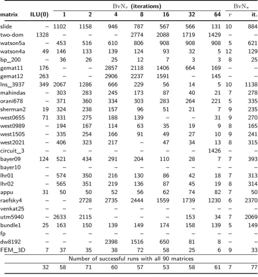
We report our experiments with GMRES and FGMRES using different permutation matrices on nonnegative matrices in Table 2. The first part of the table gives the number of GMRES iterations with the ILU(0) precondi-tioner, and with the proposed Birkhoff–von Neumann based precondiprecondi-tioner, using 𝑟 = 1, 2, 4, 8, 16, 32, and 64 permutation matrices and their coefficients. When there were less than 𝑟 permutation matrices in the BvN decomposition, we used all available permutation matrices. Note that this does not mean that we have an exact inverse, as the BvN decomposition is only approximative. We also report results with FGMRES for the BvN* preconditioners. For this case,
we give the number 𝑟 of permutation matrices used and the number of FGMRES iterations (under the column “it”). In the second part (the last row of the ta-ble), we give the number of successful runs with different preconditioners; here we also give the average number of permutation matrices in BvN* under the
column “𝑟”.
Some observations are in order. As seen in Table 2, ILU(0) results in 11 successful runs on the matrices listed in the first part of the table, and 32 successful runs in all 90 matrices. BvN𝑟preconditioners with differing number of
permutation matrices result in at least 53 successful runs in total, where BvN*
obtained the highest number of successful runs, but it has in only a few cases the least number of iterations. In 20 cases in the first part of the table, we see that adding more permutation matrices usually helps in reducing the number of iterations. This is not always the case though. We think that this is due to the preconditioner becoming badly conditioned with the increasing number of permutation matrices; if we use the full BvN decomposition, we will have the same conditioning as in 𝐴.
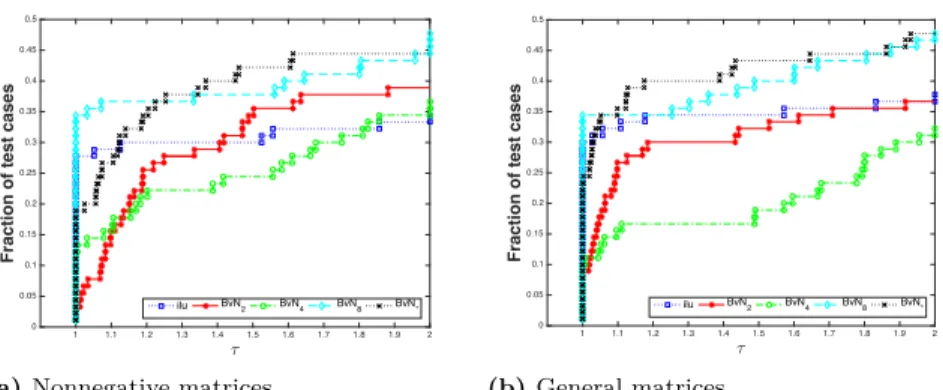
In order to clarify more, we present the performance profiles [11] for ILU(0), BvN𝑟with 𝑟 = 2, 4, 8, and BvN*in Fig. 2a. A performance profile for a
precon-ditioner shows the fraction of the test cases in which the number of (F)GMRES iterations with the preconditioner is within 𝜏 times the smallest number of (F)GMRES iterations observed (with the mentioned set of preconditioners). Therefore, the higher the profile of a preconditioner, the better is its perfor-mance. As seen in this figure, BvN* and BvN8 manifest themselves as the best
preconditioners; they are better than others after around 𝜏 = 1.1, while BvN8
being always better than others. BvN*is a little behind ILU(0) at the beginning
but then catches up with BvN8at around 1.2 and finishes as the best alternative.
Although we are mostly concerned with robustness of the proposed precon-ditioners and their potential for parallel computing, we give a few running time
Table 2. The number of GMRES iterations with ILU(0) and BvN𝑟with different number of permutation matrices, and the number of permutation matrices and FGMRES iterations with BvN*. (F)GMRES are run with tolerance 10−6, without restart and with at most 3000 iterations. The symbol “–” flags the cases where (F)GMRES were unsuccessful. All
matri-ces are nonnegative.
BvN𝑟 (iterations) BvN*
matrix ILU(0) 1 2 4 8 16 32 64 𝑟 it.
slide – 1102 1158 946 787 567 566 131 10 884 two-dom 1328 – – – 2774 2088 1719 1429 – – watson5a – 453 516 610 806 908 908 908 5 621 watson4a 49 146 133 139 124 93 32 5 12 129 bp_200 – 36 26 25 12 7 3 3 8 25 gemat11 176 – – 2857 2118 1406 664 169 – – gemat12 263 – – 2906 2237 1591 – 145 – – lns_3937 349 2067 1286 666 229 56 14 5 10 1138 mahindas – 303 283 245 173 87 40 21 7 278 orani678 – 371 360 334 303 283 264 221 5 335 sherman2 19 324 238 157 96 51 21 7 9 235 west0655 71 331 275 188 139 – – 31 9 270 west0989 – 194 167 114 63 35 19 9 8 165 west1505 – 335 254 166 91 49 27 10 9 241 west2021 – 406 323 217 – 47 34 13 8 315 circuit_3 – – – – – – – 1426 – – bayer09 124 521 434 291 204 110 28 7 7 393 bayer10 – – – – – – – – – – lhr01 – 574 350 216 130 86 42 18 7 313 lhr02 – 565 351 219 136 87 45 19 8 314 appu 31 50 50 52 56 62 74 82 7 50 raefsky4 – – 2728 2735 2444 1559 1739 1230 6 2370 venkat25 – – – – – – – – – – utm5940 – 2633 2115 – – – 153 34 7 2069 bundle1 25 163 150 139 149 174 158 139 5 149 fp – – – – – – – – – – dw8192 – – – 2398 1516 650 81 8 – – FEM_3D 7 37 35 38 72 58 25 6 9 33
Number of successful runs with all 90 matrices
1 1.1 1.2 1.3 1.4 1.5 1.6 1.7 1.8 1.9 2 = 0 0.05 0.1 0.15 0.2 0.25 0.3 0.35 0.4 0.45 0.5
Fraction of test cases
ilu BvN2 BvN4 BvN8 BvN*
(a) Nonnegative matrices
1 1.1 1.2 1.3 1.4 1.5 1.6 1.7 1.8 1.9 2 = 0 0.05 0.1 0.15 0.2 0.25 0.3 0.35 0.4 0.45 0.5
Fraction of test cases
ilu BvN
2 BvN4 BvN8 BvN*
(b) General matrices
Fig. 2. Performance profiles for the number of iterations with ILU(0), BvN𝑟 with 𝑟 = 2, 4, 8, and BvN*.
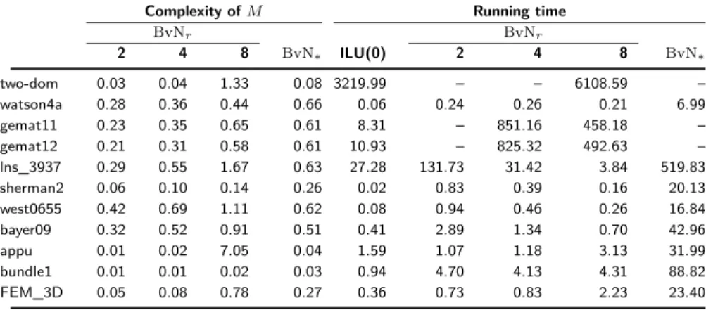
results on a sequential Matlab environment (on a core of an Intel Xeon E5-2695 with 2.30 GHz clock speed). We present the complexity of the preconditioners and the running time of (F)GMRES (total time spent in the iterations) for the cases where ILU(0) resulted in convergence in Table 3. This set of matrices is chosen to give the running time of (F)GMRES with all preconditioners under study. Otherwise, it is not very meaningful to use sophisticated preconditioners when ILU(0) is effective. Furthermore, the applications of ILU(0) and BvN𝑟
re-quire triangular solves, which are efficiently implemented in MATLAB. On the other hand, the application of BvN* requires permutations and scaling, which
should be very efficient in parallel. The running time given in the right side of Table 3 should not be taken at face value. The complexities of BvN𝑟are given as
the ratio (nnz(𝐿+𝑈 )−𝑛)/ nnz(𝐴), where 𝐿 and 𝑈 are the factors of the precondi-tioner. In this setting, ILU(0) has always a complexity of 1.0. The complexity of BvN*is given as nnz(𝑀 )/ nnz(𝐴). As seen in this table, the LU-factors of BvN𝑟
with 𝑟 ≤ 8 have reasonable number of nonzeros; the complexity of the precon-ditioners is less than one in all cases except two-dom, lns_3937, west0655, and appu. In some preliminary experiments, we have seen large numbers when
𝑟 ≥ 16. This was especially important for appu where the full LU factorization
of 𝐴 contained 85.67 · nnz(𝐴) nonzeros and 𝑀 suffered large fill-in. We run the solver with a large error tolerance of 1.0e-1, as this was enough to get the outer FGMRES to converge. The outer FGMRES iterations would change if a lower error tolerance is used in the inner solver, but we do not dwell into this issue here. With the specified parameters, an application of BvN* required, for the
Table 3. The complexity of the preconditioners and the running time of the solver. The
complexities of BvN𝑟 are given as the ratio (nnz(𝐿 + 𝑈 ) − 𝑛)/ nnz, where 𝐿 and 𝑈 are the factors of the preconditioner (ILU(0) has a complexity of 1.0), and that of BvN*is given as nnz(𝑀 )/ nnz(𝐴). A sign of “–” in the running time column flags the cases where (F)GMRES were unsuccessful. All matrices are nonnegative.
Complexity of 𝑀 Running time
BvN𝑟 BvN𝑟 2 4 8 BvN* ILU(0) 2 4 8 BvN* two-dom 0.03 0.04 1.33 0.08 3219.99 – – 6108.59 – watson4a 0.28 0.36 0.44 0.66 0.06 0.24 0.26 0.21 6.99 gemat11 0.23 0.35 0.65 0.61 8.31 – 851.16 458.18 – gemat12 0.21 0.31 0.58 0.61 10.93 – 825.32 492.63 – lns_3937 0.29 0.55 1.67 0.63 27.28 131.73 31.42 3.84 519.83 sherman2 0.06 0.10 0.14 0.26 0.02 0.83 0.39 0.16 20.13 west0655 0.42 0.69 1.11 0.62 0.08 0.94 0.46 0.26 16.84 bayer09 0.32 0.52 0.91 0.51 0.41 2.89 1.34 0.70 42.96 appu 0.01 0.02 7.05 0.04 1.59 1.07 1.18 3.13 31.99 bundle1 0.01 0.01 0.02 0.03 0.94 4.70 4.13 4.31 88.82 FEM_3D 0.05 0.08 0.78 0.27 0.36 0.73 0.83 2.23 23.40
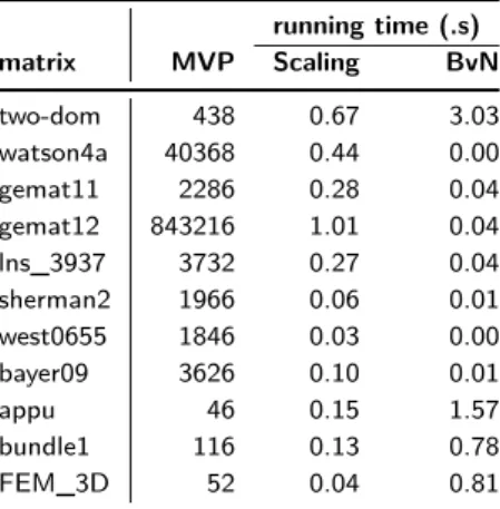
We now comment on the running time of the preconditioner set up phase. The first step is to apply the scaling method of Knight and Ruiz [20]. The dominant cost in this step is sparse matrix-vector and sparse matrix transpose-vector multiply operations. The second step is to obtain a BvN decomposi-tion, or a partial one, using the algorithms for the bottleneck matching problem from MC64 [13, 14]; these algorithms are highly efficient. The number of sparse matrix-vector and sparse matrix transpose-vector multiply operations (MVP) in the scaling algorithm, the running time of the scaling algorithm with the pre-vious setting, and the running time of the partial BvN decomposition with 16 permutation matrices are shown for the same set of matrices in Table 4. Since an application of BvN*required between 128 and 162 iterations, and those
iter-ations are no more costly than sparse matrix vector operiter-ations, we could relate the running time of FGMRES with BvN*in Table 3 to the scaling algorithm. For
example, for lns_3937 a matrix vector multiplication should not cost more than 0.27/3732 seconds, while the application of BvN* required a total of 1138 · 152
steps of inner solver. In principle the total cost of the inner solver should be around 12.5, but in Table 3, we see 519.83 seconds of total FGMRES time. As seen in Table 4, for this set of matrices the scaling algorithm and the partial BvN decomposition algorithms are fast. There are efficient parallel scaling
algo-Table 4. The total number of sparse matrix-vector and sparse matrix transpose-vector
mul-tiply operations (MVP) in the scaling algorithm, the running time of the scaling algorithm and the partial BvN decomposition algorithm in seconds.
running time (.s) matrix MVP Scaling BvN two-dom 438 0.67 3.03 watson4a 40368 0.44 0.00 gemat11 2286 0.28 0.04 gemat12 843216 1.01 0.04 lns_3937 3732 0.27 0.04 sherman2 1966 0.06 0.01 west0655 1846 0.03 0.00 bayer09 3626 0.10 0.01 appu 46 0.15 1.57 bundle1 116 0.13 0.78 FEM_3D 52 0.04 0.81
rithms [1], and the one that we used [20] can also be efficiently parallelized by tapping into the parallel sparse matrix vector multiplication algorithms.
4.2 General matrices
In this set of experiments, we used the matrices listed before, while retaining the sign of the nonzero entries. We used the same scaling algorithm as in the previous section and the proposed generalized BvN decomposition (Section 3.5) to construct the preconditioners. As in the previous subsection, we report our experiments with GMRES and FGMRES using different permutation matrices in Table 5. In particular, we report the number of GMRES iterations with the ILU(0) preconditioner, and with the proposed Birkhoff–von Neumann based pre-conditioner, using 𝑟 = 1, 2, 4, 8, 16, 32, and 64 permutation matrices and their coefficients. We also report results with FGMRES for the BvN*preconditioners.
Again, the number 𝑟 of permutation matrices used and the number of FGMRES iterations (under the column “it.”) are given for BvN*. The last row of the table
gives the number of successful runs with different preconditioners in all 90 ma-trices; here the average number of permutation matrices in BvN* is also given
under the column “𝑟". We again use the performance profiles shown in Fig. 2b to see the effects of the preconditioners. As seen in this table and the associ-ated performance profile, the preconditioners behave much like they do in the
nonnegative case. In particular, BvN* and BvN8 deliver the best performance
in terms of number of iterations, followed by ILU(0).
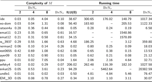
We also give the complexity of the preconditioners and the running time of (F)GMRES (total time spent in the iterations) for the cases where ILU(0) resulted in convergence in Table 6. The complexities of the preconditioners re-main virtually the same, as expected. As before, the running time is just to give a rough idea in a sequential MATLAB environment. We note that BvN*
required, on average, between 125 and 151 inner iterations. Finally note that nothing changes for the scaling and BvN decomposition algorithms with respect to the nonnegative case (Table 4 remains as it is for the general case).
4.3 Further investigations
Here, we give some further experiments to shed light into the behavior of the pro-posed preconditioners. We compare BvN*with BvN𝑟having the same number of
permutation matrices. For this purpose, we created a BvN* preconditioner and
used the number 𝑟 of its permutation matrices to create another preconditioner BvN𝑟by just taking the first 𝑟 permutation matrices from a BvN decomposition
obtained by Algorithm 1. The results are shown in Table 7, where we give the sum of the coefficients used in constructing the preconditioners and the number of (F)GMRES iterations for a subset of matrices from Table 6, where BvN* led
to a short running time.
As seen in Table 7, BvN𝑟has a larger sum of coefficients than BvN* with
the same number 𝑟 of permutation matrices. This is expected as the Algorithm 1 finds coefficients in a non-increasing order; hence the first 𝑟 coefficients are the largest 𝑟 ones. The number of (F)GMRES iterations is usually inversely propor-tional to the sum of the coefficients; a higher sum of coefficients usually results in a smaller number of iterations for the same matrix.
5 Conclusions and open questions
We introduced a class of preconditioners for general sparse matrices based on the Birkhoff–von Neumann decomposition of doubly stochastic matrices. These preconditioners are aimed primarily at solving challenging linear systems with highly unstructured and indefinite coefficient matrices in parallel computing en-vironments. We presented some theoretical results and numerical experiments on linear systems from a variety of applications. We regard this work to be a proof
Table 5. The number of GMRES iterations with different number of permutation matrices
in 𝑀 with tolerance 10−6. We ran GMRES (without restart) for at most 3000 iterations; the symbol “–” flags cases where GMRES did not converge to the required tolerance.
Ma-trices have negative and positive entries.
BvN𝑟 it. BvN*
matrix ILU(0) 1 2 4 8 16 32 64 𝑟 it.
slide 208 1051 999 745 685 490 783 659 10 663 two-dom 149 579 553 – 610 607 432 360 7 573 watson5a – 805 839 883 1094 1068 1068 1068 5 947 watson4a 48 160 149 135 120 81 34 5 12 124 bp_200 – 35 26 22 11 6 3 3 8 24 gemat11 239 – – – 2486 1588 750 152 – – gemat12 344 – – – 2607 1615 – – – – lns_3937 134 1710 969 – 121 23 9 4 10 879 mahindas – 259 232 180 121 51 – 12 7 232 orani678 – 356 341 320 288 – 225 196 5 316 sherman2 18 327 234 116 65 31 16 8 9 225 west0655 50 298 229 164 101 64 30 – 9 222 west0989 – 199 165 113 63 37 19 8 8 166 west1505 – 343 262 170 92 49 27 12 9 256 west2021 – 411 323 225 115 48 28 12 8 316 circuit_3 – – – – – – – 1178 – – bayer09 39 312 193 105 58 – 11 5 7 213 bayer10 – – 2624 2517 2517 2517 2517 2517 3 2594 lhr01 – 495 314 – 117 65 28 14 7 279 lhr02 – 508 315 – 119 67 28 15 8 277 appu 31 50 50 52 56 62 74 82 7 51 raefsky4 499 1207 722 472 592 403 860 617 6 656 venkat25 163 – – 1863 – – 258 – 8 2493 utm5940 – 1972 1588 1173 787 536 196 34 7 1520 bundle1 18 130 123 115 127 137 129 102 5 125 fp – – 2953 – – – 120 185 6 2779 dw8192 – – – 2450 1536 661 82 11 – – FEM_3D 7 42 40 40 74 62 27 6 9 38
Number of successful runs with all 90 matrices
Table 6. The complexity of the preconditioners and the running time of the solver. The
complexities of BvN𝑟 are given as the ratio (nnz(𝐿 + 𝑈 ) − 𝑛)/ nnz, where 𝐿 and 𝑈 are the factors of the preconditioner (ILU(0) has a complexity of 1.0), and that of BvN*is given as nnz(𝑀 )/ nnz(𝐴). The symbol “–” in the running time column flags the cases where (F)GMRES were unsuccessful. Matrices have negative and positive entries.
Complexity of 𝑀 Running time
BvN𝑟 BvN𝑟 2 4 8 BvN* ILU(0) 2 4 8 BvN* slide 0.03 0.05 4.04 0.10 38.67 300.65 176.02 148.79 1017.34 two-dom 0.03 0.04 1.31 0.08 56.40 183.60 – 205.53 1122.33 watson4a 0.28 0.36 0.44 0.66 0.05 0.28 0.24 0.19 6.58 gemat11 0.23 0.35 0.65 0.61 16.57 – – 1548.86 – gemat12 0.21 0.31 0.58 0.61 34.15 – – 1578.89 – lns_3937 0.29 0.55 1.66 0.63 4.68 186.25 – 3.12 359.80 sherman2 0.06 0.10 0.14 0.26 0.02 0.80 0.25 0.09 18.03 west0655 0.42 0.69 1.08 0.62 0.06 0.65 0.38 0.15 13.53 bayer09 0.32 0.52 0.90 0.51 0.05 0.62 0.21 0.08 21.12 appu 0.01 0.02 7.05 0.04 1.64 2.06 2.16 4.64 32.71 raefsky4 0.02 0.02 0.29 0.07 206.02 262.48 116.39 182.10 1027.58 venkat25 0.05 0.53 3.61 0.23 94.29 – 5462.64 – 20382.59 bundle1 0.01 0.01 0.02 0.03 0.50 4.81 4.84 5.46 76.47 FEM_3D 0.05 0.08 0.78 0.27 0.34 1.10 1.10 3.11 30.07
Table 7. Comparing BvN*with BvN𝑟having the same number of permutation matrices in terms of the sum of the coefficient of permutation matrices and the number of (F)GMRES iterations (it.). Matrices have negative and positive entries.
∑︀ 𝛼𝑖 it. matrix BvN* BvN𝑟 BvN* BvN𝑟 watson4a 0.43 0.57 124 111 lns_3937 0.29 0.80 881 68 sherman2 0.24 0.61 226 59 west0655 0.12 0.45 222 97 bayer09 0.19 0.50 216 59 appu 0.09 0.13 50 55 bundle1 0.01 0.01 125 110 FEM_3D 0.35 0.55 39 79
of concept realization; many challenging questions remain to be investigated to render the proposed preconditioners competitive with the standard approaches. Based on our current theoretical findings, we suggest the use of proposed preconditioners within a Krylov subspace method. There are two ways to go about this. In the first one, the preconditioners are built to satisfy a sufficiency condition that we identified (Theorem 4). This way, the application of the pre-conditioner requires a small number of highly concurrent steps, where there is no data dependency within a step. In the second alternative, one obtains the LU decomposition of the preconditioners that are built arbitrarily. Here, the proposed preconditioner is therefore constructed as a complete factorization of an incomplete matrix. We demonstrated that using around eight matrices is good enough for this purpose. Beyond that number, the LU decomposition of the preconditioner can become a bottleneck (but remains always cheaper than that of the original matrix). Is there a special way to order these preconditioners for smaller fill-in?
The construction of the preconditioners needs an efficient doubly stochastic scaling algorithm. The known algorithms for this purpose are iterative schemes whose computational cores are sparse matrix-vector multiply operations whose efficient parallelization is well known. For constructing these preconditioners, we then need a bottleneck matching algorithm. The exact algorithms for this pur-pose are efficient on sequential execution environments, but hard to parallelize efficiently. There are efficiently parallel heuristics for matching problems [18], and more research is needed to parallelize the heuristic for obtaining a BvN decomposition while keeping an eye on the quality of the preconditioner.
Acknowledgment: The work of Michele Benzi was supported in part by NSF
grant DMS-1418889. Bora Uçar was supported in part by French National Re-search Agency (ANR) project SOLHAR (ANR-13-MONU-0007). We thank Alex Pothen for his contributions to this work. This work resulted from the collabo-rative environment offered by the Dagstuhl Seminar 14461 on High-performance Graph Algorithms and Applications in Computational Science (November 9–14, 2014).
References
[1] P. R. Amestoy, I. S. Duff, D. Ruiz, and B. Uçar. A parallel matrix scaling algorithm. In J. M. Palma, P. R. Amestoy, M. Daydé, M. Mattoso, and J. C. Lopes, editors, High
Interna-tional Conference, volume 5336 of Lecture Notes in Computer Science, pages 301–313.
Springer Berlin / Heidelberg, 2008.
[2] H. Anzt, E. Chow, and J. Dongarra. Iterative sparse triangular solves for precondition-ing. In Jesper Larsson Träff, Sascha Hunold, and Francesco Versaci, editors, Euro-Par
2015, pages 650–661. Springer Berlin Heidelberg, 2015.
[3] M. Benzi, J. C. Haws, and M. T uma. Preconditioning highly indefinite and nonsym-metric matrices. SIAM journal on Scientific Computing, 22(4):1333–1353, 2000. [4] G. Birkhoff. Tres observaciones sobre el algebra lineal. Univ. Nac. Tucumán Rev. Ser.
A, (5):147–150, 1946.
[5] R. A. Brualdi. Notes on the Birkhoff algorithm for doubly stochastic matrices.
Cana-dian Mathematical Bulletin, 25(2):191–199, 1982.
[6] R. A. Brualdi and P. M. Gibson. Convex polyhedra of doubly stochastic matrices: I. Applications of the permanent function. journal of Combinatorial Theory, Series A, 22(2):194–230, 1977.
[7] R. A. Brualdi and H. J. Ryser. Combinatorial Matrix Theory, volume 39 of
Encyclope-dia of Mathematics and its Applications. Cambridge University Press, Cambridge, UK;
New York, USA; Melbourne, Australia, 1991.
[8] R. Burkard, M. Dell’Amico, and S. Martello. Assignment Problems. SIAM, Philadel-phia, PA, USA, 2009.
[9] E. Chow and A. Patel. Fine-grained parallel incomplete LU factorization. SIAM journal
on Scientific Computing, 37(2):C169–C193, 2015.
[10] T. A. Davis and Y. Hu. The University of Florida sparse matrix collection. ACM
Transactions on Mathematical Software, 38(1):1:1–1:25, 2011.
[11] E. D. Dolan and J. J. Moré. Benchmarking optimization software with performance profiles. Mathematical Programming, 91(2):201–213, 2002.
[12] I. S. Duff, A. M. Erisman, and J. K. Reid. Direct Methods for Sparse Matrices. Oxford University Press, London, 1986. In preprint of second edition. To appear.
[13] I. S. Duff and J. Koster. The design and use of algorithms for permuting large entries to the diagonal of sparse matrices. SIAM journal on Matrix Analysis and Applications, 20(4):889–901, 1999.
[14] I. S. Duff and J. Koster. On algorithms for permuting large entries to the diagonal of a sparse matrix. SIAM journal on Matrix Analysis and Applications, 22:973–996, 2001. [15] F. Dufossé and B. Uçar. Notes on Birkhoff–von Neumann decomposition of doubly
stochastic matrices. Linear Algebra and its Applications, 497:108–115, 2016. [16] H. N. Gabow and R. E. Tarjan. Algorithms for two bottleneck optimization problems.
J. Algorithms, 9(3):411–417, 1988.
[17] F. R. Gantmacher. The Theory of Matrices, volume 2. Chelsea Publishing Co.„ New York, NY, 1959.
[18] M. Halappanavar, A. Pothen, A. Azad, F. Manne, J. Langguth, and A. M. Khan. Codesign lessons learned from implementing graph matching on multithreaded ar-chitectures. IEEE Computer, 48(8):46–55, 2015.
[19] R. A. Horn and C. R. Johnson. Matrix Analysis. Cambridge University Press, second edition, 2013.
[20] P. A. Knight and D. Ruiz. A fast algorithm for matrix balancing. IMA journal of
Numerical Analysis, 33(3):1029–1047, 2013.
[21] P. A. Knight, D. Ruiz, and B. Uçar. A symmetry preserving algorithm for matrix scal-ing. SIAM journal on Matrix Analysis and Applications, 35(3):931–955, 2014.
[22] M. Manguoglu, M. Koyutürk, A. H. Sameh, and A. Grama. Weighted matrix ordering and parallel banded preconditioners for iterative linear system solvers. SIAM journal on
Scientific Computing, 32(3):1201–1216, 2010.
[23] Y. Saad. A flexible inner-outer preconditioned GMRES algorithm. SIAM journal on
Scientific Computing, 14(2):461–469, 1993.
[24] R. Sinkhorn and P. Knopp. Concerning nonnegative matrices and doubly stochastic matrices. Pacific J. Math., 21:343–348, 1967.
[25] R. S. Varga. Matrix Iterative Analysis. Springer, Berlin, Heidelberg, New York, sec-ond (revised and expanded edition of prentice-hall, englewood cliffs, new jersey, 1962) edition, 2000.