HAL Id: hal-01342876
https://hal.archives-ouvertes.fr/hal-01342876
Submitted on 6 Jul 2016HAL is a multi-disciplinary open access archive for the deposit and dissemination of sci-entific research documents, whether they are pub-lished or not. The documents may come from teaching and research institutions in France or abroad, or from public or private research centers.
L’archive ouverte pluridisciplinaire HAL, est destinée au dépôt et à la diffusion de documents scientifiques de niveau recherche, publiés ou non, émanant des établissements d’enseignement et de recherche français ou étrangers, des laboratoires publics ou privés.
SVM CLASSIFICATION OF QUASI-PERIODIC
REGIMES OF SINGLE REED INSTRUMENTS
Jean-Baptiste Doc, Christophe Vergez, Samy Missoum
To cite this version:
Jean-Baptiste Doc, Christophe Vergez, Samy Missoum. SVM CLASSIFICATION OF QUASI-PERIODIC REGIMES OF SINGLE REED INSTRUMENTS. ACOUSTIS’2013 NEW-DELHI, 2013, New-Delhi, India. �hal-01342876�
SVM CLASSIFICATION OF QUASI-PERIODIC REGIMES
OF SINGLE REED INSTRUMENTS
Jean-Baptiste DOC, Christophe VERGEZ,
Laboratoire de Mécanique et d'Acoustique, LMA CNRS UPR7051, Marseille, 13402 Cedex 20 France
e-mail: jbdoc@lma.cnrs-mrs.fr
and Samy MISSOUM
Computational Optimal Design of Engineering Systems (CODES) Laboratory Department of Aerospace and Mechanical Engineering
University of Arizona Tucson, Arizona 85721
Abstract
Single-reed instruments can produce multiphonic sounds when they generate quasi-periodic oscilla-tion regimes. An approach to map the periodic and quasi-periodic regimes of a wind instrument is presented. The mapping is performed using an SVM classifier trained using the output of a simpli-fied single-reed instrument model. The SVM classifier is iteratively refined using an adaptive sampling scheme referred to as Explicit Design Space Decomposition. This method provides the ex-plicit boundaries separating quasi-periodic and periodic regimes and highlights the influence of key parameters involved in the production of multiphonic sounds.
1 - Introduction
For wind instruments, the inharmonicity of resonance frequencies is an important criterion in instru-ment-making. This may affect, for example, the tone color or the tuning of the instrument [1]. For an instrument like the saxophone, the inharmonicity of the resonance frequencies is largely inherent in the constitution of the instrument (side holes, truncation of the cone).
The single reed instruments can be considered as self-oscillators. Through a valve effect, the mouthpiece ensures the conversion of a static pressure (in the mouth) into an alternating pressure (inside the mouthpiece) which is sustained by the acoustic feedback of the air column inside the bore. The air flow within the instrument is non-linearly related to the static pressure set by the musi-cian. Therefore, the single-reed instruments are commonly modelled as nonlinear dynamical sys-tems. The natural frequencies of the bore being inharmonic, the self-oscillator can produce complex oscillation regimes. Among these, quasi-periodic oscillations have the particularity of being
com-posed at least of two incommensurable frequencies [2]. This type of oscillation corresponds to mul-tiphonic sounds.
The quasi-periodic regimes produced by wind instruments are rarely studied in the literature and not completely understood. Therefore, the two aims of this work are : - to identify the simplest model of single reed instruments (in terms of number of degrees of freedom) capable of reproducing quasi-periodic regimes; - to analyze, for this model, the parameters values giving rise to quasi-quasi-periodic re-gimes.
The following model is tested : only the first two eigen modes of the resonator are taken into account and the reed dynamic is ignored, whereas the air flow depends on the square root of the pressure difference across the reed, and on the opening of the reed channel.
To identify the conditions for which quasi-periodic regimes emerge, we investigate the influ-ence of control parameters (blowing pressure, mouthpiece parameter) and design parameters (para-meters of the two modes, including inharmonicity). For this, a method called Explicit Design Space Decomposition is used to classify the oscillation regimes according to the different parameters val-ues. A Support Vector Machine classifier allows finding explicitly the boundary between periodic and quasi-periodic regimes with respect to the parameters considered.
The paper is structured as follows. At first, the single-reed instrument model is presented. In a second time, the classification method of oscillating regimes is detailed. In the last part, results are presented.
2 - Classical single-reed instrument model
2.1 – Continuous time equation
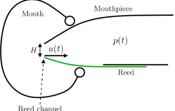
By blowing air into the instrument through the reed channel, the player destabilizes the reed from its rest position (see Figure 1). The acoustic response of the instrument acts as a feedback loop which influences the reed position. The production of a sound corresponds to the self-sustained os-cillation of this dynamical system. The reed can be modeled as a mass/spring/damper oscillator. However, because its resonance frequency is large compared to the first harmonics of typical play-ing frequencies, inertia and dampplay-ing of the reed are ignored in this paper.
Considering as a reference the minimum pressure pM=KH required to close the reed channel in the non-oscillating case (where K is the reed stiffness per unit area and H is the height of the reed channel at rest), we introduce the following dimensionless quantities for pressure in the mouth and in the mouthpiece and for the volume flow through the reed channel respectively [3] (see Figure 1) :
γ= pm pM , p(t )= ̃ p(t ) pM , u(t )= Zc̃u (t ) pM (1) where Zc=ρc
S is the characteristic impedance for plane wave inside the resonator of cross section S , ρ is the air density and c is the sound speed. Likewise it is convenient to define a dimension-less reed opening parameter :
ζ=ZcWH
√
2ρpM (2)
where W is the width of the reed. The two dimensionless parameters controlled by the musician for a given fingering are γ and ζ , the blowing pressure and an mouthpiece parameter respectively.
Mainly based on considerations from Hirschberg [4], an explicit expression for the air flow u is given below :
u=ζ(1−γ+ p)
√
∣γ− p∣sign(γ− p) if γ− p ⩽1u=0 if γ− p>1 (3)
The first equation corresponds to the case of an open reed channel. In that case, the incoming air flow depends only on the pressure drop γ− p between the mouth and the mouthpiece. When the tip of the reed gets in contact with the lay, it completely closes the reed channel, therefore canceling the air flow, which is expressed by the second equation.
The input impedance of the instrument, denoted Z(ω) , is defined in the frequency domain as the ratio between the pressure P(ω) and the air flow U(ω) into the mouthpiece. It can be written as the modal expansion :
Z(ω)=jω
∑
n Fn ωn2−ω2+jωω n/Qn (4) where ωn is the natural pulsation, Qn is the quality factor and Fn is the modal factor of the nthresonance. Simplification is obtained by truncating the series. To obtain a simple model (in terms of degrees of freedom), the series (4) is truncated at the second order ( n= 2 ) which is the minimum condition to expect quasi-periodic oscillations. The inverse Fourier transform of the truncated series allows modelling a reed instrument as a self-sustained oscillator defined by the following coupled system : d2 dt2 p1(t )+ ω1 Q1 d dt p1(t )+ω1 2 p1(t )=F1 d dtu(t ) d2 dt2 p2(t)+ ω2 Q2 d dt p2(t )+ω2 2p 2(t)=F2 d dtu(t) (5) The pressure inside the mouthpiece p(t) is defined as the sum of the two components p1(t) and
p2(t ) . The modal parameters used thereafter are F1=687 , F2=1088 , Q1=21.5 , Q2=33.9 ,
ω1=539.4 and ω2=1348.4 . The quality factors and the first modal factor and the first frequency
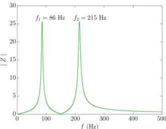
resonance correspond to a cylindrical tube of radius r=7.5mm and a length l=1m . The parameter F2 is fixed in order to impose the same amplitude for the two first impedance peaks (see Figure 2). The frequency ω2 is chosen to obtain an inharmonicity
ω2
ω1=2.5 (see Figure 2).
2.2 - Numerical aspects
The system of equations (5) is solved using an ordinary differential equation solver. As multiple time scales are involved in the problem (duration of blowing pressure transient, bore resonance frequencies ...) and since the equations are not the same when the reed channel is closed or open, an ODE solver designed for stiff problems, namely ode23s from the Matlab ODE Suite is used.
Figure 1: Schematic representation of a musician playing a single-reed instrument
Using a solver requires the setting of initial states of the dynamical system (5). The pressure inside the mouthpiece at the onset of sound production is still not well understood. Therefore, the initial conditions used for the resolution of the model are chosen arbitrarily. A pressure is imposed at time t=0 on the first mode of the bore, which is represented by the condition p1=0.01 . The
other initial conditions are imposed to be zero.
3 - Classification of oscillation regimes
3.1 - Criterion to identify quasi-periodic regimes
The mouthpiece pressure is the signal chosen to test quasi-periodicity of the regime. More precisely, the discriminating quantity is its power envelope, denoted pwr (obtained with the toolbox YIN [5] in this paper). For a periodic signal, the power envelope does not vary significantly in the steady part of the sound. Contrary to a quasi-periodic signal whose power envelope varies especially as these beats have large amplitude. On the basis of this observation, the following descriptor ε is introduced :
ε=Var( pwr)
〈
pwr〉
(6)where Var ( pwr) and
〈
pwr〉
are the variance and the mean of signal pwr respectively. The descriptor ε is calculated from a stationary part of the pressure signal, that is the second half of the pressure signal. After a parametric study, it is found that beyond the threshold 1.10−2% , the descriptor ε systematically describes a quasi-periodic pressure signal.Therefore, the following cri-terion is retained : - ε<1.10−2% the signal is tagged "periodic"; - ε⩾1.10−2% the signal is tagged "quasi-periodic".3.2 - SVM classification
A technique referred to as Explicit Design Space Decomposition, called EDSD [6], is presented be-low. The basic idea is to construct the boundaries of an n-dimensional map using a Support Vector Machine (SVM) [7], which provides an explicit expression of the boundary in terms of the chosen parameters. SVM is a machine learning technique that is widely used for classification. In optimiza-tion and reliability assessment, SVM is used to approximate highly nonlinear constraints and limit-state functions. The most important features of SVMs are their ability to handle multiple criteria us-ing a sus-ingle classifier, to be insensitive to discontinuities, and to be computationally very efficient. The ability of a SVM to handle discontinuities is essential in the case of sudden changes in the nature of oscillation regimes.
Figure 2: Modulus of the input impedance of the resonator modeled with the modal parameters : F1=687,F2=1088,Q1=21.5,Q2=33.9,ω1=539.4 and ω2=1348.4
An initial approximation of the map is obtained using a design of experiments (DOE) such as Latin Hypercube Sampling (LHS) of the parameters. These DOE techniques are tailored so as to provide information over the whole space using a reasonable number of samples in higher dimen-sions. The initial approximation of the boundary using a DOE might not be accurate and needs to be refined while maintaining a reasonable number of resolution of the single-reed instrument model. This refinement is performed using an adaptive sampling scheme that is described in [6].
4 - Results
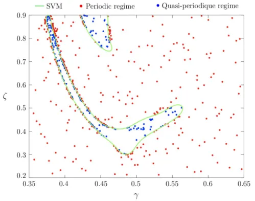
Figure 3 highlights three different area into the parameter space (γ , ζ) . Represented by a green line, the SVM is the boundary separating periodic and quasi-periodic oscillation regimes. One can see two different areas of quasi-periodic oscillations. This map was obtained with 200 initial points, distributed throughout the parameter space. Additionally, 300 adaptive points were used to de-scribed the complex shape of the two boundaries.
The 500 total samples used to make this map allows a precise definition of the complex shape of the boundaries. The adaptive samples are concentrated around the border described by the SVM, which comes from the adaptive sampling scheme [6]. Such a density of points could not have been imposed uniformly across the parameter space, which underlines why the adaptive aspect of the classification method is essential to evaluate precisely these regions of quasi-periodicity.
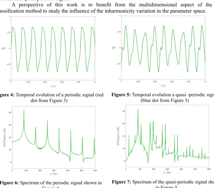
Figure 4 and Figure 5 show typical periodic and quasi-periodic signals, taken from the map in Figure 3. One can see that the periodic signal is characterized by a spectrum built around a fundamental frequency (see Figure 6). Furthermore, the quasi-periodic signal is characterized by a spectrum built around two incommensurate frequencies (see Figure 7).
5 - Conclusion
A first conclusion is that the basic model considered in this paper is able to produce quasi-periodic sounds. Since the mass and the damping of the reed are ignored, and only two modes of the reson-ator are retained, it is probability the minimal model in terms of number of degrees of freedom cap-able of producing quasi-periodic sounds.
Figure 3: Detection of quasi-periodic regimes. The boundaries between periodic and quasi-periodic regimes (green line) is obtained using SVM with adaptive sampling (200 initial points and 300 adaptive points).
Classification through the EDSD approach proved to be an effective and efficient way of highlighting a desired behaviour, namely quasi-periodic, in a multidimensional parameter space. Moreover the choice of the magnitude variation of the power envelope is relevant to distinguish periodic and quasi-periodic signal.
A perspective of this work is to benefit from the multidimensional aspect of the classification method to study the influence of the inharmonicity variation in the parameter space.
References
[1] J.P. Dalmont, B. Gazengel, J. Gilbert et J. Kergomard : Some aspects of tuning and clean
intonation in reed instruments. Applied Acoustics, 46(1):19–60, 1995.
[2] V. Gibiat : Phase space representations of acoustical musical signals. Journal of Sound and Vibration, 123(3):529 – 536, 1988.
[3] F. Silva, V. Debut, J. Kergomard, C. Vergez, A. Deblevid et P. Guillemain : Simulation of single reed instruments oscillations based on modal decomposition of bore and reed dynamics. In
Proceedings of the International Congress of Acoustics, Sept 2007.
[4] A. Hirschberg : Aero-Acoustics of Wind Instruments. In G. Weinreich, A. Hirschberg and J. Kergomard : Mechanics of Musical Instruments, volume 335 of CISM Courses and Lectures, pages 291–369. Springer-Verlag, New York, 1995.
[5] A. de Cheveigne et H. Kawahara : YIN, a fundamental frequency estimator for speech and music. J. Acoust. Soc. Am., 111(4):1917–1930, 2002.
[6] A. Basudhar et S. Missoum : An improved adaptive sampling scheme for the construction
of explicit boundaries. Structural and Multidisciplinary Optimization, pages 1–13, 2010. [7] N. Cristianini et B. Schölkopf : Support vector machines and kernel methods: The new
gen-eration of learning machines. Artificial Intelligence Magazine, 23(3):31–41, 2002.
Figure 6: Spectrum of the periodic signal shown in Figure 4
Figure 4: Temporal evolution of a periodic signal (red dot from Figure 3)
Figure 5: Temporal evolution a quasi -periodic signal (blue dot from Figure 3)
Figure 7: Spectrum of the quasi-periodic signal shown in Figure 5