A comparison of tree search schemes for decision networks

LIBRARY OF THE

MASSACHUSETTS INSTITUTE OF

TECHNOLOGY

TABLE

OF

CONTENTS

INTRODUCTION

1

THE

BRANCH

AND

BOUND

TECHNIQUE

3

FIXED

ORDER ALGORITHM

6

Feasibility Tests 7

Determination of Bounds 7

Branching and Backtracking 9

Algorithm Termination 10

Flow Chart 10

Sample Problem 11

Decision

Node

Order 14

PARTITIONING

ALGORITHM

16

Sample Problem 18

DECOMPOSITION

20

Combining Subproject Solutions 23

CONCLUSION

28

REFERENCES

29

INTRODUCTION

Decision

CPM

has been proposed

by Crowston

and

Thompson

[2]

as a

method

for the simultaneous planning and scheduling of projects.

In conventional

CPM

analysis, decisions are

made

as to the specific

method

for performing each task before the project is scheduled.

However,

decision

CPM

allows the planner to include all reasonable alternative

methods

of performing each job in the project graph, the alternatives possibly having different costs, different time durations, and different technological dependencies, and to then pick the best combination of job alternatives in light of cost and due-date considerations. In addition,

interdependency between

methods

used to complete different tasks

may

be included. Such alternative interdependencies

may

arise

from

a

requirement for consistency in the materials or designs used, for

example.

Crowston

and

Thompson

show how

Decision

CPM

networks can be

given a mathematical representation using integer variables. Crowston

also

shows

in [l] that all nondecision jobs (i.e., jobs for which there are no alternatives)

may

be eliminated

from

the original network in a fashion so that resulting "reduced network" is equivalent in the following sense:

Given a set of decisions, the resulting early start times for all decision jobs in the reduced network will be the

same

as those in the original.

The

optimal solution to the reduced network is thus optimal to the original.

The

reduced

problem

is formulated as follows: associate with

each iob S-- in the network its cost C.., its early start time w... and an integer variable d.. which takes the value 1 if the job is

performed

and

if it is not.

The

subscript "ij" indicates that a decision job is the jth

alternative for decision node i.

A

due date

DD

is

assumed

with a

premium

of "r" dollars per time period of early completion and a penalty of "p"

dollars per time period of late completion.

Then

find

D

={ d. .} so as to

m.inimize the

sum

of job cost and due-date penalty or

premium,

that is:

N

k(i) _{_ +}

Min

Z

=

2

2

d..

C.

-

rw_

₊

pw^

j=l 3=1 J J

subject to:

Interdependency

(a) Mutually exclusive:

k(i)

S

d,, = 1 1 = 1

N

j=l ^J

(b) Alternative: as required i.e.

d.. < d 13

-

mn

d.. = d 13

mn

Precedence

- _M(l - d..) +

W..+

t... , < w, ,

M="oo"

13' 13 i3kl

-

kl '"

where

S.. is an

immediate

predecessor of S, ,

13 kl

Project Completion

Wj, -

Wp

+

Wp

-

DD

=

Wp.

Wp

>

where

N

is the

number

of decision nodes; k(i) is the

number

of alternatives for decision node (i); t., , is the time required

from

the start of the predecessor S.. to the start of its

immediate

successor S, ,; and w^, is the early start time of project finish.

For

the solution procedure to be described, that is

Branch

and

Bound,

more

general objective functions

may

be easily handled.

For

example,

rewards

and penalties

may

be

associated with the completion

of particular tasks in the project [l] . It is required, however, that

Z

be

nondecreasing with completion time.

The

algorithms described in this

paper are concerned with finding the optimal solution(s) in

terms

of Z.

The

problem

of finding the project cost curve

(minimum

cost for each

possible completion date) is only slightly

more

difficult and is discussed

in [9] .

THE

BRANCH

AND

BOUND

TECHNIQUE

The method

of

Branch

and

Bound

has

been

adopted for the solution

of

DCPM

networks.

Branch

and Bound, otherwise

known

as

Combina-torial

Programming

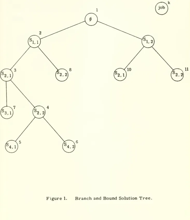
or Controlled Enumeration, is an intelligently

structured search of the space of all possible solutions.

The

procedure is based on two principal concepts: the use of a controlled enumeration

technique for (implicitly) considering all potential solutions, and the elimination

from

explicit consideration of particular potential solutions

which

are

known

from

bounding or feasibility considerations to be

unacceptable.

The

technique has been applied to a variety of problems,

most

of which require all or

mixed

integer solutions.

The method

as applied to this

problem

is illustrated

by

the tree

search

diagram

of Figure 1.

The

solution space is first partitioned into the mutually exclusive collectively exhaustive subspaces of solutions

defined

by

the choice of one of the possible alternatives for decision node I.

Then

each of these subspaces is further partitioned using another decision node. If the process is continued through all decision nodes, every

solution satisfying the mutually exclusive interdependency conditions is

obtained. In Figure 1, the case

where

there are only two alternatives for

each decision node is illustrated, but the extension to the case

where

there are k(i) alternatives for node i can be easily visualized.

A

partial solution: p is a set of n decisions d / v- » 1

—

^ _{^n a(m)j}

m

= 1, . . . , n

where

k is

some

bookkeeping label and a is

a vector of decision node labels i in

some

order.

An

It

augmentation of _p corresponds to the choice of a job alternative for decision node a (n + 1) to be done in

con-k iunction with _p J ^n k' k , Pn+1 = Pn a(n+l)j- I-k' k

A

completion: p!X of p results

from

a series of

augmenta-tions such that a decision is

made

for each node. In Figure 1,

7

the labels have been chosen so that _p„ ={d. . ; d„ .} is an

augmentation of _Pg = {d, , ; dg , } . If

N

= 4, p. and p. are

3

two possible completions of p-.

It IS important to note that a partial solution p

may

define one or

more

paths

from

start to finish in the "reduced network" of the project.

If so, a project completion date

w

is defined for the partial solution.

-job

Then

w

is a lower bound on the completion date which will result

from

k k "

any completion of _p . Similarly, the quantity

C

=

S

C.. d.. is a lower

n „ -J s,

ij jj

k

bound on the total job cost which will result

from

any completion of p .

Then

„k

„k.

k+

k-Z

=

C

+

pwp

-

rwp

is a lower bound on the objective function which will be obtained

from

any completion of p .

Suppose

some

value

Z*

is the value

Z

for the best complete

k k

solution found thus far.

Then

if

Z*

<

Z

, p is bounded and need no

n

longer be considered.

Furthermore,

all completions of p

may

be

J,

discarded. Similarly, if p can be

shown

to be infeasible

from

alternative "'

n

interdependency considerations, then it and all of its possible completions

may

be discarded.

The Branch

and

Bound

technique is a procedure for generating partial solutions by successive augmentations of the starting partial solution p (no decisions). At each stage, the current partial solution is

checked to determine whether it is bounded or infeasible. If so, it is

discarded.along with its subspace of possible completions, and another partial solution is considered.

The

process continues until the entire solution space has been explicitly or implicitly considered.

The

best feasible solution found at this point is optimal.

FIXED

ORDER

ALGORITHM

The

algorithm described in this section is

termed

"fixed order" because the order a in

which

decision nodes are processed is predetermined

and fixed.

The

essential features of the algorithm are presented in the

-following order: feasibility tests, determination of bounds, branching

and backtracking, and algorithm termination.

A

flow chart and

sample

problem

solution follow, and then

some

considerations for choice of effective order a are discussed.

Feasibility Tests

The

programmed

version of this algorithm is equipped to handle pairwise interdependency constraints of the following types:

d.. 13

representing the

minimum

total decision job cost which

must

be added to the objective function.

Z

=

_{Z min}

(C..)+

SC.

d.. + pwt, - _rw"

I ij I] 13 ^

F

F

3

This step tightens the cost portion of the lower bound for a partial solution

by

incorporating the fact that a complete solution

must

include, at least,

the cost of the cheapest job alternative for each decision node not yet considered. Since the algorithm

works

with reduced networks, the cost of nondecision jobs is assunned to

be

zero.

For

real projects, this cost

must

be added to the objective function, but it is fixed cost and has no

effect upon the workings of the algorithm.

The

"completion time" portion of the bound is determined by a standard forward pass through the network defined by the partial solution.

This is accomplished in the

programmed

version of the algorithm

by

setting d.. = for all decision jobs not selected by the partial solution,

and then conducting the forward pass calculations over only those time

constraints for which the d.. for both predecessor and successor are

positive.

The method

does not require distinguishing between those decision jobs which have not been selected because they have not yet

been considered for the current partial solution, and those rejected in

favor of another alternative job.

The

artificial start and finish jobs are

assumed

to have been selected by all solutions.

There

are

many

cases in which the completion time portion of the

bound for a partial solution p could be strengthened by taking into account decisions which

must

be

made

for decision nodes a(m),

m

> n.

For

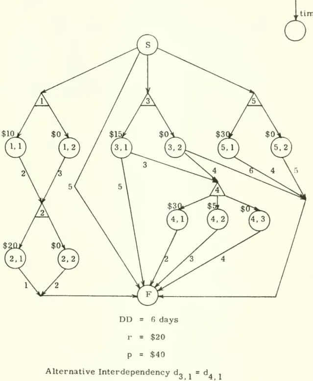
example, in Figure 2 it can be seen that a choice of S, . implies a lower

-bound on completion time of six days, even though no path exists through the network until a decision is

made

for decision node 2.

The

algorithm

does not recognize such cases; artificial nondecision jobs

may

be

inserted in the network to represent these and

more

complicated situations,

however. 4 Decision node

_/\

Precedences

Decision job ( ) Artificial job ^ , Figure 2

Branching and Backtracking

An

"iteration" for this algorithm refers to the process of picking

some

partial solution p for further elaboration, and then generating and evaluating each of the possible augmentations p

U

d.., j = 1, . . . k(i)

where

i = Qf(n + 1).

The

rule used to determine which of all active (feasible and unbounded) solutions to consider for the next interation is

the following: choose the partial solution p which has the lowest value

Z

from

the set of all active solutions

most

nearly complete. This rule

is used for both "branching" (i.e., proceeding

down

the solution tree) and "backtracking" (i.e. , proceeding back up the tree

when

the current

partial solution is completed or discarded). It can be seen that this

procedure

amounts

to picking the

most

promising of the

most

recently

generated active partial solutions and shall be referred to as a

LIFO

strategy.

The

LIFO

strategy

was

adopted primarily because it tends to

minimize computer

storage requirements.

The

strategy is

implemented

by

the maintenance of a

pushdown

list, y , of solution labels k.

Algorithm Termination

The

algorithm will terminate

when

all possible solutions have been considered explicitly or implicitly. Since there are a finite

number

of solutions, termination is guaranteed.

The

partitioning procedure is such that the entire space of potentially optinaal solutions is spanned by

the set of active partial and complete solutions.

When

the

number

of

complete solutions which have the lowest

Z

value =

Z*

is equal to the

number

of active solutions, the algorithm terminates.

Flow

Chart

The

complete fixed order algorithm operates as follows after

a

is specified:

Step I:

Z*

= 00

y = {1}

p^ = _(0). Z^ =

If

Step 2:

K

= >(1); current solution is _p .

If Z*' >

Z*,

go to Step 6.

If

Z^

<

Z

* , go to Step 3 if n < N;

Step 5 if n = N.

Step 3: I = a(n + 1)

-step 4: Evaluate each of the augmentations p

U

d.

.

3 = 1, k(i) by testing each for: a. feasible?

b. Z^' <

Z*

?

Save the solutions which pass these tests, and insert the

new

labels k' at the top of the list 7

k'

in order of nondecreaslng

Z

. If there are no

unbounded feasible solutions, go to Step 6;

otherwise go to Step 2.

Step 5:

Z*

= Z; revise 7

by

putting 7(1) at the end

and

moving

all other elements up one position.

Go

to Step 7.

Step 6: Delete 7(1)

from

7 and

move

all other elements up one position.

Step 7: Finished? If not, go to Step 2. Sample Problem

Suppose the decision node order

0=

3, 4, 1, 2. 5 is specified

the sample problem of Figure 3. Then the solution is as follows:

(1)

Z*

= 00 y = {1} Po\ - (0) (2) k = 1; current solution is _p (3) i = 3 (4) _pj = (dg j)

Wp

= 5 C^ = $15 Z^ = -$5 Pi " ^^3 2^ "^F " ^

^^

" ^°

^^

'^ ^^^ 7 = {1, 2}

Z*

= 00 11

-cost time

DD

= 6 days r = $20 p = $40 Alternative Interdependency d„ . = d. .

Figure 3.

Sample Problem.

In the next iteration, solutions {d„ i : d. „) ^"^ (^3 _{i'^4 3)} are found

to be infeasible. At the end of Step 4:

'2 = ^^3,1' ^4,1>

4

= 5

C^

= ^^5 2 Pi {d3 2}

w^

= 6

c2=$0

Z^

= $45

zr

= _$40 {1.2}

Z*

= oc

The

process continues until the only active solution is

P5 = ^^3.1= ^4.1=

^2=

^2,2= ^5,2^ "^F

^^

C

=

Z

=

$45 $25

The

solution tree is

shown

in Figure 4.

©

(5.$15,-$5) (5,$45.$25L ^4.1^ _(4,2 I 4.3] I (5, $55,

$35H(5,

$45, $25) 1,

(1^

(5, $65. $45) 1(5,$45. $25) 2,1) _(2.2) (5, $75. $55) 1(5, $45, $25) 5,1)

(Q

Optimal (w , c. Z)

016,0.0)

(7, $5, $45) I (8. $0, $80) (4,2^

(Cs)

I = infeasible

B

= bounded Figure 4, 13

Decision

Node Order

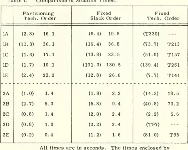
Preliminary experimentation with the fixed order algorithm

showed

that solution time for a given

problem

was

extremely sensitive to the order

of decision nodes a.

The major

portion of this variability in solution

time

seemed

to be concentrated in the time to prove optimality once the

optimal solution had been found. It

was

further observed that solution

time

was minimized

by those decision node orderings in which "critical"

nodes (i.e. , those nodes for which the chosen decision job in the optimal solution

was

on the critical path(s) )

were

processed first. With such

orderings, strong w,., bounds

were

generated near the top of the solution tree, and the tree

was

consequently

more

effectively pruned.

In order to obtain a

measure

of the potential criticality of decision nodes, the following simple heuristic

was

devised:

For

each decision

node choose the cheapest alternative. In the resulting network, calculate

the total slack for each job.

For

a job not chosen, the calculated slack is

that which would occur if the job

were

performed, but with the start times

for the chosen jobs unaltered. In

some

cases, this implies negative slack. , , 2

Choose

the decision node order

a

on the basis of increasing

mm

slack.

J

This ordering will be referred to as "slack order. "

2

This rule should perhaps be modified

somewhat.

Since the total slack calculated in this fashion is not particularly meaningful for those

decision nodes not on the original critical path, it

may

be better to order

these nodes so that they are grouped technologically. This gets

more

directly at the

problem

of ensuring that paths through the network are

defined by successive decision nodes.

The

groups of nodes can be ordered on the basis of slack for the group.

However,

this is not a

simple rule to apply for

complex

networks and has not been tested.

-The

algorithm

was programmed

in Fortran IV for an

IBM

7094

computer

and run under the time-sharing

system

of

MIT's

project

MAC.

The

program was

tested on variations of two fifteen-node,

three-15

decisions-per-node (3 possible solutions) problems.

The

two

problem

types, hereafter referred to as

Type

1 and

Type

2 problems, differed in the extent to which interconnections between opposite portions of the

network existed.

Type

2

problems

contain

many

such interconnections,

so that a

number

of competing critical paths

were

likely to develop.

Typically, nine to eleven of the decision nodes in the

problem

became

critical for

some

partial solution. Variety

was

provided to these

problems

by

altering due dates,

premiums,

penalties, and times for precedence

constraints (t ,^,). Solution times are reported in Table 1, and do not

include the three to five seconds required for input-output and initializa-tion.

Results for the fixed order algorithm are

shown

for both slack

order and technological order. Technological order offers

some

compu-k

tational efficiencies in

determining^

but is essentially a

random

order

with regard to potential criticality, and results have been included

primarily for the basis of comparison. In all cases, slack order has

proven to be superior to technological order.

It has been proposed that decision nodes involved in alternative

interdependency constraints should be placed at the top of the decision tree so as to allow effective pruning on the basis of feasibility considerations. This, however,

may

interfere with a pure slack order, and results with a few test

problems

indicate that slack order should dominate.

«i \

1^

other completions of _p need not be evaluated.

The

partitioning algorithm

incorporates this consideration as follows:

Partition the decision nodes of a

problem

into two sets: B, the

Branch

and

Bound

set; and Q, the cheapest alternative set. Let b be the

number

of

members

in B. Solve the decision network defined by

B

with the fixed order algorithm.

Each

time a "complete" unbounded solution

k k' k k k

'

k p, to

B

is obtained, test

_fC

"^

Pv,

U

Q, to determine if

w

=

w

. If not,

transfer those decision nodes in

Q

which

are critical into the set

B

and continue. Note that once a decision node enters

B

it

remains

there.

A

simple version of the partitioning algorithm has been

programmed

in which all decision nodes Involved in alternative interdependency

k

constraints are placed in B.

Then

Q, is simply the set of decisions

d. . = 1 such that C.'. = 0, i = Q?(m),

m

= n + 1

N

and if

w^

= w^,

J i-J r r

k' k

Z

=

Z

.

More

sophisticated versions of the partitioning algorithm can

be envisioned in which the

problem

of determining Q, is solved for the

cases in which alternative interdependency constraints do affect the

elements of Q. In

many

cases this

may

not be difficult.

For

the case in which it is possible to order decision nodes so that alternative

inter-dependency constraints affect only successive nodes, the

problem

can be

given a network interpretation and solved as a shortest-route problem.[l]

The

partitioning algorithm is equivalent to the fixed order algorithm

with the following

amendment:

t Step 2:

K

= 7 (1); current solution is _p .

If

Z^

>

Z*

, go to Step 6. If

Z^

<

Z*

, go to Step 3

if n < b; Step

2A

if n = b; and Step 5 if n = N.

step 2A:

Determine

_Q^; p!^ = p^ Q*^, andZ*^' k ' k ' k k

Step 2B: If

w

of

_p^

=

w

of p, , go to Step 5 with p^.

If not, go to Step 2C.

k'

Step 2C:

Determine

critical path for pIX . Place those

nodes in

Q

which are critical into B.

Go

to

Step 2.

Sample

Problem

For

the

sample

problem

of Figure 3, decision nodes 3 and 4 are

involved in alternative interdependency constraints, so

a=

{3, 4, 1, 2, 5 }

and b = 2.

As

before, at the end of two interations through Step 7:

P2 = {dg

J ; ^4 j}

w^

= 5

C^

=$45

Z^

= $45

Pi=

td3,2};

D

/^F'^'^^

(6,$0.$0)

^7,

$5, $45)1(8. $0, $30)

©

,(5, $45, $25) Figure 5.

Solution times for the partitioning algorithm are also

shown

in

Table 1. In all cases, the algorithm

performs

better than the fixed

order algorithm.

The

gains are slight for

Type

1

problems

because b, the size of the

Branch

and

Bound

set,

grows

to a large fraction of

N

(9/15

to 11/15).

For Type

2 problems,

improvements

are of the order of 40

to 50 percent, for here b = 3 to 8. Although the

major improvements

shown

occur for

problems

which are already easily solved, the

partitioning algorithm

may

offer the potential for solving

problems

with

very large

N

if b

remains

small.

Solution time for fixed

N

and k(i) is seen to be highly variable. It has been found that

most

of this variability can be explained by the final

value of b, which is the

measure

of the

number

of nodes that

become

critical for

some

solution.

The

relation /nt = a,. + a,b,

where

t is

computer

solution time,

was

fitted to the

problems

of Table 1 with the

following results.

Int = 0.72 + 0.47b

t statistic (3.02) (14.8)

F(l. 8) = 218.2

R^

= _0.96

F(l, 8)q qj = 11.26 n = 10

Although there

was

a significant relationship

between

these variables, it

is not possible to predict computation time since b only

becomes

known

during computation.

DECOM

POSITION

A

large project

may

simply be a collection of relatively independent subprojects. If so, it

may

be possible to

decompose

the large networks into smaller subnetworks, "solve" the subnetworks, and then fit the

subnetwork solutions together. In view of the exponential growth effect

in solution time, it

may

be faster to solve a

number

of small

problems

in less time than to solve one large one.

The

idea is analogous to the

3

decomposition principle for linear

programming

and is related to the

decomposition technique described by Parikh and Jewell in [7] for the time-cost tradeoff

models

of Kelly [4] and Fulkerson [5] .

See, for example,

Ch.22

and

Ch.23

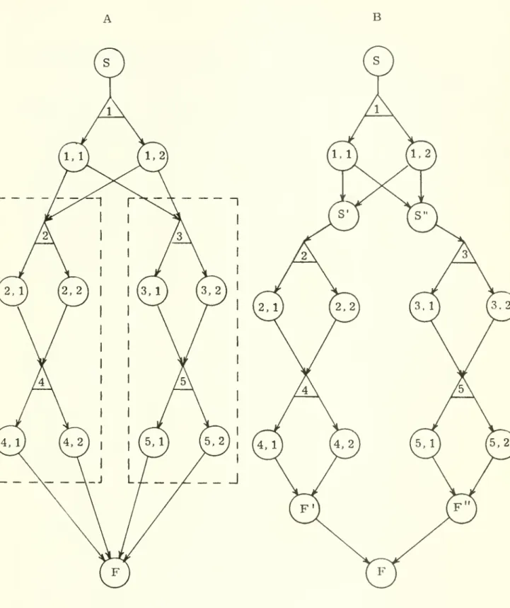
in Dantzig [3]

A

subproject is a collection of decision nodes in a reduced network

which, taken together, "look like" a project.

The

collection

must

have a

single starting point and a single finish.

There

can be no interdependency

or precedence constraint between any node within the subproject and a node which is outside the subproject.

The

starting point

may,

however, be the

successor of any

number

of jobs outside the subproject, and the finish

may

similarly

be

a predecessor of any

number

of jobs.

The

enclosed portions of the network

A

of Figure 6 qualify as subprojects.

The

network is

redrawn

as in 6B with artificial start jobs (S', S") of zero cost and time inserted, as well as artificial finish points (F', F"). In Figure 6 the following is true:

(1)

Every immediate

successor of a subproject start variable is contained by the subproject boundary.

(2)

Every immediate

predecessor of a subproject finish

variable is contained by the subproject boundary.

(3)

For

each subproject variable

which

is neither subproject start nor subproject finish, all

immediate

predecessors and successors are contained

by

the boundary.

An _{algorithm related to the network reduction}

routine of [1] has been

developed to generate all legitimate subnetworks.

-Figure 6. Decomposition of Project

Networks

-Combining

Subproject Solutions

Due

to the interaction between subprojects and the rest of the project network, it is generally not possible to solve for a single solution in each subproject and then simply to use these solutions to obtain an overall project

optimum.

A

subproject does not have, in general, its

own

objective function. Rather, the objective function is concerned with the entire project completion date; and the effect of a subproject solution

upon that date is not

known

until decisions are

made

for all other parts of

the network. Consequently,

some

other

method

of fitting subproject

solutions together in order to obtain the overall project

optimum

is needed.

The

approach is based upon the observation that the set of all feasible solutions to a subproject has all of the characteristics of a

decision node. Associated with each solution is a cost and a

performance

time, and each solution has a predecessor and a successor. In addition,

only one solution

may

be chosen

from

the subproject -- i.e. , the set of

subproject solutions is subject to a mutually exclusive interdependency constraint.

Since each solution to a subproject has the

same

predecessor and

successor (e.g., S' and F'), it is clear that the project optimal solution will never contain a subproject solution which is both longer and

more

expensive than

some

other feasible solution to the

same

subproject.

The

former

subproject solution is "dominated"

by

the latter. In the case

-23-where

a subproject solution is less expensive than

some

shorter solution,

the shorter solution is dominated if

C^

-

_C^

+

(w^

-

w^)

(max(p,r)) >

11

2 2

where

C

and w^, refer to the longer subproject solution,

C

and

w—

to the shorter, and _p and r are the overall project penalty and

premium.

In order to obtain the optimal solution to the overall project, it is

necessary to consider only all undominated solutions to each subproject.

If all undominated solutions for a subproject have

been

obtained, the entire subproject can be replaced by a single decision node containing those

solutions as its job alternatives. In the resulting

master

problem, there will be fewer decision nodes and fewer constraints.

The master problem

may

then be solved with any of the

Branch

and

Bound

routines discussed

In previous sections. Hopefully, the reduction in solution time for the

master problem

will be far greater than the time required to generate

undominated solutions to the subprojects.

The

crucial issues as to the

feasibility of this approach are: (1) the time required to generate all

\indominated solutions, and (2) the degree to which the space of all

possible subproject solutions is reduced

by dominance

considerations.

The

algorithm for determining all xindominated solutions is a

modified partitioning algorithm. Instead of a single

Z*

, there

now

exists a Z*(t) for every subproject completion time (t). Initially, Z*(t) = -»

for all t.

Obtain a first complete solution with cost

C

and completion time

(f). Then,

-24-Z*(t) =

C

for all t > t'

Z*(t) =

C

+[max

(p.r)](t' - t)

forallt<t'

When

the next complete subproject solution is obtained, the

same

calcula-tion is

made

for all t. Z*(t) is then equal to

minimum

of its current

value and the

new

calculated value.

This algorithm

was

tested on the

same

sample

of

problems

for

which

solution times are given in Table 1. It

was

found that only a small

number

of feasible undominated solutions

were

obtained (25 or less). This

is to be expected -- there can be no

more

undominated solutions than the

number

of days separating the cheapest feasible solution and the shortest.

More

surprising is that the total

amount

of time required to generate all undominated solutions is in all cases less than three times the

amount

of

time required to find the optimal solution(s).

The

conclusion that the determination of all undominated solutions will generally be at the

same

order of magnitude of difficulty as that of determining the optimal

solution

may

be

warranted.

The

partitioning algorithm, in searching for

the optimal solution,is likely to generate a

number

of complete solutions

which

it eventually determines to be bounded; but these

same

solutions

may

be undominated and thus found by the undominated solution algorithm

with very little additional effort.

To

demonstrate the

power

of the decomposition approach, two

networks

were

chosen (shown schematically in Figure 7).

The master

problem

for

Network

I includes the undominated solutions

from

subprojects

A, B, and

C

The master problem

of

Network

II includes the portion of the network

A

(not a subproject) and the undominated solutions

from

subprojects

B

and C.

-25-A

Specialized techniques for solving the master problem

may

be incorporated in a fully automated decomposition algorithm. For

example it

may

turn out that a subproject

may

always remain in the

cheapest alternative set Q, in which case it is unnecessary to gener-ate all undominated solutions for that subproject. Also, since the

predecessor-successor relationships for all undominated solutions

to a subproject are identical, the

minimum

time solution from each

subproject

may

be used to strengthen the

w

bound in the master.

There

are cases in which portions of a project network do not satisfy the strict requirements for designation as a subproject, but in

which

overall project

optimum

will be found

by

treating these portions as subprojects. Such will be the case

when

the precedence-successor

relationships which violate the subproject requirement are not on the

critical path in the optimal solution.

Or

they

may

be on the critical path,

but the undominated solutions generated in the subproject

may

be

undomi-nated regardless of the existence of the critical links. Similarly, an alternative interdependency constraint

may

cross the

boundary

but have

no effect on the optimal solution, or upon the imdominated solutions

generated

by

ignoring its existence.

The

case of the noncritical predecessor-successor link

may

often be easily seen ahead of time, so that the

decompo-sition

may

proceed with an optimal solution guaranteed. In other cases

the size of entire projects

may

be such that "illegal" decomposition

may

be

resorted to in an effort to find a good, and hopefully optimal, solution. Also, since it is true that all alternatives of a decision node need not

have identical predecessor and successor relations, it is conceivable

that algorithms could be developed for reducing a

segment

of a network

-27-to a decision node even though the

segment

does not

meet

the conditions

of an "independent subproject."

CONCLUSION

Experimentation with the algorithms discussed in this paper

shows

that

problem-

solving time

was

strongly affected by the order in which the decision nodes

were

examined. Solution time

was

miniraized

by

examining decision nodes in order of increasing "criticalness.

'

The

partitioning algorithm gave the lowest times for each

problem

tested. Its efficiency results

from

the fact that it tests each unbounded

partial solution to a

problem

to see if the cheapest alternative for each

decision node not included in the partial solution can

be

included without extending the project length. If this is the case, then all other completions

of the partial solution need not be evaluated.

The

feasibility of the

decomposition of large project networks

was

also examined. Independent

subnetworks

were

defined within a large network and these

were

solved for all undominated solutions

by

an extension of the Partitioning Algorithm.

The

set of undominated solutions can then be regarded as a simple decision

node within the large network and the resulting

problem

is solved by the partitioning algorithm described above.

The improvement

in solution

time achieved by this decomposition

was

substantial.

-28-REFERENCES

[l] Crowston,

W.

G., "Decision

Network

Planning Models",

Management

Science Research Report No.lSB, Graduate School

of Industrial Administration, Carnegie-Mellon U. , 1968.

[2] Crowston.

W.

B. , and G. L.

Thompson,

"Decision

CPM:

A

Method

of Simultaneous Planning, Scheduling, and Control of

Projects", Operations Research , Vol.15, No.3,

May-

June

1967.

[3] Dantzig, G. E., Linear

Programming

and Extensions, Princeton University Press, Princeton, N.J., 1963, Chapters 22, 23.

[4] Fulkerson, D. R., "A

Network Flow

Computation for Project Activity Scheduling",

Management

Science, Vol. 7, 1961.

[5] Kelley, J. E., Jr., "Critical Path Planning and Scheduling:

Mathematical Basis", Operations Research, Vol.7, No. 3,

1961.

[6] Lawler, E. L., and D. E.

Wood,

"Branch

and

Bound

Methods:

A

Survey", Operations Research, Vol. 14, No. 4, 1966.

[7] Parikh, S.

C,

and

W.

S. Jewell, "Decomposition of Project

Networks",

Management

Science, January 1965.

[8] Pierce, J. F., and D. J. Hatfield, "Production Sequencing

by

Combinatorial

Programming",

Operations

Research

and the

Design of

Management

Information

Systems

(J. F. Pierce, Editor),

Technical Association of the Pulp and

Paper

Industry,

New

York,

1967, p. 177.

-29-REFERENCES

(Cont.)

[9]

Wagner,

M.

H., "Solution of Decision

CPM

Networks".

S.M.

Thesis, Massachusetts Institute of Technology, June 1968.

...^,:^MM^ ,

MMSEfvlENTf

Date

Due

t'P^ \r"^ 2 19810 JUL

12

1^85 :'i\

APR

3 1^90 2 Lib-26-67

lllllliinllinliHiMi

-lO"^^

3

TD60 D03

a7M

b55

^^-Iff^

MIT LIBRARIES

I P>i| i|i|ip IIP !|iii||iii|i'ii||iiiii

3 TDflD QD3 fl7M m,s

mm