HAL Id: hal-02397154
https://hal.inria.fr/hal-02397154
Submitted on 21 Nov 2020
HAL is a multi-disciplinary open access
archive for the deposit and dissemination of sci-entific research documents, whether they are pub-lished or not. The documents may come from
L’archive ouverte pluridisciplinaire HAL, est destinée au dépôt et à la diffusion de documents scientifiques de niveau recherche, publiés ou non, émanant des établissements d’enseignement et de
Identifying the parametric occurrence of multiple steady
states for some biological networks
Russell Bradford, James Harold Davenport, Matthew England, Hassan
Errami, Vladimir Gerdt, Dima Grigoriev, Charles Hoyt, Marek Košta, Ovidiu
Radulescu, Thomas Sturm, et al.
To cite this version:
Russell Bradford, James Harold Davenport, Matthew England, Hassan Errami, Vladimir Gerdt, et al.. Identifying the parametric occurrence of multiple steady states for some biological networks. Journal of Symbolic Computation, Elsevier, 2020, 98, pp.84-119. �10.1016/j.jsc.2019.07.008�. �hal-02397154�
Identifying the Parametric Occurrence of Multiple
Steady States for some Biological Networks
R. Bradforda, J.H. Davenporta, M. Englandb,∗, H. Erramic, V. Gerdtd, D. Grigorieve, C. Hoytf, M. Koˇstag, O. Radulescuh, T. Sturmi,j, A. Weberc
aDepartment of Computer Science, University of Bath, UK
bFaculty of Engineering, Environment and Computing, Coventry University, UK cInstitute for Informatics, University of Bonn, Germany
dJoint Institute for Nuclear Research (JINR), Dubna, Russian Federation
and Friendship University of Russia (RUDN University), Moscow, Russian Federation
eCNRS & University of Lille, France
fDepartment of Life Science Informatics, B-IT, University of Bonn, Germany gSlovak Academy of Sciences, Slovakia
hDIMNP, University of Montpellier, France
iCNRS, Inria, and the University of Lorraine, Nancy, France jMPI Informatics and Saarland University, Saarbr¨ucken, Germany
Abstract
We consider a problem from biological network analysis of determining re-gions in a parameter space over which there are multiple steady states for positive real values of variables and parameters. We describe multiple ap-proaches to address the problem using tools from Symbolic Computation. We describe how progress was made to achieve semi-algebraic descriptions of the multistationarity regions of parameter space, and compare symbolic results to numerical methods.
∗Corresponding author
Email addresses: [email protected] (R. Bradford),
[email protected] (J.H. Davenport), [email protected] (M. England), [email protected] (H. Errami), [email protected] (V. Gerdt), [email protected] (D. Grigoriev), [email protected] (C. Hoyt), [email protected](M. Koˇsta), [email protected] (O. Radulescu), [email protected] (T. Sturm), [email protected] (A. Weber)
The biological networks studied are models of the mitogen-activated pro-tein kinases (MAPK) network which has already consumed considerable ef-fort using special insights into its structure of corresponding models. Our main example is a model with 11 equations in 11 variables and 19 param-eters, 3 of which are of interest for symbolic treatment. The model also imposes positivity conditions on all variables and parameters.
We apply combinations of symbolic computation methods designed for mixed equality/inequality systems, specifically virtual substitution, lazy real triangularization and cylindrical algebraic decomposition, as well as a sim-plification technique adapted from Gaussian elimination and graph theory.
We are able to determine multistationarity of our main example over a 2-dimensional parameter space. We also study a second MAPK model and a symbolic grid sampling technique which can locate such regions in 3-dimensional parameter space.
Keywords: Mixed Equation / Inequality Solving, Real Quantifier Elimination, Biological Networks, Signaling Pathways, MAPK
1. Introduction
In this work we describe the application of combinations of symbolic computation methods in various computer algebra systems to a key problem from computational biology. The work serves to demonstrate how recent advances in such algorithms, and crucially their effective combination, allows for their application on problem instances previously thought beyond reach. In this introduction we start by describing the biological networks that are our topic of study, and highlight previous relevant work. We then outline the remainder of the paper and clarify the relationship of this article to prior work.
1.1. Multistationarity
The mathematical modelling of intra-cellular biological processes has been using nonlinear ordinary differential equations since the early ages of math-ematical biophysics in the 1940s and 50s (Rashevsky, 1960). A standard modelling choice for cellular circuitry is to use chemical reactions with mass action law kinetics, leading to polynomial differential equations. Rational functions kinetics, for instance the Michaelis-Menten kinetics, can generally be decomposed into several mass action steps.
An important property of biological systems is their multistationarity by which we mean their having multiple stable steady states. It is instrumental to cellular memory and cell differentiation during development or regenera-tion of multicellular organisms and is also used by micro-organisms in survival strategies.
It is thus important to determine the parameter values for which a bio-chemical model is multistationary. As demonstrated in the next section, with mass action reactions, testing for multiple steady states boils down to count-ing real positive solutions of algebraic systems and so is suitable for study with Symbolic Computation and Computer Algebra Systems.
The models studied in this paper concern intracellular signaling pathways. These pathways transmit information about the cell environment by induc-ing cascades of protein modifications (phosphorylation) all the way from the plasma membrane via the cytosol to genes in the cell nucleus. Multistation-arity of signaling usually occurs as a result of activation of upstream signaling proteins by downstream components (Bhalla and Iyengar, 1999). A different mechanism for producing multistationarity in signaling pathways was pro-posed by Markevich et al. (2004). In this mechanism the cause of multista-tionarity are multiple phosphorylation/ dephosphorylation cycles that share enzymes. A simple, two steps phosphorylation/dephosphorylation cycle is capable of ultrasensitivity, a form of all or nothing response with no multi-ple steady states (the Goldbeter–Koshland mechanism). In multimulti-ple phos-phorylation/dephosphorylation cycles, enzyme sharing provides competitive interactions and positive feedback that ultimately leads to multistationarity (Markevich et al., 2004; Legewie et al., 2007).
1.2. Bistability
Multistationarity has important consequences on the capacity of signaling pathways to process biological signals, even in its elementary form of two stable steady states. This is known as bistability and is present in our case study problems. Bistable switches can act as memory circuits storing the information needed for later stages of processing (Weng et al., 1999). The response of bistable signaling pathways shows hysteresis, namely dynamic and static lags between input and output. Because of hysteresis one can have, at the same time, a sharp binary response and protection against chatter noise.
1.3. Prior Symbolic Work
Our study is complementary to works applying numerical methods to ordinary differential equations models used for biology applications. Gross et al. (2016a) used polynomial homotopy continuation methods for global parameter estimation of mass action models. Bifurcations and multistation-arity of signaling cascades was studied with numerical methods based on the Jacobian matrix by Zumsande and Gross (2010).
Algorithmically the task will be to count the positive real solutions of a parameterised system of polynomial or rational systems, making symbolic methods a possible tool. Due to the high computational complexity of this task (Grigoriev and Vorobjov, 1988) considerable work has been done to use specific properties of networks and to investigate the potential of multista-tionarity of a biological network out of the network structure.
This only determines whether or not there exist rate constants allowing multiple steady states, instead of coming up with a semi-algebraic descrip-tion of the range of parameters yielding this property. These approaches can be traced back to the origins of Feinberg’s Chemical Reaction Network Theory (CRNT) whose main result is that networks of deficiency 0 have a unique positive steady state for all rate constants (Feinberg, 1987; Craciun et al., 2009). We refer to Conradi et al. (2008); Mill´an and Turjanski (2015); Johnston (2014), and Conradi et al. (2017) for the use of CRNT and other graph theoretic methods to determine potential existence of multiple positive steady states, with Joshi and Shiu (2015) giving a survey.
Given a bistable mechanism it is also important to compute the bistability domains in parameter space: the parameter values for which there is more than one stable steady state. The size of bistability domains gives the spread of the hysteresis and quantifies the robustness of the switches. The work of Wang and Xia (2005) is relevant here: they used symbolic tools, including cylindrical algebraic decomposition as we do, to determine the number of steady states and their stability for several systems. They reported results up to a 5-dimensional system using specified parameter values, but their method is extensible to parametric questions. Higher-dimensional systems were studied using sign conditions on the coefficients of the characteristic polynomial of the Jacobian. In some cases these guarantee uniqueness of the steady state (Conradi and Mincheva, 2014).
1.4. Outline and New Contributions
In Section 2 we outline the particular biological model and symbolic prob-lem that we aim to solve: BioModel 26 of the MAPK network, which can be found as Model 26 in the BioModels Database of (Li et al., 2010).
In Sections 3 and 4 we describe two independent symbolic attempts to solve the problem. The first in Section 3 is able to identify symbolically the multistationarity regions of a 1-dimensional parameter space with a combi-nation of Virtual Substitution and Cylindrical Algebraic Decomposition in the Redlog package for Reduce. The second in Section 4 goes on to give full semi-algebraic solution formulae with a combination of Real Triangular-ization and Cylindrical Algebraic Decomposition using the Regular Chains Library for Maple. The solutions were obtained in different computer algebra systems using different fundamental algorithms, but all from the family of methods for real quantifier elimination. We move on in Section 5 to describe a new pre-processing method for the problems inspired by graph theory and Gaussian elimination. Then in Section 6 we describe how a combination of ideas from all three preceding sections can be combined to provide solutions over a 2-dimensional parameter space.
In Section 7 we discuss testing the stability of fixed points. Then in Section 8 we consider an alternative larger model from the MAPK network (Model 28 in the BioModels Database of (Li et al., 2010)). In Section 9 we compare the models and detour to describe a symbolic grid sampling ap-proach to this problem, including a comparison of this to a leading numerical solver. We consider how further progress could be achieved in Section 10, identifying a conjecture for determining where multistationarity for MAPK may occur without the costly calculations described. Finally we summarise and give final thoughts in Section 11.
This journal article follows published conference works at ISSAC 2017 (Bradford et al., 2017) and CASC 2017 (England et al., 2017). The present article reproduces this material clarifying, correcting and extending in places. In particular, Sections 3 and 4 were largely described in the ISSAC 2017 paper and Sections 5 and 9 in the CASC 2017 paper. The most notable new contributions are given in Section 6, where we describe for the first time semi-algebraic solutions with two free parameters; and in Section 10, where we identify a promising conjecture for future investigation.
2. Problem Outline 2.1. MAPK Bio-Model 26
The model of the MAPK cascade we are investigating can be found in the BioModels Database (Li et al., 2010) as Model 261. This is the first version of the models proposed by Markevich et al. (2004) corresponding to the so-called distributive ordered phosphorylation/dephosphorylation mechanism. Hereafter we will refer to it as Model 26.
It is given by the following set of differential equations. We have renamed the species names to x1, . . . , x11 and the rate constants to k1, . . . , k16 to facilitate reading. As usual ˙x means the time derivative of x.
˙ x1 = k2x6 + k15x11− k1x1x4− k16x1x5 ˙ x2 = k3x6 + k5x7+ k10x9+ k13x10− x2x5(k11+ k12)− k4x2x4 ˙ x3 = k6x7 + k8x8− k7x3x5 ˙ x4 = x6(k2+ k3) + x7(k5+ k6)− k1x1x4− k4x2x4 ˙ x5 = k8x8 + k10x9+ k13x10+ k15x11− x2x5(k11+ k12)− k7x3x5− k16x1x5 ˙ x6 = k1x1x4− x6(k2+ k3) ˙ x7 = k4x2x4− x7(k5+ k6) ˙ x8 = k7x3x5− x8(k8+ k9) ˙ x9 = k9x8 − k10x9+ k11x2x5 ˙ x10 = k12x2x5− x10(k13+ k14) ˙ x11 = k14x10− k15x11+ k16x1x5. (1) Later, we will use (1) to refer to (1) with all the left hand sides replaced by 0 in order to find fixed points of the system. The BioModels Database gives us meaningful values for the rate constants:
k1 = 0.02, k2 = 1, k3 = 0.01, k4 = 0.032, k5 = 1, k6 = 15, k7 = 0.045, k8 = 1, k9 = 0.092, k10= 1, k11= 0.01, k12 = 0.01,
k13= 1, k14= 0.5, k15= 0.086, k16 = 0.0011. (2)
Some of these values are accurately measured and some are well-educated guesses. For the purpose of our study we assume they are all suitable.
We may add three linear conservation constraints to this system, which in turn introduce three further constant parameters k17, k18, k19:
x5+ x8+ x9+ x10+ x11 = k17 x4+ x6+ x7 = k18
x1 + x2+ x3+ x6+ x7+ x8+ x9+ x10+ x11 = k19. (3)
Computations to produce these, for example in MathWorks SimBiology, use the left-null space of the stoichiometric matrix under positivity conditions. For details see for example Schuster and H¨ofer (1991).
The constants k17, k18, and k19 represent total initial concentrations of cell substances, and meaningful values are harder to obtain than for (2). The following are some realistic value estimates, used by Markevich et al. (2004):
k17= 100, k18 = 50, k19 ∈ [200, 500]. (4) These should be considered significantly less reliable than those in (2). In-deed, the long-term goal of our research is to treat all three of these together parametrically, although in the present work we produce results only with 0− 2 of these parameters free.
Our computational biology problem is to identify regions in (k17, k18, k19) parameter space over which the system formed by the unions of constraints in (1) and (3) under estimates (2) exhibits multistationarity.
The system has several special structure properties, e.g. it is a so called MESSI system (Mill´an and Dickenstein, 2018). However, in the following we will not directly use this structure property. The non-linearities occurring in the system are at most quadratic. As by introducing new variables the general polynomial case can be reduced to such a case and from a dynamical systems perspective point of view already quadratic systems are capable to generate all kinds of structurally stable dynamics including chaos (Vakulenko et al., 2015) this property is not restrictive.
2.2. Real Algebraic Problem
To identify fixed points we formulate a real algebraic problem by first replacing the left hand sides of all equations in (1) with 0, which as noted
above we denote (1). This, together with the equations in (3), yields an algebraic system with polynomials in
F ⊂ Z[k1, . . . , k19][x1, . . . , x11].
However, ideal theory is not sufficient, as we are concerned only with real valued solutions. Further, we have the additional inequality restrictions that all entities in our model are strictly positive. This yields an additional system
P = {k1, . . . , k19, x1, . . . , x11} ⊂ Z[k1, . . . , k19][x1, . . . , x11]
establishing a side condition on the solutions of F that all variables xi and parameters ki of P be positive. In terms of first-order logic our specification of F and P yields a quantifier-free Tarski formula,
ϕ = ^ f ∈F
f = 0∧ ^ v∈P
v > 0. (5)
The estimations for the rate constants in (2) formally establish a substitution rule σ = [0.02/k1, . . . , 0.0011/k16] in postfix notation, which can be applied to F , P , or ϕ. Applying this to ϕ; converting the floats from (2) into ra-tional numbers; and multiplying over common denominators, gives us the quantifier-free Tarski formula ψ below.
ψ =−200x1x4− 11x1x5 + 860x11+ 10000x6 = 0 ∧ −16x2x4− 10x2x5+ 500x10+ 5x6+ 500x7 + 500x9 = 0 ∧ −9x3x5+ 3000x7+ 200x8 = 0 ∧ −10x1x4− 16x2x4+ 505x6+ 8000x7 = 0 ∧ −11x1x5− 200x2x5− 450x3x5+ 10000(x8+ x9+ x10) + 860x11= 0 ∧ 2x1x4− 101x6 = 0 ∧ 4x2x4− 2000x7 = 0 ∧ 45x3x5− 1092x8 = 0 ∧ 5x2x5+ 46x8− 500x9 = 0 ∧ x2x5− 150x10= 0 ∧ 11x1x5+ 5000x10− 860x11 = 0 ∧ −k17+ x10+ x11+ x5+ x8+ x9 = 0 ∧ −k18+ x4 + x6+ x7 = 0
∧ −k19+ x1 + x10+ x11+ x2+ x3+ x6+ x7+ x8+ x9 = 0 ∧ x1 > 0∧ x2 > 0∧ x3 > 0∧ x4 > 0∧ x5 > 0
∧ x6 > 0∧ x7 > 0∧ x8 > 0∧ x9 > 0∧ x10> 0∧ x11> 0
∧ k17 > 0∧ k18 > 0∧ k19 > 0. (6) Our problem in real algebra is to obtain a semi-algebraic description of the regions in (k17, k18, k19) parameter-space where there are multiple solutions of (6). The multistationarity problem would also require to know about the stability of these solutions, as discussed in Section 7.
2.3. Suitable Symbolic Technology
This real algebraic problem is amenable to technology developed for real quantifier elimination. Note that the number of indeterminates (variables and parameters) is high compared to those usually tackled by such technol-ogy. However, the degrees involved are low, with every monomial at most degree 2, which helps make it tractable.
As we will not include a priori information about the stability of the fixed points, we must not only consider the existence of (at least) two stable fixed points but also unstable fixed points. Hence we simply investigate where in parameter space there exist multiple different roots x ∈ (0, ∞)11 of F .
In theory, any Real Quantifier Elimination (QE) technology can directly handle the parametric existence of steady states, taking as input∃x1. . .∃x11ϕ and producing as output a quantifier free formula in the parameters describ-ing where solutions exists. However, this is not sufficient to solve our problem as we are not only interested in the existence but also in the number of so-lutions. We can use a specific QE tool to do this: Cylindrical Algebraic Decomposition.
2.3.1. Cylindrical algebraic decomposition and its terminology
Cylindrical Algebraic Decomposition (CAD) was first proposed by Collins in the 1970s. This original algorithm2 took as input a set of polynomials in Z[x1, . . . , xN], producing as output a set of cells which together give a decom-position of Rn which is sign-invariant, meaning each input polynomial has constant sign over each cell. The sign-invariance means that the polynomials
may be studied over an an infinite domain by querying a finite number of sample points: one per cell.
The cells are all semi-algebraic, meaning they can be described by a poly-nomial system, and they are arranged cylindrically, meaning their projections with respect to a stated variable ordering are either equal or disjoint. The cylindricity means the semi-algebraic descriptions are triangular and the cells form cylinders over another (induced) CAD of Rn−1 given by the projection of the n-dimensional cells. All cells are either sections, defined by a poly-nomial vanishing; or a sector, defined as the space between two sections, or possibly extending infinitely.
Collins’ algorithm proceeded with a system of: projection, which identi-fied key polynomials in fewer variables; and lifting, where the induced CADs are incrementally constructed via substitution of sample points and univari-ate root isolation. The act of projection must be defined so that working at a sample point may be concluded representative for the entire cell.
There has been numerous extensions and improvements to CAD since Collins’ original method. The collection edited by Caviness and Johnson (1998) is a key resource; in particular the survey paper within by Collins (1998). A more recent survey was given in the Introduction section of the work by Bradford et al. (2016). A key choice for CAD is the variable ordering which defines the cylindricity property and controls the order steps are taken by the algorithm. For use in quantifier elimination CAD must project vari-ables in the order they are quantified. Our problem (6) is not quantified but our desire to understand the problem over parameter space means that we must project variables before parameters. However, besides this the choice is free for us. We define the main variable of a polynomial / constraint to be the highest one present (first to be projected) in the ordering.
The worst-case time complexity of CAD is doubly exponential. Tradi-tionally, this is doubly exponential in the number of indeterminates, which would include our symbolically treated parameters. However recent progress on CAD in the presence of equational constraints (see for example the work of England et al. (2015)), of which there are many in (6), allows us to con-clude it is actually doubly-exponential in the number of variables minus the number of equational constraints at different levels of the projection (Eng-land and Davenport, 2016). Despite this, the number of variables present in (6) is too large for contemporary CAD implementations to tackle alone.
2.3.2. Combing with other symbolic tools
We are able to make progress by combining CAD with additional sym-bolic methods. Two independent investigations were undertaken. The first, described in Section 3, uses the Redlog package in Reduce and combines CAD with virtual substitution. The second, described in Section 4, uses the Regular Chains Library in Maple and combines CAD with real triangulariza-tion. In both cases we have combined the corresponding methods by hand, but automation is clearly possible.
3. Using Real Quantifier Elimination Technology in Redlog
In this section we are going to combine Virtual Substitution (VS) with CAD. The former smoothly eliminates the majority of the quantifiers while the latter allows us to count numbers of solutions via decomposition of the remaining low-dimensional spaces. That combination of methods requires the solution of several QE runs with each problem and some combinatorial arguments. Throughout this section we are performing computations using the Redlog Package (Dolzmann and Sturm, 1997a) for Reduce revision r3606. Timings are reported for a 2.4 GHz Intel Core i7 with 3 GB RAM or cores on a compute server with similar speed and memory limitations.
3.1. Virtual Substitution
Substitution methods for quantifier elimination date back to an article from Weispfenning (1988), which treated the special case with only linear occurrences of the quantified variables. Originally motivated by the proof of tight complexity bounds for the real decision problem, that approach turned out to be applicable to practical problems, especially with many parameters. Consequently, the method was systematically generalized by Weispfenning and his students to arbitrary but bounded degrees (Weispfenning, 1997b, 1994; Koˇsta, 2016).
Quantifier elimination proceeds from the inside to the outside of a prenex quantifier block. An innermost existential quantifier is eliminated by equiv-alently replacing it with a finite disjunction:
VS(∃xnϕ) := _ t∈E
ϕ[t//xn],
where E is a finite elimination set containing abstract test points t = (γ, z). The terms z are derived from symbolic representations of formal zeros of
parametric univariate polynomials from Z[x1, . . . , xn−1][xn] occurring in ϕ with possibly adding infinitesimals ±ε. They are guarded by quantifier-free formulas γ(x1, . . . , xn−1) that guarantee the existence of the zeros in terms of the parameters. Recall that regular term substitution maps terms to terms, which naturally generalizes to corresponding maps on quantifier-free formulas. Virtual substitution [t//xn], in contrast, maps atomic formulas to quantifier-free formulas. This allows to express the substitution of the terms z without using any non-standard symbols. Furthermore, virtual substitution adds the guarding conditions γ in a suitable way. For examples and surveys of the virtual substitution method see the work of Sturm (2017, 2018). 3.2. Parameter Free Computations
We start by considering the case where all parameters in (5) are substi-tuted for their estimates in (2) and (4) (interpreted as rational numbers):
ϕ500 = ϕσ[100/k17, 50/k18, 500/k19].
The closed formula ¯ϕ500 =∃x1. . .∃x11ϕ500 states the existence of a suitable real solution. In a first step, we solve for i∈ {1, . . . , 11} the following eleven QE problems using VS:
ϕ(i)500 = VS(∃x1. . .∃xi−1∃xi+1. . .∃x11ϕ500).
Each ϕ(i)500 is a univariate quantifier-free formula describing all possible real choices for xifor which there exist real choices for all other variables such that ϕ500 holds. CAD can easily decompose the corresponding one-dimensional spaces. It happens that for each xi there are exactly three zero-dimensional cells ai, bi, ci ∈ R where ϕ
(i)
500 holds. We extract all ai, bi, and ci as real algebraic numbers, i.e., as the unique root of a univariate defining polyno-mials with integer coefficients within an isolating interval. By combinatorial arguments it is not hard to see that the following holds for the set S500 of real solutions of ϕ500: 3≤ |S500| and S500 ⊆ 11 Y i=1 {ai, bi, ci}.
Notice that at this point we have proven the existence of multiple fixed points of the system for k19 = 500. We can furthermore compute S500 by plugging the 311 candidates from the Cartesian product into ϕ
Table 1: The unique solution x(200) for k
19 = 200 and the three solutions x(500)1 , x (500)
2 ,
x(500)3 for k19= 500. Note that we have actually computed real algebraic numbers, which
are pairs of univariate polynomials and isolated intervals. For convenience we are giving machine float approximations here, which can be made arbitrarily precise.
x(200) x(500)1 x(500)2 x(500)3 x1 90.6512 17.6392 122.034 323.761 x2 2.67311 6.97675 14.6721 9.49621 x3 10.4996 367.57 234.974 37.1013 x4 17.8545 36.6772 14.5102 6.72938 x5 35.9695 5.50874 7.16952 13.6295 x6 32.0501 12.811 35.064 43.1428 x7 0.0954536 0.511775 0.42579 0.127807 x8 15.5631 83.4416 69.4223 20.8381 x9 2.39331 8.06095 7.43877 3.21139 x10 0.641001 0.25622 0.70128 0.862856 x11 45.4331 2.73253 15.2681 61.4581
approach requires arithmetic with real algebraic numbers followed by the determination of the signs of the results, which is quite inefficient in practice. However, it turns out that interval arithmetic starting with refinements of the isolating intervals of the real algebraic numbers excludes 311− 3 of the candidate solutions. Even the three remaining candidates then require no further checking with algebraic numbers since we already know that |S500| ≥ 3. The overall CPU time is 71.3 seconds for 11 runs of VS plus 11 runs of CAD, followed by 16 hours for checking candidates. Our checking procedure is a file-based prototype starting a Reduce process for every single of the 311 candidates; there is considerable room for optimization.
For k19= 200 instead of 500 all eleven univariate CAD computations yield unique solutions which can be straightforwardly combined to one unique so-lution for the corresponding ϕ200. The overall CPU time here is 66.4 seconds for 11 runs of VS plus 11 runs of CAD. Machine float approximations of all our solutions are given in Table 1.
3.3. Parametric Analysis for k19
We next consider the case where k19 is left as a free parameter:
ϕk19 = ϕσ[100/k17, 50/k18]. (7)
Again, we solve for i∈ {1, . . . , 11} eleven QE problems using VS: ϕ(i)k
19 = VS(∃x1. . .∃xi−1∃xi+1. . .∃x11ϕk19).
This time each ϕ(i)k
19 is a bivariate quantifier-free formula in k19 and the
corre-sponding xi. Hence we must now construct a two-dimensional CAD for each ϕ(i)k
19. The projection order is important: we first project xi, then the CAD
base phase decomposes the k19-axis, followed by an extension phase that de-composes the xi-space over the k19-cells obtained in the base phase. This is feasible if we make one limitation: not to extend over zero-dimensional k19-cells. In other words, we accept finitely many blind spots in parameter space, which we can explicitly read off from the CAD so that in the end we know exactly what we are missing.
Figure 1 shows our CAD tree for ϕ(2)k
19. The first layer from the root shows
the decomposition of the k19-axis. The five zero-dimensional (rectangular) cells are the previously mentioned blind spots, among which the smallest one is not relevant, as it has negative value of k19. Those zero-dimensional cells also establish the limits of the full dimensional (oval) cells in between. The cylinders over those one-dimensional k19-cells each contain either one or three zero-dimensional x2-cells where ϕ
(2)
k19 holds. We have deleted from the
tree all x2-cells where ϕ (2)
k19 does not hold.
We make two observations, important for a qualitative analysis of our system:
(i) For all positive choices of k19, extending to infinity, there is at least one positive solution for x2.
(ii) There is a break point around k19= 409.253 where the system changes from having a unique solution to exactly three solutions.
Recall that for all floating point numbers given here as approximations we in fact know exact real algebraic numbers. For instance, the exact break point is the only real zero in the open interval (409, 410) of an irreducible defining polynomial
10 X
i=0
Figure 1: The pr uned CAD tree for x2 . Ellipses and rectangles are full-dimensional and zero-dimensional ce lls , resp ectiv ely . W e ha ve remo ved cells where k19 is negativ e or where the input form ula is false.
Figure 2 depicts all eleven CAD trees for ψk(1)
19, . . . , ψ
(11)
k19 . They are quite
similar to the one just discussed. Even the break point from one to three solutions for xi is identical for all i ∈ {1, . . . , 11} so that we can generalize our observations from earlier:
(i) For all positive choices of k19, extending to infinity, there is at least one positive solution for (x1, . . . , x11).
(ii) There is a break point β around k19= 409.253 where the system changes its qualitative behaviour. We have exactly given β as a real algebraic number in Equation (8). For k19 < β there is exactly one positive solution for (x1, . . . , x11). For k19 > β there are at least 3 and at most 311 positive solutions for (x
1, . . . , x11).
The overall computation time for our parametric analysis is 4.3 minutes. It is strongly dominated by 2.8 minutes for the computation of one particular CAD tree, for ϕ(11)k
19 . It turns out that the suitable projection order with xi
eliminated first is computationally considerably harder than projecting the other way round. As a preprocessing step we apply CAD-based simplification of the ϕ(i)k
19 with the opposite, faster, projection order. Here we use
QEPCAD-B (v1.69), which performs better than Redlog at simple solution formula construction (Brown, 2003).
4. Using Triangular Decomposition Tools in the Regular Chains Library for Maple
In this section we are going to apply triangular decomposition methods, including CAD. We find that a triangular decomposition can derive solution formulae for many variables in terms of a smaller subset for which we must apply CAD to count solutions. Throughout this section we are performing computations in Maple 2016, but using an updated version of the Regular Chains Library3. Timings are reported for a Windows 7 64 bit Desktop PC with Intel i5.
4.1. Parametric Analysis for k19
Regular chains are the triangular decompositions of systems of polynomial equations, where triangular means decreasing subsets of variables occurring
Figure 2: All CAD trees for ψ(1)k19, . . . , ψ (11)
k19 . In the second but last row on the left hand
side there is the tree for ψ(1)k19, which is displayed in detail in Figure 1. Note that in the
digital version of this article readers can zoom into these trees to see the details (as are visible in the printed version of Figure 1).
in each polynomial. Highly efficient methods for working in complex space have been developed based on these; see the work of Wang (2000) and Aubry et al. (1999) for a survey.
Recent work by Chen et al. (2013) proposes adaptations of these tools to the real analogue: semi-algebraic systems. They describe two algorithms to decompose any real polynomial system into finitely many regular semi-algebraic systems. The first, Real Triangularize (RT), does so directly while the second, Lazy Real Triangularize (LRT), produces the highest (complex) dimension solution component and unevaluated function calls, which if all evaluated would combine to give the full solution. These algorithms are implemented in the Regular Chains Library for Maple.
We will apply LRT on the quantifier-free formula (5) evaluated with the parameter estimates for k1, . . . , k18, i.e. the system (7) as studied with Redlog in Section 3.3.
We need to choose a variable ordering: our analysis requires that k19 be the indeterminate considered alone. We place the remaining variables in lexicographical order since the in-built heuristics to make the choice could suggest nothing better. The solutions must hence contain constraints in k19, constraints in (x1, k19), in (x2, x1, k19) and so on.
Applying LRT this way produces one solution component and 6 uneval-uated function calls in around 15 seconds.
4.1.1. The main solution component from LRT
In the evaluated component: for each of x2, . . . , x11 there is a single equation which has this as the main variable. Further, these are all linear in their main variable meaning they can be easily rearranged into the solution formulae given below.
x11 =− 1 60x 2 2+ 1 600(10k19− 10x1− 37x3+ 10x4 − 2100)x2− 9 200x 2 3 + 1 600(−27x1+ 27x4+ 27k19− 4650)x3− x1+ x4+ k19− 50 (9) x10 = 1 150x2(x2+ x3− x4− k19+ x1+ 150) (10) x9 = 1 18200(69x3+ 182x2)(x2+ x3− x4− k19+ x1+ 150) (11) x8 = 15 364(x2+ x3− x4− k19+ x1+ 150)x3 (12)
x7 = 50− 2 101x4x1− x4 (13) x6 = 2 101x4x1 (14) x5 = x2 + x3− x4− k19+ x1+ 150 (15) x4 = 2525000/(101x2+ 1000x1+ 50500) (16) x3 = n3/d3 where (17) n3 =−101x32− (−101k19+ 1101x1+ 65650)x22− (1000x21 + (−1000k19+ 200500)x1− 50500k19+ 5050000)x2+ 150000x1) d3 = 101x22+ (1000x1+ 50500)x2 x2 = n2/d2 where (18) n2 = 30625833064790009548991419920x51 + (−43795148662369306906962603840k19 + 37749979225487731805273686504663200)x41 + (14871210647782462053693235920k192 − 16963336293692750919154910690672400k19 + 6815925407229297763234036009365120000)x31 + (1538325448222983229930530049200k219 − 862702164104208291031357996000020000k19 + 279241219028720368578809336249748000000)x21 + (29370341694954648101085099000000k219 − 12995812279808313524592161760000000k19 + 3705960282117523242886769213700000000000)x1 − 126235874510278395777369000000000000k19 d2 = 232763663752113237974029404420089x51 + (−332853615301041845577671639990228k19 + 88646303215205075376308147029677220)x41 + (113024761399450186949390623074789k192 − 80843908028331498139954527761762740k19 + 11682465068391769796632986929072776500)x31 + (11455232309649034305597048791479020k219 − 5547251026060433566640620528023877000k19
+ 619147207587597001268026254404647600000)x21 + (290245997063001550130198026458525000k219 − 141348286758352762323489548674398500000k19 + 14547288529581382252587071541494600000000)x1
− 1247498501818579946626756931775000000000(k19− 100) Note that these solution formula: are guaranteed valid for all positive k19 excluding three isolated points which are provided as part of the output from LRT and described below; are triangular, with each xk is expressed in variables {xi, i < k}; and are provided for all but variable x1.
The output of LRT also requires that x1 be both positive and satisfy:
f (x1, k19) = 6 X
i=0
dixi1 = 0 (19)
where the coefficients diare univariate polynomials in k19of maximum degree 2 as given in Appendix B. Hence there are at most six solutions for x1, with the exact number depending on whether solutions of (19) are real and positive.
There are four constraints on free parameter k19 as given below, one of which is the non-vanishing of the polynomial in Appendix Appendix A whose root defined the break point found by Redlog in Section 3.3. Note that the coefficients break over lines within the final constraint.
k19> 0 (20) ∧ polynomial in (8) 6= 0 (21) ∧ 23197989433419579994929k2 19− 89407400615452409453098800k19 − 4822419303419166525491149190000 6= 0 (22) ∧ 505465566622475867655547880786544637953790406059982726185509k4 19 − 1272578045696439189317856051518387368422217896986836692050 5134120k319+ 117551033091520524183124321323141751700303731556 2884193657451445400k192 − 281867359883676159811192082978541193 600292804324596911878337972560000k19− 42434363570215587465 6684237015639321850510668927412079318793072000000006= 0 (23) Evaluating the real roots of the polynomials appearing in the above allows us to conclude that this solution component is valid for all positive values
of k19 excluding three points. As with Redlog, Maple can represent these as exact algebraic numbers but for brevity we give float approximations:
409.253, 16473.337, and 25084.536. (24)
Software Remark 1. In the authors’ ISSAC 2017 paper (Bradford et al., 2017) the description of the evaluated solution component ended here. How-ever, following the publication of that paper a bug was uncovered by one of the authors in the simplifier of the Regular Chains Library when working with a different MAPK model to the one considered presently. For that ex-ample the simplifier was incorrectly discarding certain positivity conditions. The bug was reported to the Regular Chains developers, and the current version of the simplifier4 now excludes all such simplifications. So presently, the output from LRT includes also the positivity conditions
x2 > 0, x3 > 0, . . . , x11 > 0.
Some of these can clearly be removed. For example, if we know x1 > 0 and x2 > 0 then (16) implies x4 > 0 and this coupled with (14) implies x6 > 0. However, it is not trivial to imply all such inequalities, and so any proposed solution in (k19, x1) should be checked to see if it implies a positive solution in all the remaining variables before being accepted. This is indeed the case for all solutions described in the ISSAC 2017 paper, and below.
4.1.2. The unevaluated function calls from LRT
The main solution component described in Section 4.1.1 is not the entire solution to the system. LRT produced also six unevaluated function calls which if evaluated and combined with the main component would give the full solution. LRT guarantees that the complex dimension of the solution components from these unevaluated calls is smaller that the main component. In fact, three of the six unevaluated calls define empty solution sets, with evaluating to discover this instantaneous.
With regards to the other three: we can infer from the arguments to these function calls that each defines the solution at one of the three points in (24) that were excluded from the main component. I.e. each of these three calls has as an argument the negation of one of the univariate inequations
4
for k19from (21)−(23). Actually evaluating these solution components is not possible in reasonable time. Thus, as with Redlog in Section 3, we proceed accepting a small number of blind spots.
The output of LRT has quickly given us the structure of the solution space valid at all but three isolated values of k19. However, it does not identify where the number of real solutions change. Note that although the break point identified in Section 3 has been rediscovered in (24), there is not yet any information gathered by Maple from which we can infer its significance. We also note that there seems to be no significance for our application of the other two isolated points in (24).
4.1.3. Counting solutions with CAD
To finish the analysis we need to decompose (x1, k19)-space according to the real roots of f (x1, k19); and also x1 and k19 since the constraints x1 > 0 and k19 > 0 were specified separately in the output. CAD is ideally suited for this task. We apply the Regular Chains based implementation in Maple first described by Chen et al. (2009). A CAD for f (x1, k19), with the ordering chosen so that the k19-axis is the one decomposed, divides the plane into 135 cells in a few seconds. This CAD decomposes the k19 axis into 11 cells, i.e. identifying five points, which approximate to:
−379.993, −87.776, 0, 409.253, and 25084.536.
We give these as floats for brevity but exact algebraic numbers are available5. On the cell where 0 < k19 < 409.253, the cylinder above in the (x1, k19)-plane is divided into 11 cells: three of which cover x1 > 0 (two 2d sectors and a 1d section). We see that f (x1, k19) is zero on the section but not the sectors. This can be inferred by testing a sample point of the section (the invariance properties of the CAD mean that the signs of the input at this point are representative for the whole cell. In fact, with the CAD implementation we use the cells comes with a semi-algebraic description which for this section is the statement that f (x1, k19) = 0 (along with the bounds on k19).
We can perform a similar analysis on the two cells for 409.253 < k19 < 25084.536 and 25084.536 < k19 < ∞. In each case the cylinders above are divided into 15 cells, seven of which cover x1 > 0, with the three sections satisfying f (x1, k19) = 0.
So we can conclude that: (a) if 0 < k19 < 409.253 then f (x1, k19) has a single positive real solution; and (b) if k19 ∈ (409.253, ∞) \ {25084.536} then f (x1, k19) has three positive real solutions. We cannot conclude with certainty what happens at the points 409.253 and 25084.536.
At the end of this analysis we have rediscovered the break point identified in Section 3 where the system moves from a single positive real solution to three. We also have explicit solutions valid for all except three isolated k19 values. To obtain an actual numerical solution we need only: select the k19 value of interest (call it ˆk19); perform univariate root isolation on f (x1, ˆk19), noting we know in advance how many to expect based on ˆk19; then for each x1 solution substitute recursively into equations (9)−(18), starting with (18) and working up, substituting the new variable solution from each formula into the next. The solutions in Table 1 may be easily rediscovered this way, for example.
We note that, as discussed in Software Remark 1, we have ensured that for each cell all the positive solutions in x1 provided by the sample point do indeed lead to positive solutions for all other variables via the back substi-tution process.
4.2. Repeating for Other Choices
We have repeated the approach described in Section 4.1 for different choices of free parameter and different choices of fixed parameter values. For example:
• With k17 set to 95 instead of 100 we find that the break point between 1 and 3 real positive solutions moves to k19 = 369.917. With k17 set to 105 it moves to k19= 450.077.
• Allowing k17 to be free and fixing k19 = 200 we find that there is only ever one positive real solution.
• Allowing k17 to be free and fixing k19 = 500 we find the number of positive real solutions moving from 1 to 3 to 1 breaking at k17 = 85.988 and k17 = 110.869.
• Similarly, allowing k18 to be free and fixing k19 = 200 we find there is only ever one positive real solution; but fixing k19 = 500 instead we find 3 real solutions between k18= 44.434 and 58.329 and 1 otherwise.
This hints that there is a shape approximating a paraboloid within (k17, k18, k19)-space within which bistability may occur; with bistability available for any k17 and k18 value but bounded from below in the k19 coordinate.
We note that these conclusions are, as with the one described in detail, valid at all but a handful of isolated values of the free parameter.
5. A Graph Theory Guided Parametric Gaussian Elimination Pre-processing Method
As described above, the complexity of polynomial systems obtained with steady-state approximations of biological models is comparatively high for the application of symbolic methods, particularly in reference to the dimen-sion (number of indeterminates). The two studies described in Sections 3 and 4 both used tools to effectively reduce the problem dimension before applying the costly CAD method.
More generally, it is highly relevant for the the success of general polyno-mial systems methods if we can first identify and exploit particular structural properties of the input. Here, the MAPK models have remarkably low total degrees with many linear monomials after some substitutions for rate con-stants. For example, the final equation of (1) suggests a simple polynomial expression for x11 in terms of the remaining variables of the system. This promoted the idea of pre-processing MAPK input with essentially Gaussian elimination: in the sense of solving single suitable equations with respect to some variable and substituting the corresponding solution into the system. 5.1. Parametric Gaussian Elimination
Generalizing this idea to situations where linear variables have parametric coefficients in the other variables requires, in general, a parametric variant of Gaussian elimination, which replaces the input system with a finite case dis-tinction with respect to the vanishing of certain coefficients and one reduced system for each case. Further, for our problem the positivity conditions establish a further apparent obstacle, because we are formally not dealing with a parametric system of linear equations but with a parametric linear programming problem.
The theory of real quantifier elimination by virtual substitution tells us that it is sufficient for the inequality constraints to play a passive role in the sense that their polynomials do not contribute to the elimination set E discussed in Section 3.1. This key idea occurred first for the linear case
in Theorem 3.11 of the work by Loos and Weispfenning (1993); while the current state-of-the-art is described in the thesis of Koˇsta (2016). The crucial observation is that our entire formula is (and remains during the considered elimination) a single Gauss Prime Constituent in the sense of (Koˇsta, 2016, Section 3.1.1). Further, for the considered MAPK model, it turns out that those positivity assumptions on the variables are actually strong enough to guarantee the non-vanishing of all relevant coefficients, so case-distinctions are never necessary! We do not claim such an approach will always be so lucky, but it may be this result generalises for the MAPK hierarchy. It was the case also for the second larger MAPK model we describe in Section 8. 5.2. An Optimal Strategy
Parametric Gaussian elimination can increase the degrees of variables in the parametric coefficient, in particular destroying their linearity and suit-ability to be used for further reductions. For example, solving the last equa-tion of (1) and substituting into the first equaequa-tion would destroy any linearity present in that first equation.
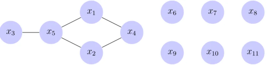
The natural question is whether there is an optimal strategy to Gauss-eliminate a maximal number of variables? This has been answered positively only recently by Grigoriev et al. (2015): draw a graph, where vertices are variables and edges indicate multiplication between variables within some monomial. Then one can Gauss-eliminate a maximum independent set, which is the complement of a minimum vertex cover. Figure 3 shows that graph for (1), where {x4, x5} is a minimal vertex cover, and all other variables can be linearly eliminated.
Recall that minimum vertex cover is one of 21 classical NP-complete prob-lems described by Karp (1972). However, our instances considered here and instances to be expected from other biological models are so small that the use of existing approximation algorithms (Grandoni et al., 2008) appears un-necessary. We have used real quantifier elimination, which did not consume measurable CPU time; alternatively one could use integer linear program-ming or SAT-solving.
It is a most remarkable fact that a significant number of biological mod-els in the databases have that property of loosely connected variables. This phenomenon resembles the well-known community structure of propositional satisfiability problems, which has been identified as one of the key struc-tural reasons for the impressive success of state-of-the-art CDCL-based SAT solvers by Girvan and Newman (2002).
x3 x5 x1 x2 x4 x6 x7 x8 x9 x10 x11
Figure 3: The graph for (1) is loosely connected. Its minimum vertex cover {x4, x5} is
small. All other variables form a maximum independent set, which can be eliminated with linear methods.
5.3. Reduced System for Model 26
We conclude this section with the reduced system computed with an im-plementation of this pre-processing in Redlog (Dolzmann and Sturm, 1997a). From (6) we obtain ψ = x5 > 0 ∧ x4 > 0 ∧ k19> 0 ∧ k18> 0 ∧ k17> 0 ∧ 1062444k18x24x5+ 23478000k18x24+ 1153450k18x4x25+ 2967000k18x4x5 + 638825k18x35+ 49944500k18x25− 5934k19x24x5− 989000k19x4x25 − 1062444x3 4x5− 23478000x34− 1153450x 2 4x 2 5− 2967000x 2 4x5 − 638825x4x35− 49944500x4x25 = 0 ∧ 1062444k17x24x5+ 23478000k17x24+ 1153450k17x4x25+ 2967000k17x4x5 + 638825k17x35+ 49944500k17x25− 1056510k19x24x5− 164450k19x4x25 − 638825k19x35− 1062444x 2 4x 2 5− 23478000x 2 4x5− 1153450x4x35 − 2967000x4x25− 638825x 4 5− 49944500x 3 5 = 0. (25)
We now have a system of just two equalities in 5 indeterminates together with positivity conditions on those indeterminates. Notice that no compli-cated positivity constraints come into existence from this method. All cor-responding substitution results are entailed by the other constraints, which is implicitly discovered by using the standard simplifier of Dolzmann and Sturm (1997b) during preprocessing.
Note that, with ψ defined in (6), we have a formal equivalence here, from the theory of quantifier elimination via virtual substitution:
∃x1∃x2. . .∃x11ψ =∃x4∃x5ψ.
So if we can determine the region of parameter space where solutions to ψ exist we are guaranteed to also find solutions to ψ there. However, our
problem concerns not just the existence of solutions but the number, and so on the surface this may seems inadequate. However, because the only technology used in this reduction is linear substitution we can also conclude that the number of solutions found for ψ will lead to the same number of solution of ψ.
Hence it is sufficient to study ψ. This pre-processing allows us to derive solutions with two free-parameters in the next section. We also give some indication of the performance improvements of various methods offered by the pre-processing later in Section 9.
6. Combined Approach for a Solution over 2-parameter space In this section we describe a new derivation of a solution to the real algebraic problem with two free parameters, produced after the publication of the authors’ ISSAC 2017 and CASC 2017 conference papers (Bradford et al., 2017; England et al., 2017). The progress is made by combining ideas from all three of the preceding sections. We describe in detail below but broadly we: start with the reduced system from the pre-processing of Section 5 with two free-parameters; apply the LRT method of Section 4 to reduce the problem by an indeterminate; build part of a CAD, an idea used in Section 3, sufficient to identify the regions of parameter space of interest. Timings are reported for the same hardware and software as Section 4.
6.1. Applying LRT and Preparing for CAD
We start with the reduced system (25) derived in Section 5 above. We set k18 to 50 and leave k17 and k19 free. Hence we seek the regions of the (k17, k19)-plane where there exist multiple solutions.
We first run the LRT algorithm introduced in Section 4, using variable ordering (x4, x5, k17, k19). We needed the parameters to come after the vari-ables so we work over the parameter space, but within the pairs the orders could have been reversed. In around 5 seconds LRT outputs one solution component and 4 unevaluated function calls.
The evaluated component consists of the four positivity conditions from the input and the two equations, which may be seen in Appendix C where they are labelled (C.1) and (C.2). Of course these equations are triangular: (C.1) involves {x4, x5, k17, k19} while (C.2) does not depend on x4. Note that (C.1) is linear in x4 and so we can easily rearrange to give a solution formula for x4 in terms of (x5, k17, k19). (C.2) is of degree 6 in x5 but of course not all
its solutions need be real and positive. If we can determine where (C.2) has multiple positive real solutions then all that remains is to back substitute and to get real solutions for the other variables and check these are also positive. We will determine this using CAD.
Before that, we examine the 4 unevaluated functions calls from LRT: two instantaneously evaluate to empty solution sets while the other two cannot be evaluated in reasonable time. We infer from the arguments to the function calls that the latter two define solutions on the graphs of two polynomials in (k17, k19)-space. These two polynomials may be found in Appendix D. The smaller is degree 5 in k17 and degree 4 in k19 (total degree 5 overall) and the larger degree 14 in k17 and degree 10 in k19 (total degree 14 overall)6.
We proceed on the understanding that any results are valid everywhere in (k17, k19)-space except on these graphs. We may compare this to Sections 3.3 and 4.1 which accepted a finite number of isolated blind spots in a one-dimensional parameter space.
6.2. Solution via an Open CAD
A CAD sign-invariant for the polynomial defining (C.2) (and x5, k17, k19 to allow for positivity checks) would be sufficient. However, the size of the polynomial puts this beyond CAD currently. Instead, we proceed as follows: Step 1: Calculate the projection set for CAD input consisting of polynomial
defining (C.2) and polynomial x5 (to allow for positivity check). This is a set of 19 polynomials in (k17, k19) the greatest of which has degree 34, and so it is not reasonable to print them all here.
Step 2: Build an Open CAD of (k17, k19)-space for these polynomials, along with polynomials k17 and k19 (to allow for positivity checks).
An Open CAD means the full dimensional cells only. The boundaries may be determined by algebraic numbers but because we do not lift over the bound-aries there no costly algebraic number calculations. The idea has been much discussed by McCallum (1993); Strzebo´nski (2000); Wilson et al. (2014), and other names used for it include generic CAD and 1-layered Sub-CAD. It was
6As described later in Section 10.3 the boundary of the multistationarity region is
actually defined by part of the graph of one of these polynomials, although there is no reason to conclude that at this stage of the analysis.
partly applied by the approach in Redlog in Section 3. It is sufficient to solve problems which are only in strict inequalities, but of course, that is not the case here. By making this restriction we are accepting that our solutions and conclusions are not necessarily valid on cell boundaries: a finite number of curve segments in the (k17, k19)-plane. However, we have already made such an acceptance, in the use of LRT above.
We perform the above steps with the ProjectionCAD package of England et al. (2014) in Maple7 in 17 seconds. The resulting CAD has 533 cells. Step 3: Identify those cells in the upper quadrant of the (k17, k19)-plane. We only care about solutions in this upper quadrant. We can easily identify 139 such cells by querying sample points (note that no cell can straddle the boundary of the quadrant since the CAD produced was also produced sign-invariant for k17 and k19 as polynomials). Since in Step 1 we ensured that this CAD was built for the projection of the polynomial defining (C.2) we may conclude that for this polynomial we can work at a sample point of the cell but draw conclusions for the whole cell, as we do next.
Step 4: Identify the number of positive real roots the polynomial defining (C.2) has over each of these cells.
We do this by substituting for the sample point and applying Maple’s default real root isolation algorithm. We identify 35 of the 139 cells where there are three positive real roots for x5, with the other 104 all having one. Step 5: Check that these solutions provide a positive solution for x4 via
back substitution into (C.1).
We first checked that the 104 cells with one positive real solution for x5 all lead to one positive real solution for x4 as expected. We then analyse the 35 cells and each of their three positive real solutions for x5 in turn. For 28 of these cells each solution gives a corresponding positive real solution for x4. For the other 7 cells, only one of the three solutions does, so these join the other 104 as representing the parameter space with one solution.
The semi-algebraic descriptions of these 28 cells provide the exact de-scription of the regions in (k17, k19)-space where multistationarity can occur.
7
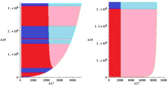
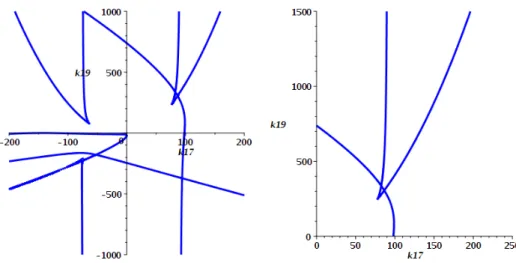
We use these descriptions to produce the 4 plots of the multistationarity region in Figures 4 and 5. The 4 images are all produced from the data in the 28 cells, but with different plotting regions. In each case, the coloured regions represent the cells with multistationarity, with the only purpose of the different colours to show the separation of the cells8.
The left plot in Figure 4 is for the original range of k19 values considered and has the region of multistationarity described by 4 full dimensional CAD cells. The right plot shows that this region grows as k19 increases: at this range 9 cells are in view including the 4 from the left plot which are at the bottom of the region.
The left plot of Figure 5 expands the ranges considerably. There are 24 cells in view of the range but the original 9 described above are now too small to see. The right plot of Figure 5 expands the range further to include all 28 cells; with all 24 from the previous image now too small to see. In this final image the two cells at the top actually extend infinitely in the k19 direction while always being bounded on both sides in the k17 direction.
7. Stability of Fixed Points
The work described in Section 3−6 was dedicated to identifying where multiple fixed points occur. This alone does not prove multistationarity as we must also check the stability properties of these fixed points.
We may use the three linear conservation constraint equations (3) to eliminate x1, x7, and x11 from system (1) and symbolically compute the Ja-cobian ˜J of the obtained reduced system. We can then numerically compute the eigenvalues of ˜J for the instances arising from the substitution of the parameter values and the different positive fixed points for the variables.
We have used the float approximations for the unique solution x(200) with k19 = 200 and the three solutions x
(500)
1 , . . . , x (500)
3 for k19 = 500 in Table 1. For the single positive fixed point x(200)the Jacobian ˜J (x(200)) has eigenvalues with negative real part only and hence can be shown to be stable. For k19 = 500 one of the three positive fixed points x
(500)
2 can be shown to be unstable, as ˜J (x(500)2 ) has one eigenvalue with positive real part; the other seven had negative real parts. In contrast x(500)1 and x(500)3 can be shown to be stable. Hence for k19= 500 the system is indeed bistable.
8Because we produced an Open CAD above we cannot formally conclude what happens
Figure 4: Visualisations of the Open CAD cells describing the multistationarity region derived in Section 6 for smaller values of k17and k19.
Figure 5: Visualisations of the Open CAD cells describing the multistationarity region derived in Section 6 for larger values of k17 and k19.
A verification of the stability of the fixed points using exact real algebraic numbers by the well-known Routh–Hurwitz criterion is possible algorithmi-cally (Hong et al., 1997), but seems to be out of range of current methods for this example. Notice that in other studies on multistationarity of signaling pathways, such as those of Conradi et al. (2008) and Gross et al. (2016b), the question of stability has also been left to one side.
8. Another MAPK Model
We describe a second MAPK model, which we will use alongside the first from Section 2 in the remaining sections, to broaden the conclusions drawn. 8.1. MAPK Bio-Model 28
The system with number 28 in the BioModels Database is given by the following set of differential equations. This model is the distributive fully random kinetics version of the models proposed by Markevich et al. (2004). Hereafter we refer to it as Model 28. Again, we have renamed the species to x1, . . . , x16 and the rate constants to k1, . . . , k27 to facilitate reading:
˙x1 = k2x9+ k8x10+ k21x15+ k26x16 −k1x1x5 − k7x1x5− k22x1x6− k27x1x6 ˙x2 = k3x9+ k5x7+ k24x12− k4x2x5− k23x2x6 ˙x3 = k9x10+ k11x8+ k16x13+ k19x14− k10x3x5− k17x3x6− k18x3x6 ˙x4 = k6x7+ k12x8+ k14x11− k13x4x6 ˙x5 = k2x9+ k3x9+ k5x7+ k6x7+ k8x10+ k9x10+ k11x8+ k12x8− k1x1x5− k4x2x5− k7x1x5− k10x3x5 ˙x6 = k14x11+ k16x13+ k19x14+ k21x15+ k24x12+ k26x16− k13x4x6− k17x3x6− k18x3x6− k22x1x6− k23x2x6− k27x1x6 ˙x7 = k4x2x5− k6x7− k5x7 ˙x8 = k10x3x5− k12x8− k11x8 ˙x9 = k1x1x5− k3x9− k2x9 ˙x10 = k7x1x5− k9x10− k8x10 ˙x11 = k13x4x6− k15x11− k14x11 ˙x12 = k23x2x6− k25x12− k24x12 ˙x13 = k15x11− k16x13+ k17x3x6
˙x14 = k18x3x6− k20x14− k19x14 ˙x15 = k20x14− k21x15+ k22x1x6
˙x16 = k25x12− k26x16+ k27x1x6 (26) We denote by (26) the system formed by replacing all left hand sides of (26) by 0.
The estimates of the rate constants given in the BioModels Database are: k1 = 0.005, k2 = 1, k3 = 1.08, k4 = 0.025, k5 = 1, k6 = 0.007, k7 = 0.05, k8 = 1, k9 = 0.008, k10 = 0.005, k11= 1, k12 = 0.45, k13= 0.045, k14 = 1, k15= 0.092, k16 = 1, k17= 0.01, k18 = 0.01, k19= 1, k20 = 0.5, k21= 0.086, k22 = 0.0011, k23= 0.01, k24 = 1, k25= 0.47, k26 = 0.14, k27= 0.0018. (27)
Again, using the left-null space of the stoichiometric matrix under positive conditions as a conservation constraint (Famili and Palsson, 2003) we obtain the following three linear conservation constraints:
x6+ x11+ x12+ x13+ x14+ x15+ x16 = k28, x5+ x7+ x8+ x9+ x10 = k29, x1+ x2+ x3+ x4+ x7+ x8+ x9+ x10+ x11+
x12+ x13+ x14+ x15+ x16 = k30, (28) where k28, k29, k30 are new constants. Meaningful values for these three are harder to obtain than the constants in (2). The following are some realistic value estimates:
k28= 100, k29 = 180, k30 = 800. (29) Ideally we would treat all three symbolically and identify multistationar-ity within the (k28, k29, k30) parameter space.
8.2. Preprocessing
We may apply the preprocessing procedure outlined in Section 5 to (26) and the positivity constrains similarly to as described in Section 5 for Model
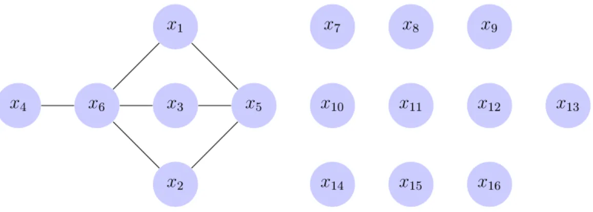
x4 x6 x1 x3 x2 x5 x7 x8 x9 x10 x11 x12 x13 x14 x15 x16
Figure 6: The graph for (26) produced according to the techniques setout in Section 5. Despite being a larger system the minimum vertex cover{x5, x6} is still small. All other
variables form a maximum independent set, which can be eliminated with linear methods.
26. The connection graph is given in Figure 6 showing that {x5, x6} as a minimum vertex cover. We obtain the simplified system:
3796549898085k29x35x6+ 71063292573000k29x35 +106615407090630k29x25x26+ 479383905861000k29x25x6 +299076127852260k29x5x36+ 3505609439955600k29x5x26 +91244417457024k29x46+ 3557586742819200k29x36 −598701732300k30x35x6− 83232870778950k30x25x 2 6 −185019487578700k30x5x36− 3796549898085x 4 5x6 −71063292573000x4 5− 106615407090630x 3 5x 2 6 − 479383905861000x3 5x6− 299076127852260x 2 5x 3 6 −3505609439955600x2 5x 2 6− 91244417457024x5x 4 6 −3557586742819200x5x36 = 0, 3796549898085k28x35x6+ 71063292573000k28x35 +106615407090630k28x25x 2 6+ 479383905861000k28x25x6 +299076127852260k28x5x36+ 3505609439955600k28x5x26 +91244417457024k28x46+ 3557586742819200k28x36 −3197848165785k30x35x6− 23382536311680k30x25x26 −114056640273560k30x5x36− 91244417457024k30x46 −3796549898085x3 5x 2 6− 71063292573000x 3 5x6
− 106615407090630x2 5x 3 6− 479383905861000x 2 5x 2 6 −299076127852260x5x46− 3505609439955600x5 x36 − 91244417457024x56− 3557586742819200x46 = 0.
along with positivity constraints x6 > 0, x5 > 0, k30 > 0, k29 > 0, and k28 > 0.
9. Grid Sampling: Symbolic vs Numeric
In this section we summarise work that was first presented in CASC 2017 (England et al., 2017) which compared the use of symbolic and numeric techniques to identify multistationary regions via grid sampling.
9.1. Algorithms and Software
In this section we will use Symbolic Grid Sampling: so we have results only for a set of numerical sample points, but each sample point will undergo a symbolic computation. The result will still be an approximate identifica-tion of the region, since the sampling will be finite, but the results at those sample points will be guaranteed free of numerical errors. The symbolic computations follow exactly the strategy introduced in Section 4 except each sample point will set all parameters (rather than leaving one free) meaning a simpler symbolic computation than in Section 4 performed multiple times. In particular, with no free parameters the Lazy variant of Real Triangular-ization (LRT) used in Section 4 gives the full solution (no laziness) as we would get from Real Triangularization (RT) and so we just use the latter.
We will compare this symbolic grid sampling with a fully numerical gird sampling approach using the homotopy solver Bertini developed by Bates et al. (2013), in its standard configuration to compute complex roots. Alter-natives to Bertini include PHCpack by Verschelde (2011) and the Numerical Algebraic Geometry package for Macaulay2 by Leykin (2011). Reasons for choosing Bertini include that it is the most cited homotopy solver for the past 8 years and that it allows adaptive and very high-precision arithmetic (whereas PHCpack only allows double-double)9. We parsed the output of
9We note that a recent development for Bertini published after this article was in
press could be applicable to this problem: Paramotopy by Bates et al. (2018) allows for parallelism and computation reuse, well suited for such grid sampling.
Bertini using Python, and determined numerically which of the complex roots are real and positive using a threshold of 10−6 for positivity.
Bertini computations (v1.5.1) were carried out on a Linux 64 bit Desk-top PC with Intel i7. Maple computations (v2016 with April 2017 Regular Chains) were carried out on a Windows 7 64 bit Desktop PC with Intel i5.
Software Remark 2. For the reduced system of Model 28 Bertini (incor-rectly) could not find any roots, not even complex ones, for any of the pa-rameter settings. The situation did not change when going from adaptive precision to a very high fixed precision. However, we have not attempted more sophisticated techniques like providing user homotopies. It seems a bug in Bertini has been triggered by this problem instance. It has been reported to the developers.
9.2. Sample Ranges and Plots
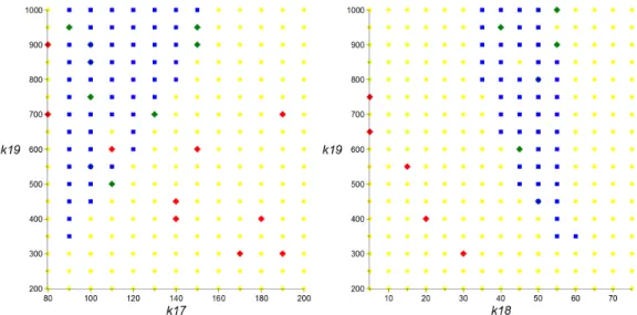
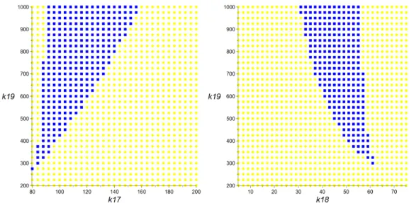
For Model 26 we will use a sampling range for k19 from 200 to 1000 by 50; for k17 from 80 to 200 by 10; and for k18 from 5 to 75 by 5.
For Model 28 we will use a sampling range for k30 from 100 to 1600 by 100; for k28 from 40 to 160 by 10; and for k29 from 120 to 240 by 10.
We produce 2d plots in each case with the third parameter fixed to its values indicated in (4) and (29). In those plots we will colour sample points according to the number of fixed points observed: yellow discs indicate one fixed point and blue boxes three. Diamonds indicate numerical errors where zero (red) or two (green) fixed states were identified.
9.3. Results and Comparison
The plots produced by the grid sampling are presented in Figures 7−10; and the time taken to produce them is summarised in Table 2.
9.3.1. Comparison of models
Model 28 forms a larger real algebraic problem than Model 26, 16 vari-ables and equations rather than 11, so it unsurprising that it takes longer to perform computations.
Regarding the symbolic computations: Model 28 requires an actual CAD of a plane to be produced for each sample point while Model 26 only real root isolation (decomposition of a line). This was the case regardless of whether the original or reduced system was used as the starting point, since the RT preprocessing also reduced the number of variables that needed analysis by
CAD. We note that even with the reduced system it was still beneficial to pre-process CAD with RT: the average time per sample point with pre-pre-processing (and including time taken to pre-process) was 0.485 seconds while without it was 3.577 seconds. It is not clear if this is because of a genuine simplification or because the CAD algorithm from the Regular Chains Library that we used it particularly tuned for triangular systems.
9.3.2. Effects of the pre-processing in Section 5
Figure 7 and Figure 8 both refer to Model 26. The latter is produced by Maple’s symbolic calculations and so guaranteed free of numerical error. The former, Figure 7, represents the output of Bertini on the original system. We see that there are numerous numerical errors present: the rouge red and green diamonds in Figure 7. We find that when computing with the reduced system rather than the original system Bertini was able to to avoid all these errors, producing the same plots as Maple in Figure 8.
With Model 28 we see similar numerical errors from Bertini in Figure 9 when compared with Maple in Figure 10. However, in the case of Model 28 the reduction led to catastrophic effects for Bertini: built-in heuristics quickly (and incorrectly) concluded that there are no zero dimensional solu-tions for the system, and when switching to a positive dimensional run also no solutions could be found.
From the timing data in Table 2 we see that both Bertini and Maple benefited from the reduced system: For Model 26 Bertini took a third of the original time while Maple took a tenth of the original. For Model 28 the speed-up enjoyed by the symbolic method from the pre-processing was even greater: almost 100 fold!
Table 2: Timing data (in seconds) of the grid samplings described in Section 9. Numerical is using Bertini and Symbolic the Regular Chains Library for Maple.
Numerical Symbolic
Model Mean Mean Median StdDev Maximum 26 – Original 2.4 0.568 0.530 0.107 0.905 26 – Reduced 0.85 0.053 0.047 0.036 0.343 28 – Original 16.57 42.430 40.529 8.632 84.116 28 – Reduced ⊥ 0.485 0.468 0.119 0.796