HAL Id: hal-01102049
https://hal.inria.fr/hal-01102049
Submitted on 12 Jan 2015HAL is a multi-disciplinary open access
archive for the deposit and dissemination of sci-entific research documents, whether they are pub-lished or not. The documents may come from teaching and research institutions in France or abroad, or from public or private research centers.
L’archive ouverte pluridisciplinaire HAL, est destinée au dépôt et à la diffusion de documents scientifiques de niveau recherche, publiés ou non, émanant des établissements d’enseignement et de recherche français ou étrangers, des laboratoires publics ou privés.
Multi-Rate Mass Transfer (MRMT) models for general
diffusive porosity structures
Tristan Babey, Jean-Raynald de Dreuzy, Céline Casenave
To cite this version:
Tristan Babey, Jean-Raynald de Dreuzy, Céline Casenave. Multi-Rate Mass Transfer (MRMT) models for general diffusive porosity structures. Advances in Water Resources, Elsevier, 2015, 76, pp.146-156. �10.1016/j.advwatres.2014.12.006�. �hal-01102049�
Multi-Rate Mass Transfer (MRMT) models for general
1
diffusive porosity structures
2
Tristan Babey1, Jean-Raynald de Dreuzy1, Céline Casenave2,3 3
1
Géosciences Rennes (UMR CNRS 6118), Campus de Beaulieu, Université de Rennes 1, 4
35042 Rennes cedex, France 5
2
UMR INRA-SupAgro 0729 MISTEA, 2 place Viala 34060 Montpellier, France 6
3
MODEMIC project-team, INRA/INRIA, Sophia-Antipolis, France 7
Corresponding author: Tristan Babey, +33646204318, [email protected] 8
Highlights: 9
A mobile-immobile transport model with a structured immobile domain is proposed
10
Structured INteracting SINC generalize Multiple INteracting
Continua-11
MINC 12
Whatever the SINC structure, a unique equivalent MRMT model exists
13
MRMT models with only very few rates accurately model conservative transport
14
We propose a robust numerical identification of the first few rates 15
ABSTRACT
16
We determine the relevance of Multi-Rate Mass Tansfer (MRMT) models to general diffusive 17
porosity structures. To this end, we introduce Structured INteracting Continua models (SINC) 18
as the combination of a finite number of diffusion-dominated interconnected immobile zones 19
exchanging with an advection-dominated mobile domain. It directly extends Multiple 20
INteracting Continua framework [Pruess and Narasimhan, 1985] by introducing a structure in 21
the immobile domain, coming for example from the dead-ends of fracture clusters or poorly-22
connected dissolution patterns. We demonstrate that, whatever their structure, SINC models 23
can be made equivalent in terms of concentration in the mobile zone to a unique Multi-Rate 24
Mass Transfer (MRMT) model [Haggerty and Gorelick, 1995]. We develop effective shape-25
free numerical methods to identify its few dominant rates, that comply with any distribution 26
of rates and porosities. We show that differences in terms of macrodispersion are not larger 27
than 50% for approximate MRMT models with only one rate (double porosity models), and 28
drop down to less than 0.1% for five rates MRMT models. Low-dimensional MRMT models 29
BABEY ET AL.: MRMT MODELS FOR GENERAL DIFFUSIVE POROSITY STRUCTURES
2 accurately approach transport in structured diffusive porosities at intermediate and long times 30
and only miss early responses. 31
32
Keywords: Porous media; Solute transport; Mobile-immobile models; Multi-Rate Mass 33
Transfer; 34
BABEY ET AL.: MRMT MODELS FOR GENERAL DIFFUSIVE POROSITY STRUCTURES
3
1 Introduction
35
Transport in complex geological environments results in part from the interactions between 36
fast advective-dominated transport in a localized "mobile porosity" and slow diffusive-37
dominated transport in extensive "immobile porosities". It is the case of the fracture-matrix 38
systems [Neretnieks, 1980; Tang et al., 1981] and of the highly heterogeneous porous media 39
[Fernandez-Garcia et al., 2009; Golfier et al., 2007; Gotovac et al., 2009; Willmann et al., 40
2008]. When diffusive times in the immobile zones become much larger than the 41
characteristic advective time in the mobile zone, transport becomes anomalous with non-42
Gaussian concentration plumes, more extensive spreading and mixing, slow transit times, and 43
broad ranges of solute retardation times [Berkowitz et al., 2006; Dentz et al., 2004]. Such 44
transport mechanisms and exchanges are at the root of numerous anomalous transport 45
modeling frameworks [Benson and Meerschaert, 2009; Benson et al., 2000; Berkowitz and 46
Scher, 1998; Carrera et al., 1998; Cushman and Ginn, 2000; Haggerty and Gorelick, 1995]
47
and can be highly effective in the interpretative and predictive phases of laboratory and field 48
experiments [Benson et al., 2001; Berkowitz et al., 2000; Gouze et al., 2008; Haggerty et al., 49
2001; Haggerty et al., 2004]. Anomalous transport ultimately stems from some extended 50
distribution whether it is a waiting time distribution as in Continuous Time Random Walk 51
(CTRW) or a rate-porosity distribution as in Mutli-Rate Mass Transfert (MRMT) [Dentz and 52
Berkowitz, 2003; Neuman and Tartakovsky, 2009; Silva et al., 2009]. For MRMT models,
53
while these distributions can take very different shapes [Haggerty et al., 2000], only some 54
power-law distributions are effectively related to diffusive processes in 1D, 2D or 3D 55
inclusions [Carrera et al., 1998; Haggerty and Gorelick, 1995] or to anomalous diffusive 56
processes in fractal-like structures [Haggerty, 2001]. Diffusive structures may however be 57
topologically more complex like for example for fracture dead ends [Flekkøy et al., 2002; 58
Sornette et al., 1993], fracture-matrix interactions [Jardine et al., 1999; Karimi-Fard et al.,
59
2006; Sudicky and Frind, 1982; Tang et al., 1981; Tsang, 1995], or dissolution patterns in 60
porous media [Golfier et al., 2002; Luquot et al., 2014] (Figure 1). 61
In this article, we show that the MRMT framework is general to all diffusive architectures that 62
can be modeled as a finite number of interconnected continua (Figure 1). The notion of 63
continuum comes from the double porosity and Multiple INteracting Continua (MINC) 64
concepts introduced initially for fracture-matrix systems [Pruess and Narasimhan, 1985; 65
Warren et al., 1963]. The double porosity model is the classical diffusive interaction of
66
advective-diffusive processes in a mobile zone with a single immobile zone like in double-67
BABEY ET AL.: MRMT MODELS FOR GENERAL DIFFUSIVE POROSITY STRUCTURES
4 porosity models [Warren et al., 1963]. The Multiple INteracting Continua (MINC) framework 68
models matrix diffusion as diffusive-like exchanges within a succession of "continua", 69
identified to the elementary cells issued by a finite-difference discretization of the diffusion 70
process in the matrix (Figure 2a) [Pruess, 1992; Pruess and Narasimhan, 1985]. The 71
denomination of multiple continua is a direct generalization of the double porosity concept of 72
Warren and Root [1963]. We propose to further generalize the notion of interacting continua
73
to any immobile zones structure where diffusive-like exchanges intervene between any 74
connected zones or continua. Because of the potential importance of structure on diffusion, 75
we denote these models as Structured INteracting Continua (SINC). SINC models include a 76
wide range of structures going from elementary branching and loops (Figure 2b and c) to 77
more involved dissolution patterns (Figure 2d). They would typically be derived from the 78
coarse discretization of diffusion processes in dead-end porosity structures [Gouze et al., 79
2008; Noetinger and Estebenet, 2000]. We define SINC models in section 2, with their exact 80
relation to the MRMT and MINC models. We show in section 3 that any SINC model is 81
equivalent in terms of transport to a unique MRMT model of the same dimension, i.e. with the 82
same number of immobile zones. We develop efficient numerical methods in section 4 to 83
identify lower-dimension but highly accurate approximate MRMT models. 84
(a) Limestone dissolution structure [Luquot et al., 2014] (b) SINC model (c) Equivalent MRMT model
Figure 1: (a) Skeleton of a dissolution feature in an oolitic limestone, observed by X-ray micro-tomography [Luquot et al., 2014]. The dissolving 85
acidic solution percolates from top to bottom on the general view (bottom left). Its pH increases from top to bottom and from inside out of the 86
main flow path indicated by the curved arrow on the detailed view (top right). The acid dissolves preferentially the calcite cement surrounding 87
the oolites, the size of the pores progressively decreases away from the main flow path, and the organization of the pores becomes more complex. 88
(b) Structured INteracting Continua model (SINC) sketched from the dissolution pattern of (a) with three cross sections transversal to the mobile 89
zone materialized by the arrow. (c) Equivalent MRMT model with the 5 most important rates as determined by the numerical methods set up in 90
section 4. The size of the boxes scales with the porosity affected to the rates labeled by triangles in Figure 7. 91
(a) MINC 1D (b) Asymmetric Y (c) Asymmetric loop (d) Dissolution pattern
Figure 2: Examples of Structured INteracting Continua (SINC) used to illustrate and validate the numerical identification methods of the 93
equivalent MRMT models. From left to right, the diffusive porosity structures are (a) the classical Multiple INteracting Continua (MINC) 94
[Pruess and Narasimhan, 1985], (b) an asymmetric Y with a single junction, (c) an asymmetric loop, and (d) the dissolution structure presented 95
in Figure 1. The size of the immobile cells is proportional to their porosity and the distance along the immobile structure is to scale. The mobile 96
zone is represented by the thick black box with the crossing arrow. Its size has been exaggerated 10 times to be clearly marked. To be 97
comparable, the four structures have the same total porous volume and the same radius of gyration taken with respect to the mobile zone. 98
2 Structured INteracting Continua (SINC)
100
We present the Structured INteracting Continua framework (SINC) and show how it relates to 101
existing models like Multi-Rate Mass Transfer (MRMT) and Multiple INteracting Continua 102
(MINC). 103
The SINC model is made up of a continuous 1-D mobile zone in interaction with a finite 104
number of interconnected immobile zones (Figure 1). In the continuous mobile zone, solutes 105
are transported by advection, dispersion and diffusion. Between the mobile zone and the 106
immobile zones as well as between the immobile zones, concentration exchanges are 107
diffusive-like, i.e. directly proportional to the difference of concentrations. This model can be 108
generically expressed as: 109
R U
L AU t U m (1)where U [cm(x,t) c1im(x,t) cimN(x,t)]T is the vector of dimension N+1 made up of the 110
concentrations in the mobile zone cm
x,t and in the N immobile zones c
x ti
im , with
111
N
i1,..., . A is the (N 1,N 1) interaction matrix characterizing the diffusive-like 112
concentration exchanges between the immobile zones and with the mobile zone. Rm is the
113
restriction matrix to the mobile zone: 114
i, j
i1 j1
Rm . (2)
L is the transport operator in the mobile zone:
115
2 2 x c d x c q c L m m m m m (3)with q, m and dm the Darcy flow, porosity and dispersion coefficient in the mobile zone. 116
The physical properties of the mobile and immobile domains are homogeneous along the 117
mobile domain. The interaction matrix A is equal to the matrix M deriving from the diffusive-118
like mass exchanges between the different zones, corrected by their porosities: 119
M
BABEY ET AL.: MRMT MODELS FOR GENERAL DIFFUSIVE POROSITY STRUCTURES
8 with the diagonal matrix whose diagonal elements are the porosities associated to the 120
mobile zone m and to the N immobile zones imi with i1,...,N : 121
1 , 1 , for , , 1 , 1 1 j i j i j i imi m . (5)The matrix M expresses rates of mass exchange. The dimension of its elements is therefore 122
the inverse of a time. As exchanges are diffusive-like, M is a M-matrix, i.e. M is symmetric, 123
its diagonal elements are positive, its off-diagonal elements are negative or equal to zero, and 124
the sum of its elements along each of its rows is equal to zero. We underline that it is the 125
matrix M that is symmetric and generally not the interaction matrix A that also integrates the 126
differences in porosities. The interaction matrix A registers the connectivity of the different 127
zones through the position of its non-zero off-diagonal elements, the strength of the 128
interactions is determined by porosity ratios and exchange rates. Figure 3a shows the example 129
of the interaction matrix for the asymmetric Y structure (cf Figure 2b). The branching 130
architecture leads to a compact interaction matrix, which values are all on the three principal 131
diagonals except at the branching node. The interaction matrix is scaled by the inverse of the 132
mean diffusion time in the immobile structure . We define as the quadratic mean distance 133
of the immobile zones to the mobile zone divided by the diffusion coefficient between two 134
zones. 135
The SINC framework generalizes Multiple INteracting Continua (MINC) [Pruess and 136
Narasimhan, 1985]. MINC models are obtained by the finite-difference discretization of
137
diffusion in a 1-D homogeneous medium. In such a case, the interaction matrix A is simply 138
tri-diagonal. The term "continuum" comes from the continuity along the mobile zone like in 139
the dual-porosity concept [Warren et al., 1963]. It is consistent with our concept of a 140
continuous formalism of transport along the mobile zone and a finite number of interacting 141
continua in the immobile direction. 142
The SINC framework also generalizes Multiple-Rate Mass Transfer models with a finite 143
number of rates [Carrera et al., 1998; Haggerty and Gorelick, 1995]. In MRMT models as 144
defined by Haggerty et al. [1995], the immobile domain consists in a distribution of sub-145
domains exchanging exclusively with the mobile domain. The star-like connectivity structure 146
leads to an arrow-type broad-width interaction matrix (Figure 3b). Each sub-domain is 147
characterized by its rate of transfer i and its porosity i im
, with i i1[Haggerty and
BABEY ET AL.: MRMT MODELS FOR GENERAL DIFFUSIVE POROSITY STRUCTURES
9
Gorelick, 1995]. When defined with a finite number of rates, MRMT models can be recovered
149 by fixing 150
) 1 , 1 ( ) , ( for , , 1 , 1 , , 1 for , 1 1 , and 1 , 1 for 0 , 1 , 1 1 j i j i j i j i M i i M i i M i M j i j i j i M i im m i j j i i im . (6)Because they are defined in algebraic terms, SINC models can only represent MRMT models 151
with finite number of rates. They are rigorously not equivalent to 1D, 2D and 3D diffusion 152
models that themselves correspond to an infinite number of exchange rates [Haggerty and 153
Gorelick, 1995]. However they offer very accurate approximations when taking only a finite
154
number of rates, especially as the porosities i im
decrease as a power law of i. SINC models
155
generalize MRMT models defined with a finite number of rates but remain different to 156
MRMT models defined by an infinite serie of rates or by a continuous rate-porosity function. 157
Our objective in this article is not to produce any kind of generalization of MRMT models but 158
rather to determine how complex diffusive porosity structures can be approached by simpler 159
reduced models. 160
(a)
(b)
Figure 3: Diffusive porosity structures represented as cross-sections transversal to the mobile 161
zone direction ((a),(b)), with their associated interaction matrix A ((c),(d)) for the asymmetric 162
Y (top) and MRMT structures (bottom). Dotted frames around subsets of the immobile 163
porosity structures ((a) and (b)) and around matrix lines ((c) and (d)) show how structures are 164
translated in matrix form. Parameters for the asymmetric Y structure are taken from Table 1 165
and the multiplicative factor (=5.015) is equal to the ratio of the distance between two 166
consecutive immobile zones to the radius of gyration of the immobile domain to the mobile 167
zone. is the ratio of the total immobile porosity to the mobile porosity. 168
(c)
3 Proof of equivalence of SINC to MRMT model
169
Following up the work of Haggerty and Gorelick [1995], we define the equivalence relation 170
to a MRMT model as the identity of the mobile concentration at any time. To prove the 171
equivalence of the SINC model to a MRMT model, we first decompose the interaction matrix 172
A in two parts, consisting in the exchanges between the immobile zones only for the first part
173
and in the exchanges between the mobile zone and the immobile zones for the second one: 174 1 , 1 21 1 , 1 12 11 0 0 0 0 N N A A A A A A A (7)
with A A(2N 1,2N 1). As shown in Appendix A, the matrix A can be diagonalized 175 1 R R A (8)
with the diagonal matrix made up of the eigenvalues of A, which are all real and negative, 176
and R the matrix of the eigenvectors of A, defined each up to a multiplicative constant. To 177
fix the eigenvalues decomposition, as is defined up to a permutation of its diagonal 178
elements, we sort the eigenvalues according to their absolute value by increasing order 179
1 , 1 ,
ii i i . In the new coordinate system defined by the eigenvectors, there are no more
180
exchanges between the immobile zones. All exchanges are made directly between the 181
immobile zones and the mobile zone. To characterize the precise nature and extent of these 182
exchanges, we propagate the change of the coordinate system to the exchanges with the 183 mobile zone 184 1 1 , 1 21 1 , 1 12 11 1 , 1 21 1 , 1 12 11 0 0 R B B B B A R A A A A A N N N N (9)
with the (N 1,N 1) matrix R and its inverse 1
R defined as
BABEY ET AL.: MRMT MODELS FOR GENERAL DIFFUSIVE POROSITY STRUCTURES 12 0 0 0 0 1 R R and 0 0 0 0 1 1 1 R R . (10)
In this transformation, the mobile zone remains unchanged consistently with our objective to 186
reorganize only the immobile zones without interfering with the concentration in the mobile 187
zone. The full transformation defined by R is applied to the matrix A following its 188 decomposition in equation (7) 189 1 1 , 1 21 1 , 1 12 11 1 0 0 0 0 R B B B B A R R R A N N (11)
which can be finally expressed by a simple factorization as 190 1 RBR A with 1 , 1 21 1 , 1 12 11 N N B B B B A B . (12)
Finally, as the restriction matrix to the mobile zoneRm (equation (2)) commutes with R1, we
191
can write the full model as 192
R R U
L U BR t U R m 1 1 1 . (13)To be representative of a MRMT model, B should be an arrow matrix, the sum of its elements 193
over each of its rows should be zero, and all its non-diagonal elements must be either positive 194
or equal to zero. In Appendix B, we show that this can be obtained by adjusting the norm of 195
the eigenvectors in R. The characteristics of this MRMT model are then determined by a 196
simple identification of equation (6) with equation (12): 197
BABEY ET AL.: MRMT MODELS FOR GENERAL DIFFUSIVE POROSITY STRUCTURES 13 i i m i i m i im i i B B B 1, 1 1 , 1 1 , 1 . (14)
While this algebraic identification method can already be widely used to determine equivalent 198
MRMT models, it faces some numerical limitations. The diagonalization process becomes 199
challenging when Aˆ becomes large, limiting the range of the identification to not too 200
complex architectures and/or coarse discretizations of the immobile domain. The immobile 201
porosity structure may be composed of a large number of cells, while a much smaller number 202
of rates may be necessary to get highly accurate equivalent MRMT models. To address these 203
limitations, we propose an alternative approximate numerical identification method. 204
4 Approximate numerical identification method of the MRMT model equivalent to a
205
SINC model
206
We first develop the numerical methodology and secondly apply it to the four examples of 207
Figure 2. Because of their widely differing structures, these four SINC examples are thought 208
to be a good basis for testing and illustrating the numerical methods. The first one is the 209
classical MINC taken as reference. The two next ones were chosen for their elementary 210
branching and looping connectivity patterns (Figure 2b and c). Any more involved patterns 211
like the dissolution pattern of Figure 2d will be some kind of combination of these elementary 212
structures. These four examples are comparable in the sense that they have the same mobile 213
properties, the same overall immobile to mobile porosity ratio , and the same mean quadratic 214
diffusion time as defined in section 2 (Table 1). The dispersivity in the mobile zone 215
m
m q
d / / divided by the effective dispersivity due to the exchanges with the immobile zone
216
defined as
q/m
is taken equal to 5.105, i.e. much smaller than 1, so that dispersive effects 217come predominantly from the mobile/immobile exchanges. For the same reason, is taken 218
much larger than 1 ( 100). 219
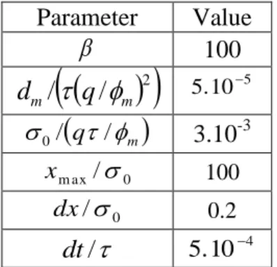
Parameter Value 100
2
/ / m m q d
5.105
q m
0/ / 3.10-3 0 m ax/ x 100 0 / dx 0.2 / dt 5.104Table 1: Parameters used for the simulation of section 4.2 with the characteristic diffusion 220
time and the consecutive distance covered by advection in the mobile zone q/m as 221
temporal and spatial dimensional parameters. is the immobile to mobile porosity ratio. 222
2
/ / m m qd
is the dimensionless dispersion in the mobile zone. 0/
q /m
is the223
dimensionless standard deviation of the initial Gaussian concentration profile. xm axis the
224
extension of the simulation domain in the direction of the mobile zone, dx is the spatial step 225
along the mobile zone and dt is the time step. 226
4.1 Methodology
227
To numerically approximate the MRMT model equivalent to a SINC model, we consider the 228
particular case of the discharge of the immobile zones to the mobile zone. The mass 229
discharged to the mobile zone from an initially homogeneous immobile concentrations c0 is
230
fitted by a combination of exponential functions typical of the MRMT model. The residual 231
mass per unitary volume m(t) in the immobile domains is fitted by its MRMT counterpart 232 ) (t given by: 233
N i i i im t c t 1 0 exp( ) ) ( (15) where i and i im , i1N are the N rates and immobile porosities defined in equation (6). 234
In Appendix C, we develop an optimization method to identify the and im series. We 235
further illustrate its application to the cases N 1 and N 2 in Appendix D. 236
The advantage of this method over the previous algebraic method is to be flexible in terms of 237
the number of rates N to identify. It also prioritizes the identification of the rates and 238
immobile porosities having a significant impact on transport. In the following we determine 239
the number of rates that should be identified to model accurately macrodispersive processes. 240
4.2 Simulations and results
241
We analyze the influence of the number of rates N on the reproduction of macrodispersion for 242
the four structures displayed in Figure 2 for N ranging from 1 to 5. Identification is performed 243
according to the methodology presented before and with a logarithmic sampling of times 244
starting at the time for which the relative mass discharge to the mobile zone is lower than 10-3 245
and ending at the time for which the relative residual mass itself is lower than 10-4. 246
Simulations of transport for the SINC and approximate MRMT models are further performed 247
with identical Gaussian concentration profiles in the mobile and immobile domains 248 2 0 2 0 0 max 2 ) ( exp 2 ) 0 , ( ) 0 , ( x x c t x c t x cm im (16)
where x0, 0 and cm ax are the mean, standard deviation and maximum concentration of the
249
Gaussian profile. 0 is taken small enough so that the initial plume size has minor effects on
250
the overall dispersion (Table 1). 251
BABEY ET AL.: MRMT MODELS FOR GENERAL DIFFUSIVE POROSITY STRUCTURES
16 We compute for all models the effective dispersion coefficient D as
252 dt d D x 2 2 1 (17)
with x the plume spreading 253 2 0 1 0 2 2 ) / ( /m m m m x . (18)
The spatial moments of concentration mk are given by 254
0 1 1 ) , , ( ) , ( ) ( x N i k k t x i i U x t i dx m . (19)We assess the quality of the MRMT model for modeling dispersion through the quadratic 255
mean of the relative difference in effective dispersion of the SINC and MRMT models: 256
t t SINC MRMT MRMT SINC MRMT SINC dt dt t D t D t D t D D D diff 2 2 / )) ( ) ( ( ) ( ) ( ) , ( . (20)This criterion is sensitive to differences in dispersion on a broad time range from the initial 257
time to the time at which dispersion becomes constant. 258
Classical numerical methods were used to solve both the exchanges within the immobile 259
zones and the advective-dispersive transport in the mobile zone [de Dreuzy et al., 2013]. They 260
were validated on a set of immobile structures rigorously equivalent to the MINC model 261
(Figure 4). In those cases, diff(DSINC,DMINC) was of the order of 10
-11
and much smaller than 262
any differences recorded in the analysis performed hereafter. 263
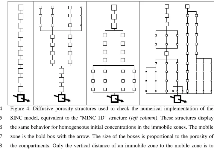
Figure 4: Diffusive porosity structures used to check the numerical implementation of the 264
SINC model, equivalent to the "MINC 1D" structure (left column). These structures display 265
the same behavior for homogeneous initial concentrations in the immobile zones. The mobile 266
zone is the bold box with the arrow. The size of the boxes is proportional to the porosity of 267
the compartments. Only the vertical distance of an immobile zone to the mobile zone is to 268
scale. 269
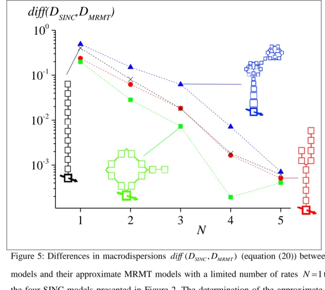
For the structures displayed on Figure 2, the effective dispersion obtained with the MRMT 270
models converges quickly to the reference dispersion of the corresponding SINC model 271
(Figure 5). The equivalent MRMT model with only one immobile zone (N=1), equivalent to 272
the double porosity model [Warren et al., 1963], already gives the right order of magnitude of 273
dispersion. With N=2, the error of the MRMT model is close to10%. With N=4, it is close to 274
1% and with N=5, it is close to 0.1%. A very limited number of rates is thus sufficient to 275
represent even the complex diffusive structure displayed by Figure 2d. This fundamentally 276
comes from the homogenization nature of diffusion that systematically removes the extremes 277
of the concentration distributions as previously noted in numerous studies [Haggerty and 278
Gorelick, 1995; Villermaux, 1987].
279
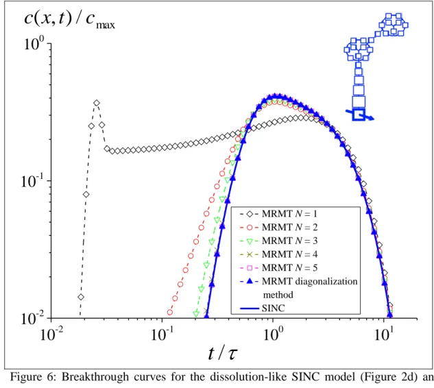
In addition, the equivalent MRMT model with only one rate reproduces well the tailing of the 280
breakthrough curve (Figure 6). As expected, introducing higher rates progressively improves 281
the accuracy of the MRMT model at earlier times. The double peak observed for N=1 is a 282
classical feature of double porosity models where advection is much faster than diffusion in 283
the immobile porosity [Michalak and Kitanidis, 2000]. It vanishes for higher-order MRMT 284
models (N=2 to 5), as higher rates enhance short-term mobile-immobile exchanges and 285
remove early breakthroughs. 286
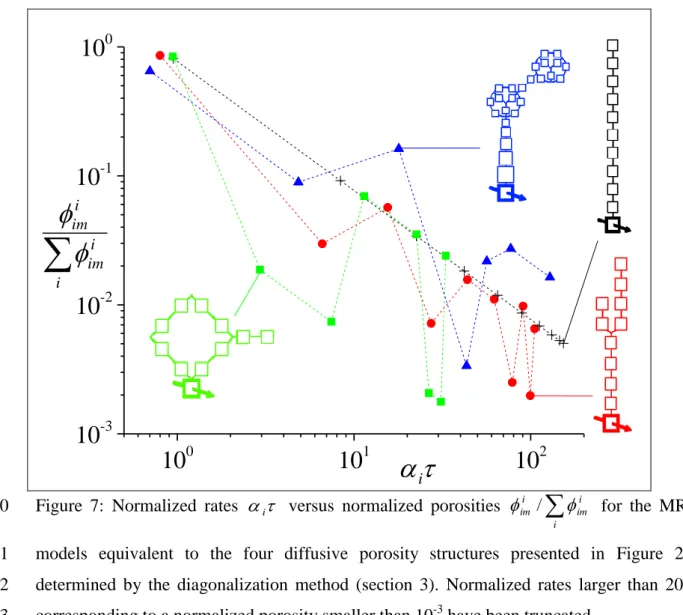
The quality of the MRMT model with only very few rates fundamentally comes from the 287
dominating role of the smaller rates (i.e. larger transfer times). In fact the whole rate series as 288
determined by the algebraic diagonalization method shows that the lowest rate dominates in 289
every case by accounting for 70% to 85% of the total immobile porosity (Figure 7). The five 290
lowest rates represent at least 95% of the total immobile porosity for all the studied structures. 291
The evolution of the porosities i im
with the rates i is monotonic only for the MINC model
292
and becomes much more variable for more complex structures, highlighting the need of 293
identification methods that do not assume any a priori repartition of the immobile porosity 294
among the rates. We finally note that our results pertain to complex diffusive structures 295
observed on a given range of scales. If not close to the mobile zone, finer details would be fast 296
homogenized by diffusion and are unlikely to modify the identified rates. If close to the 297
mobile zone, finer details should be treated independently in the same way as for the larger-298
scale structures and the MRMT models obtained at different scales should be eventually 299
superposed. 300
1
2
3
4
5
10
-310
-210
-110
0diff(D
SINC,D
MRMT)
N
Figure 5: Differences in macrodispersions diff(DSINC,DMRMT) (equation (20)) between SINC 301
models and their approximate MRMT models with a limited number of rates N1 to5, for 302
the four SINC models presented in Figure 2. The determination of the approximate MRMT 303
models is achieved with the numerical identification method in the temporal domain (Section 304
4.1 and Appendix C). 305
MRMT N = 1 MRMT N = 2 MRMT N = 3 MRMT N = 4 MRMT N = 5 MRMT diagonalization method SINC
10
-210
-110
010
110
-210
-110
0 max/
)
,
(
x
t
c
c
/
t
Figure 6: Breakthrough curves for the dissolution-like SINC model (Figure 2d) and for its 306
equivalent MRMT models, either determined by the diagonalization method (section 3), or by 307
the numerical method in the temporal domain with a limited number of N rates (Section 4.1 308
and Appendix C). The concentrations are measured at the position x200.
10
010
110
210
-310
-210
-110
0
i i im i im
iFigure 7: Normalized rates i versus normalized porosities
i i im i im / for the MRMT 310
models equivalent to the four diffusive porosity structures presented in Figure 2, as 311
determined by the diagonalization method (section 3). Normalized rates larger than 200 or 312
corresponding to a normalized porosity smaller than 10-3 have been truncated. . 313
5 Conclusion
314
We define a general mobile/immobile Structured INteracting Continua (SINC) transport 315
framework accounting for a broad variety of immobile porosity structures. Like in more 316
classical double porosity, Multi-Rate Mass Transfer (MRMT), and Multiple INteracting 317
Continua (MINC) frameworks, solute transport is dominated by advection in the mobile 318
porosity and is diffusion-like in the immobile porosity. The SINC framework introduces a 319
connectivity pattern within the immobile zone covering a broad range of diffusive geological 320
structures including cluster of dead-end fractures, irregular matrix shapes and dissolution 321
patterns. Immobile structures are based on branching and looping structures, and on any 322
combination of them. Solute transport is expressed as an advection-diffusion equation coupled 323
to algebraically defined exchanges with a finite number of immobile zones. Interactions 324
among the immobile zones and with the mobile zone are fully determined by a simple 325
interaction matrix, which resumes to an arrow type of matrix in the MRMT case and to a tri-326
diagonal matrix in the MINC case. The graph of the matrix registers the connectivity pattern 327
while the value of its coefficients comes from relative porosities and strength of exchanges 328
between immobile zones. 329
We show that any Structured INteracting Continua model is equivalent to a unique MRMT 330
model, where the equivalence is defined as the strict identity of the concentrations in the 331
mobile zone, whatever the initial and boundary conditions. The rates of the equivalent MRMT 332
model are the eigenvalues of the subset of the interaction matrix where the line and column 333
corresponding to the mobile zone are removed. The diagonalization method gives a first 334
identification method of the equivalent MRMT with the same dimension, i.e. with the same 335
number of immobile zones. Because of limitations coming essentially from the dimension of 336
the immobile porosity structure, we set up alternative numerical methods designed to identify 337
the most important rates controlling the transport of solute. Developed both in the temporal 338
and Laplace domains, these methods seek for the combination of a finite number of 339
exponential functions that best matches a simple discharge of the immobile zones within a 340
quickly flushing mobile zone. 341
A simple sensitivity study on representative diffusive structures shows that very few rates are 342
needed for accurately modeling the solute transport in a 1D advection-dominated mobile zone 343
exchanging with an immobile porosity structure. Double porosity models (MRMT with a 344
single rate) already give the right order of magnitude of macrodispersion. Differences in 345
BABEY ET AL.: MRMT MODELS FOR GENERAL DIFFUSIVE POROSITY STRUCTURES
23 macrodispersion drop down to around 10% for two rates, to 1% for four rates, and to less than 346
0.1% for five rates. Simplified models based on only five rates approach accurately the 347
behavior of the system at intermediate to large times and only miss the very early responses. 348
While only few rates are necessary, their distribution and associated porosities are highly 349
variable, the complexity of the structure being transferred to the identified rates and 350
associated porosities. We thus conclude that MRMT models can be very efficient for 351
modeling diffusion-like transport in a broad range of porosity structures with only very few 352
rates. Even though numerical simulations have been done in 1D mobile domains, results are 353
likely generalize to 3D. Additional simulations should also be performed to investigate the 354
behavior of mixing and chemical reactivity both between different SINC structures and 355
between the SINC structures and their simplified MRMT counterparts. 356
BABEY ET AL.: MRMT MODELS FOR GENERAL DIFFUSIVE POROSITY STRUCTURES
24
Appendix A: Diagonalization of A
357
We show that the eigenvalues of the matrix A are real and negative and that they correspond 358
to the opposites of the rates of the equivalent MRMT model (i). As displayed by 359
equations (4) and (7), A1M where
) 1 2 , 1 2 ( N N and 360 ) 1 2 , 1 2 ( M N N
M . 1 is diagonal and its diagonal elements are all positive.
361
Thus 1 is positive definite, i.e. for every non-zero and real column vector x, 362 0 ) , ( ) ( 2 1
i T i i i x xx . M is symmetrical, real, diagonally dominant
i j j j i M i i M , ) , ( ) , ( , 363
and strictly diagonally dominant
i j j j i M i i M , ) , ( ) , (
on its rows corresponding to the 364
immobile zones connected to the mobile zone, due to the removal of the column 365
corresponding to the mobile zone in the extraction of A from A (equation (7)). If A is 366
additionally of rank N, then A is diagonalizable, has real eigenvalues, and has the same 367
number of positive and negative eigenvalues as M [Horn, 1985]. 368
We moreover show that M and equivalently A have strictly negative, real eigenvalues. It is 369
the direct consequence [Horn, 1985] of M being symmetrical, real, having only negative 370
diagonal elements, and also being irreducible diagonally dominant. The diagonally dominance 371
has been shown previously. The irreducibility property is more involved but can be proved by 372
studying the properties of the graph defined by M . When M represents an immobile 373
structure connected to the mobile structure by a single link, at least one path exists from any 374
immobile cell to any other immobile cell that does not cross the mobile zone, then the graph 375
defined by M is strongly connected, so M is irreducible [Horn, 1985]. When several 376
immobile zones are independently connected to the mobile zone, each of these immobile 377
zones is associated to a strongly connected graph and to an irreducible diagonally dominant 378
matrix, itself a sub-matrix of M . The eigenvalues and eigenvectors of M are then obtained 379
by clustering the ones of the sub-matrices. 380
BABEY ET AL.: MRMT MODELS FOR GENERAL DIFFUSIVE POROSITY STRUCTURES
25
Appendix B: Construction of the matrix B
382
The norm of each eigenvector in R is defined up to a constant. A first straightforward step is 383
to adjust these norms so that the sum along the 2..N+1 rows of B is equal to zero. It is 384
achieved by taking Bi1,1 i, overly written in matrix form 385 1 1 1 , 1 1 , 2 N B B . (B1)
Given this choice and the properties of the matrices A and R, we demonstrate that the sum of 386
the elements of the first line of B is also zero. We express the relation between the first 387
columns of A and B from equation (12): 388 1,1 1 , 2 1 1 , 1 1 , 2 N N A A R B B . (B2)
As the sum of the elements of each line of A is zero 389 1 1 1 , 1 1 , 2 A A A N (B3) equation (B2) rewrites 390 1 1 1 1 1 1 1 , 1 1 , 2 R A R B B N . (B4)
By substituting equation (B4) into equation (B1), we deduce that the eigenvectors comply 391
with 392
BABEY ET AL.: MRMT MODELS FOR GENERAL DIFFUSIVE POROSITY STRUCTURES 26 1 1 1 1 R . (B5)
As R1U corresponds to the concentrations in the equivalent model (equation (13)), equation 393
(B5) implies that a homogeneous immobile concentration profile in SINC remains unchanged 394
in the equivalent model. We finally express the sum of the 2...N+1 elements of the first row of 395
B and use the result of equation(B5):
396
1 2 1 , 1 , 1 1 , 1 2 , 1 1 , 1 2 , 1 1 , 1 2 , 1 1 2 , 1 1 1 1 1 1 1 N j j N N N N j j A A A A R A A B B B . (B6)An additional condition for B to be representative of a MRMT model is B1,j 0 for 397
1 2...N+
j = . In the following we show that the adjustment of the norms of the eigenvectors is
398
sufficient to ensure this condition. Equations (12) and (B2) give: 399
BABEY ET AL.: MRMT MODELS FOR GENERAL DIFFUSIVE POROSITY STRUCTURES 27
B B
R R R A A R A A M R M M R M M R A A B B N im im T N m N im im N m N N im im m N m N m N N 1 1 , 1 1 , 2 1 1 , 1 1 , 2 1 , 1 1 , 2 1 1 , 1 1 , 2 1 , 1 2 , 1 1 , 1 2 , 1 1 , 1 2 , 1 1 1 1 symmetric is because 1 1 . (B7)We now show that the matrix RTR with (2N 1,2N 1) is diagonal with only 400
positive diagonal elements. 401
We note A1M with M M(2N 1,2N1). M is symmetric, its diagonal 402
elements are positive, its non-zero off-diagonal elements are negative, but the sum of its 403
elements over each of its rows is not equal to zero. As the i im
are positive, we can consider
404
the root of the matrix : 405 2 / 1 2 / 1 2 / 1 2 / 1 C ) 1 ( M A . (B8)
C is similar (in the mathematical sense) to A, so it is diagonalizable and has the same 406
eigenvalues as A. Moreover C is symmetric, so it can be diagonalized by an orthogonal 407 matrix S: 408 1 S S C (B9)
As a consequence, equation (B8) rewrites: 409
BABEY ET AL.: MRMT MODELS FOR GENERAL DIFFUSIVE POROSITY STRUCTURES 28 1 2 / 1 2 / 1 2 / 1 1 2 / 1 ) ( S S S S A . (B10)
As the norms of the eigenvectors in R are adjusted so the equation (B1) is verified, there 410
exists a unique orthogonal matrix S such that 411
R
S1/2 . (B11)
As S is othogonal, STS is diagonal with only positive diagonal elements and writes
412 R R R R R R S ST (1/2)T1/2 T1/21/2 T . (B12) The matrix RTR, which is present in equation (B7), is thus diagonal with only positive 413
diagonal elements. Consequently, as the B1,j are positive for j = 2...N+1, so are the Bj,1. 414
BABEY ET AL.: MRMT MODELS FOR GENERAL DIFFUSIVE POROSITY STRUCTURES
29
Appendix C: Numerical identification method of MRMT models equivalent to a SINC
416
model
417
We set up an optimization scheme to get MRMT models equivalent to a SINC model. We 418
first consider the case where the mass per unitary volume m(t) discharged to an immobile 419
zone from a flushing experiment can effectively be modeled by a series of N exponential 420
functions with rates i and associate porosities imi (m(t)(t), see equation (15)). We 421
derive a set of equivalent expressions in the Laplace domain with simple dependences on i
422
and i im
. We then deduce optimization strategies both in the Laplace and temporal domains.
423
We assume first that the SINC model is strictly equivalent to a given MRMT model as in 424
section 2 (m(t)(t)). It is the case when initial concentrations are homogeneous in the 425
immobile zone and when the immobile zones are constantly discharging to a quickly flushed 426
mobile zone where concentration is assumed to remain negligible ([Haggerty and Gorelick, 427
1995], Appendix B). In the Laplace domain, exponential functions become simple rational 428
functions and m~(p)~(p) is expressed as 429
N i i i i im p c p m 1 0 1 1 ) ( ~ (C1)where p is the Laplace variable and m~ p( ) (respectively ~ p( )) is Laplace transform of m(t) 430
(respectively ( p)). We multiply equation (C1) by the polynomial P(p) of degree N 431 N N N i i p a p a p a p p P
... 1 ) 1 ( ) ( 1 2 2 1 (C2) and obtain 432
N i N i j j j i i im N N p c p m p a p a p a 1 1 0 2 2 1 ... )~( ) (1 ) 1 ( . (C3)If we now consider the polynomial Qi( p)of degree N-1 433
BABEY ET AL.: MRMT MODELS FOR GENERAL DIFFUSIVE POROSITY STRUCTURES 30 1 1 , 2 2 , 1 , 1 ... 1 ) 1 ( ) (
N N i i i N i j j j i a p a p a p p p Q (C4)and substitute equation (C4) into equation (C3), we obtain: 434 ) ... 1 ( ) ( ~ ) ( ~ ) ... ( 1 1 1 , 2 2 , 1 , 0 2 2 1
N i N N i i i i i im N N a p a p a p c p m p m p a p a p a . (C5)The interest of equation (C5) is to be linear in the ai (polynomial coefficients of P(p)) and in
435 i im
/i with i1N. We isolate these quantities from the Laplace parameter-dependant 436
elements to obtain the linear system 437 ) ( ) (p y p T (C6) with 438 ) ( ~ ) ( , , 1 ) ( ~ ) ( ~ ) ( ~ ) ( 1 , 1 0 1 ,1 0 1 0 2 1 1 2 p m p y a c a c c a a a p p p m p p m p p m p p N i iN i i im N i i i i im N i i i im N N N
. (C7)Both ( p) and are vectors of dimension 2N. The rates i are directly obtained from the
439
roots of the polynomialP( p) of equation (C2), whose coefficients are given by 1..N. The
440
porosities i im
are further deduced from N+1..2N by inversing the N+1..2N equations of (C7):
441 N N N N im im im G 2 2 1 1 2 1 (C8) with 442
BABEY ET AL.: MRMT MODELS FOR GENERAL DIFFUSIVE POROSITY STRUCTURES 31 NN N N N N N a c a c a c a c c c G / / / / / / 1 , 0 1 1 , 1 0 1 , 0 1 1 , 1 0 0 1 0 (C9)
where the values of ai,j are deduced from the identified values of i. In the case of strict
443
equivalence between MRMT and SINC models, the equivalent MRMT model can be found 444
through (C6)-(C9). 445
In the case where MRMT and SINC models are not strictly equivalent, we seek for the 446
composition of N exponential functions that best matches m~ p( )on a given sampling of the 447
Laplace parameter pk, k 1,...,Kof p by using a least-square method, minimizing the
448
mismatch objective function J [Garnier et al., 2008; Ljung, 1999]: 449
2 1 ) ( ) (
K k k T k p p y J . (C10)The sampling should be extensive enough to contain all the information necessary to identify 450
the different rates. If N is the largest rate, the initial time sampling should be smaller than 451 2 / 1 N
following the spirit of Shannon's theorem. Adequate time sampling could then
452
increase with time for determining the smaller rates. 453
The minimum ~ of J is explicitly given by: 454 ) ( ) ( ) ( ) ( ~ 1 1 1 k K k k k T K k k p p y p p
(C11)and the i and i im
coefficients can be determined from the approximate ~i coefficients and 455
(C6)-(C9). 456
~can also be obtained in the temporal domain. We first divide equation (C5) bypN(which is 457
equivalent to integrate N times over t in the temporal domain) because of the better numerical 458
stability of integration compared to derivation 459
BABEY ET AL.: MRMT MODELS FOR GENERAL DIFFUSIVE POROSITY STRUCTURES 32 ) 1 ... 1 1 1 ( ) ( ~ ) ... 1 1 1 ( 1 1 , 2 2 , 1 1 , 0 2 2 1 1 p a p a p a p c p m a p a p a p N i N i N i N i N i i im N N N N
. (C12)For convenience, we note 460 1 2 0 0 0 0 ) ( 1 2 1 ) ( ) (u du mu du du du m t u u u n n n n
. (C13)The inverse Laplace transform of equation (C12) gives 461 ) ... )! 3 ( )! 2 ( )! 1 ( ( ) ( ... ) ( ) ( ) ( 1 1 , 3 2 , 2 1 , 1 0 ) 2 ( 2 ) 1 ( 1 ) (
N i N i N i N i N i i im N N N N a N t a N t a N t c t m a du u m a du u m a du u m (C14)As done previously in the Laplace domain, we separate the time-dependent elements from the 462 quantities depending on i im andi 463 du u m t y a c a c c a a a N t N t t m du u m du u m t N N i iN i i im N i i i i im N i i i im N N N N N
) ( 1 , 1 0 1 ,1 0 1 0 2 1 2 1 ) 2 ( ) 1 ( ) ( ) ( , , 1 )! 2 ( )! 1 ( ) ( ) ( ) ( ) ( . (C15) may also be obtained with a similar least-square method by considering a discretization of 464
time tk (k=1...K) and by minimizing the objective function 465
2 1 ) ( ) (
K k k T k t t y J . (C16)The minimum ~ is given by 466 ) ( ) ( ) ( ) ( ~ 1 1 1 k K k k k T K k k t t y t t
. (C17)BABEY ET AL.: MRMT MODELS FOR GENERAL DIFFUSIVE POROSITY STRUCTURES
33
Appendix D: Application of the numerical identification method to cases N 1 and 467
2
N
468
We recall the expression of the discharge of one immobile zone in MRMT model into a 469
mobile zone of constant concentration zero (equation (C1)): 470
N i i i im t c t m 1 0 exp( ) ) ( (D1)where m(t) is the remaining mass per unitary volume of solute and c0 is the initial 471
homogeneous immobile concentration. 472
Case N 1 473
In Laplace domain, equation (D1) rewrites: 474 1 1 0 1 1 1 ) ( ~ p c p m im (D2) 1 0 1 1 ) ( ~ ) 1 ( c p m p im (D3)
Dividing equation (D3) by p and then using the inverse Laplace transform, we obtain: 475 1 0 1 1 0 ) ( ) ( c t m du u m im t
(D4)Equations (D3) and (D4) are both linear in quantities depending on the unknown parameters 476
1
and 1
im
to be identified. Equation (D4) can be written under the form: 477 ) ( ) (t y t T (D5) with: 478 1 ) ( ) (t m t , 1 1 0 1 / / 1 im c ,
t du u m t y 0 ) ( ) ( . (D6)The vector ~ which minimize the quantity: 479
BABEY ET AL.: MRMT MODELS FOR GENERAL DIFFUSIVE POROSITY STRUCTURES 34
2 1 ) ( ) (
K k k T k t t y J (D7)with a discretization tk, k1,...,Kof t, is given by:
480 ) ( ) ( ) ( ) ( ~ 1 1 1 k K k k k T K k k t t y t t
(D8) where 481 1 ) ( ) ( ) ( ) ( ) ( 2 k k k k T k t m t m t m t t ,
k k t t k k k du u m du u m t m t y t 0 0 ) ( ) ( ) ( ) ( ) ( (D9) so 482
K k t K k t k K k k K k k K k k k k du u m du u m t m K t m t m t m 1 0 1 0 1 1 1 1 2 ) ( ) ( ) ( ) ( ) ( ) ( ~ . (D10)We then get 1 and 1
im : 483 1 1 ~ 1 , 0 1 2 1 ~ c im . (D11) Case N 2 484
In Laplace domain, equation (D1) rewrites: 485 2 2 0 2 1 1 0 1 1 1 1 1 ) ( ~ p c p c p m im im (D12)
which gives when multiplied by
1 p/1
1p/2
486 ) / 1 ( ) / 1 ( ) ( ~ ) / 1 )( / 1 ( 1 2 0 2 2 1 0 1 2 1 p m p c p c p p im im . (D13)BABEY ET AL.: MRMT MODELS FOR GENERAL DIFFUSIVE POROSITY STRUCTURES
35 We divide then equation (D13) by p² (which is equivalent to integrate two times over t)
487 ) 1 1 ( ) 1 1 ( ) ( ~ ) ( ~ ) 1 1 ( ) ( ~ 1 1 2 2 0 2 2 2 1 0 1 2 2 1 2 1 p p c p p c p p m p p m p m im im . (D14)
Then, by using the inverse Laplace transform, we obtain: 488 ) 1 ( ) 1 ( ) ( ) ( ) 1 1 ( ) ( 1 1 2 0 2 2 1 0 1 0 0 0 2 1 2 1
t c t c dvdu v m du u m t m im im t u t . (D15)Again equations (D12) and (D13) are both linear in quantities depending on the unknown 489
parameters i and i im
to be identified. Equation (D15) and can be written under the form: 490 ) ( ) (t y t T (D16) with: 491
1 ) ( ) ( ) ( 0 t t m du u m t t , 2 1 0 2 2 1 0 1 2 0 2 1 0 1 2 1 2 1 ) /( 1 / 1 / 1 c c c c im im im im , y t m v dvdu t u
0 0 ) ( ) ( . (D17)The vector ~ which minimizes the quantity: 492
2 1 ) ( ) (
K k T t t y J (D18)with a discretization tk, k1,...,Kof t, is given by:
493 ) ( ) ( ) ( ) ( ~ 1 1 1 k K k k k T K k k t t y t t
. (D19)We then have the following relations: 494
BABEY ET AL.: MRMT MODELS FOR GENERAL DIFFUSIVE POROSITY STRUCTURES 36 4 2 1 0 2 2 1 0 1 3 2 0 2 1 0 1 2 2 1 1 2 1 ~ ~ ~ ) /( 1 ~ / 1 / 1 c c c c im im im im (D20)
from which we can identify the unknown parameters 1and 2 may be obtained as the 495
roots of the polynomial 2
2 1
~ ~
1 x x . Once 1and 2are identified, im1 and im2 are given 496 by: 497 4 3 1 2 1 2 1 2 1 0 2 1 ~ ~ / 1 / 1 / 1 / 1 1 c im im . (D21)
BABEY ET AL.: MRMT MODELS FOR GENERAL DIFFUSIVE POROSITY STRUCTURES
37
Acknowledgements
The ANR is acknowledged for its funding through its project H2MNO4 under the number ANR-12-MONU-0012-01. The authors are also grateful to Linda Luquot, Alain Rapaport and Jesús Carrera for stimulating discussions, and additionally to Linda Luquot for providing the illustrative dissolution patterns. We also thank the four anonymous reviewers for their insightful and critical review of the manuscript, as well as Cass Miller for his editorial work.
![Figure 1: (a) Skeleton of a dissolution feature in an oolitic limestone, observed by X-ray micro-tomography [Luquot et al., 2014]](https://thumb-eu.123doks.com/thumbv2/123doknet/14410208.511597/6.1262.114.1125.106.512/figure-skeleton-dissolution-feature-oolitic-limestone-observed-tomography.webp)