Adding DSP enhancement to the Bose® Noise Cancelling Headphones

Adding DSP Enhancement to the Bose® Noise

Canceling Headphones

by

Nathan Fox Hanagami, S.B.

Submitted to the Department of Electrical Engineering and Computer

Science

in partial fulfillment of the requirements for the degree of

Masters of Engineering in Computer Science and Engineering

at the

MASSACHUSETTS INSTITUTE OF TECHNOLOGY

May 2005 .e °

c Massachusetts Institute of Technology 2005. All rights reserved.

Author...

...

-..

.... ...

I

Department oElectrical Engineering and Computer Science

May 18, 2005

C

ertified

by...

...

-..

-Joel E. Schindall

Profesr,

Department of Electrical Engineering and Computer

Science

.j--

.Thesis

Supervisor

. . . ... ...

Accepted

by ....

Arthur C. Smith

Chairman, Department Committee on Graduate Students

BARKER MASSACHUSETTS INSTITE OF TECHNOLOGY JUL 8 2005

... LIBRARIES

Adding DSP Enhancement to the Bose® Noise Canceling

Headphones

by

Nathan Fox Hanagami, S.B.

Submitted to the Department of Electrical Engineering and Computer Science

on May 18, 2005, in partial fulfillment of the requirements for the degree of

Masters of Engineering in Computer Science and Engineering

Abstract

A Discrete Time Signal Processor for use on the audio path in the Bose QuietComfort® Acoustic Noise Cancelling® [5] Headphones was designed and implemented. The pur-pose was to demonstrate that digital processing was feasible for this type of portable consumer product, and to design and add new equalization and adaptive abilities not currently available in the all analog circuitry. The algorithm was first prototyped in Simulink® and Real-Time Workshop®l; it was then adapted to embedded code for an ADI Blackfin® ADSP-BF533 DSP.

Thesis Supervisor: Joel E. Schindall Title: Professor, Department of Electrical

'Both these software products are made by more information.

Engineering and Computer Science

Acknowledgments

I would like to acknowledge everyone at Bose Corporation who contributed both in

terms of resources and in terms of insight. Dan Gauger who served as my direct

supervisor in the design of the algorithm deserves special acknowledgment. Also,

I would like to acknowledge Adam Cook and Giuseppe Olivadot, the applications engineers at Analog Devices who helped familiarize me with the Blackfin processor.

Contents

1 Introduction

1.1 Motivations for DSP ...

1.2 Background of the QC2 operatioi

1.3 Initial Hardware Modifications . 1.4 Algorithm Development .... 1.5 Algorithm Implementation . . . 1.6 Further Work ...

2 System Design and Development

2.1 Algorithm Development . . . .

2.2 Algorithm Implementation . . .

2.2.1 DSP Selection . . . .

2.2.2 Data Converter Selection

2.2.3 Embedded Design ... 2.3 Optimization ... 2.4 System Installation ... 2.5 Summary ... 3 Simulink Algorithm 3.1 Input Adjustment . . . .

3.2 Dynamic EQ Level Detection 3.3 Dynamic EQ ...

3.3.1 Theory of Dynamic EQ.

15 15 15 17 19 20 20 23 . . . . 23 . . . 27 . . . 27 . . . 29 . . . 30 . . . 35 37

...

37

...

38

...

...

...

...

...

...

3.3.2 DRP Operation ... 3.4 Up sam pling ...

3.5 Dynamic EQ Level Processor ...

3.6 Noise Adaptive Upwards Compression (NAUC) [Patent

3.6.1 NAUC Theory of operation ... 3.6.2 Input Signal Level Detection ...

3.6.3 Microphone Signal Level Detection ...

3.6.4 NAUC Gain Calculation ...

3.6.5 NAUC gain slewing ... 3.6.6 NAUC Level Processing ... 3.7 Digital Dewey ...

3.8 Final Output ...

4 Embedded Code

4.1 Conversion to the Envelope Domain . 4.1.1 Anti-Aliasing ...

4.1.2 Down Sample ... 4.1.3 Level Detection ...

4.2 Dynamic EQ ...

4.2.1 Dynamic EQ Envelope Domain Computation 4.2.2 Dynamic EQ Sample Domain Computation 4.3 Noise Adaptive Upwards Compression (NAUC) . .

4.3.1 NAUC Envelope Domain Computation . . . 4.3.2 NAUC Sample Domain Computation .... 4.4 Digital Dewey and Final Output ...

5 Further Work and Conclusions

5.1 Further Work ...

5.1.1 Polishing the Embedded Code ... 5.1.2 Algorithm Optimization ... 5.1.3 System Implementation ... . . . . . . . . . . . . Pending] . . . . . . . . . . . . . . . . . . . . . . . . . . . . 46 47 47 48 48 49 50 51 57 58 58 59 61 62 62 63 63 65

...

65

...

...

...

...

5.2 Conclusion ... 76

A Simulink Model 79

List of Figures

1-1 Analog Block Diagram ...

1-2 Digitally Modified Block Diagram . . .

1-3 Modified QC2 Schematic ... 1-4 Modified Analog EQ Curve ...

3-1 Fletcher-Munson Curves ...

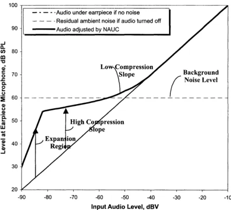
3-2 Plot of how SNSR relates to SNR . . . 3-3 Plot of the NAUC Compression Curve 3-4 Plot of the NAUC Gain Curve ...

A-1 A-2 A-3 A-4 A-5 A-6 A-7 A-8 A-9 B-1 B-2 B-3 B-4

Top Level Simulink Model ....

RMS Detector ... dBO10 Function ... undB20 Function ... Dynamic EQ ...

Dynamic Range Processor (DRP) Dynamic EQ Level Processor . .

NAUC

...

NAUC Level Processor ... Main Function ... Anti-Aliasing Filter ... HPF Filter ... Anti-Zipper Filter ... . . . 16 . . . 17 18 18 . . . .45 . . . .52 . . . 55 . . . .56 80 81 81 82 82 83 83 84 84 86 90 91 93

...

...

...

...

...

...

B-5 NAUC ... 94 B-6 Dewey Filter ... 95

List of Tables

2.1 DSP Spec Comparisons ... ... 28

Chapter 1

Introduction

1.1 Motivations for DSP

Digital Signal Processing (DSP) can provide much functionality that is difficult to implement in an all-analog system. Furthermore, it provides a medium of design that is highly modifiable and customizable. Adding a DSP component to an all analog system allows the designer to rapidly prototype, test and implement many new and powerful algorithms. Also, once the DSP infrastructure has been installed further revisions can be implemented at a pace much quicker than in all-analog.

The goal of this project was to evaluate the usefulness of DSP in noise canceling

headphone applications particularly for use in the Quiet Comfort® 2 (QC2) Acoustic Noise Cancelling® headphones. This evaluation was to serve as a proof of concept to Bose Corporation for future work with DSP in their Noise Reduction Technology Group (NRTG). Supporting a MIT Masters Thesis allowed Bose to explore the po-tential for DSP in this group without having to invest in permanently employing an

engineer.

1.2 Background of the QC2 operation

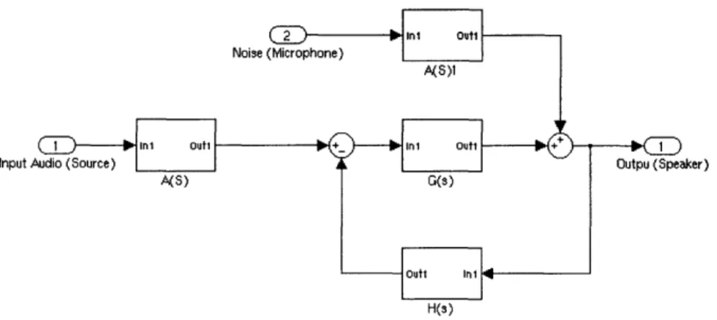
The QC2 currently exists as an all-analog device. It has a power supply that regu-lates an AAA battery to 2.75 V DC (this is a factor we will have to consider when

Input A

Figure 1-1: Analog Block Diagram

choosing our digital components). The audio signal is split into high frequency and low frequency components that are injected into the signal path at different points. There is a forward path that only effects the audio equalization, and there is feedback path that effects both the audio equalization as well as the active noise reduction. Both the forward path and the feedback path are composed of high order active and passive filters (8th order in the feedback compensation).

Figure 1-1 depicts a block diagram of the current implementation. For simplic-ity's sake we are ignoring the frequency splitting of the input audio and visualizing the audio as being injected through one block. Note that the feedback is achieved through the coupling between the speaker and microphone in the ear cup. The trans-fer function between these components is included in the H(s) block.

The active noise reduction peaks at about 20 dB of attenuation. The steady state

power dissipation of the system is about 8-12 mA. If there is a sudden change in noise

levels the power supply can supply up to around 100 mA.

Our goal is to replace, improve, and expand the functionality of the existing analog circuitry. We want to remove any analog circuitry that can be replaced by the digital components we are already installing. We want to improve upon the analog EQ by creating filter topologies that are difficult to generate in analog. Finally, we want to add functionality to the headphones by using clever algorithms that will enable

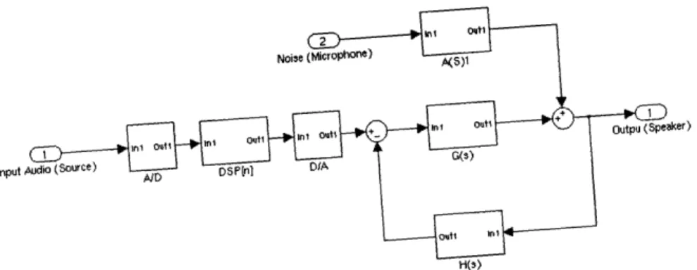
Outpu

Figure 1-2: Digitally Modified Block Diagram

the headphones to adapt in ways that

are difficult to do with limited board

space in

analog.

1.3 Initial Hardware

Modifications

First, we must determine which analog components

do not affect the feedback path.

if the component does not affect the

feedback path, then it can be said not

to affect

the noise cancelation. Our digital circuitry

is going to exist outside of the feedback

loop. Figure 1-2 shows a generalized

block diagram of our digitally modified

system.

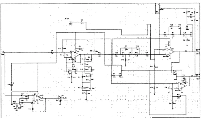
We determined what analog components

could be removed first by simulating

the changes in Spice. We tested to make

sure that the feedback path would not be

changed by more than half a dB at any point

in its contour. These tests resulted in

the modified schematic seen in Figure 1-3.

Once the circuit was modified we then ran

frequency sweep tests on the resultant

circuit to make sure that the simulated

results were accurate. We also simulated

and

tested the resultant analog EQ curve.

The functionality of the components

removed

from the analog forward path must

be replaced in the digital domain. So,

we must

know what the new analog EQ is so that

it may be appropriately adjusted with the

digital EQ. The new analog EQ

curve is shown in Figure 1-4.

Finally, we had to add circuitry in order

to read the signal produced by the ear

cup microphone. Knowing the signal

seen at the microphone allows us to create

Figure 1-3: Modified QC2 Schematic

Frequency (hertz)

active compression algorithms that respond to the background noise level as well as the audio signal level. The QC2 headphone has the benefit of already having a microphone installed to close the Active Noise Cancelation feedback loop. In order to read the voltage from the microphone we must buffer the signal as not to effect the impedance seen at the microphone' output node. We do this with a simple

non-inverting opamp buffer with a gain of 2 (see Figure 1-3). The gain is for prototyping

purposes because the microphone has a lower sensitivity than that of the speaker. If the input impedance of the actual DSP chip is high enough the opamp buffer may not be necessary in the final board level design, but it is important for our evaluation system.

1.4 Algorithm Development

In order to begin building a DSP prototype the designer must first classify the

al-gorithm. That is where we continued our project. We first interfaced our modified

headphones with a Simulink® and Real-Time Workshop®1 floating-point system in order to test initial design ideas (See Chapter 2.1). At this point in the design phase we classified the ultimate functionality of our system. We decided that the system was to firstly provide the ideal static equalization; secondly provide a dynamically adaptive equalization; and lastly provide noise adaptive compression (See Chapter 3). Our implementation of noise adaptive compression was particularly interesting. Prior systems operated by running computationally intensive adaptive filtering to isolate

background noise from signal source based on a microphone signal (a microphone

located in the same environment as the system speaker will have an element of the signal plus the noise) in order to obtain a signal-to-noise ratio. This must be done because the transfer function from the speaker to microphone, in many cases, varies over time and an adaptive filter is necessary to implement a reverse convolution. The noise reduction circuitry, already present in the QC2, leads to a time stable and flat transfer function over the 80 to 800 Hz bandwidth. We took advantage of this

pect to make our compression algorithm as a function of Signal-to-Signal-Plus-Noise (SNSR) thus avoiding much complicated filtering.

1.5 Algorithm Implementation

The next stage in the project was to implement our Simulink design in a functional DSP system. At this stage the actual software that will run on a DSP chip was coded.

Our final choice for our DSP was the Analog Devices ADSP-BF533 (See Section 2.2.1).

This meant that we had to convert our code into a power-sensitive, fixed-point world.

Fixed-point introduced many design concerns that were not apparent while designing

in floating-point. Particularly we had to worry about our systems dynamic range and round off errors (See Chapter 4). Dynamic range became a problem if large gains were applied to the signal and digital clipping resulted. Round off errors were a problem because standard fixed-point notation only rounds to the nearest integer, and

Analog Devices' fractional library only allows for numbers of magnitude less than one. Rounding became a problem in situations such as conversions from a dB boost value to a linear gain. In linear gains we needed values to range from 0 to about 15. Integer values would have been fine at high gains, but at lower gains integer transitions would

be abrupt and unsatisfactory. Fortunately, the ADSP-BF533 is capable of emulating floating-point computation with a fixed-point processor, and many of these problems

were avoided.

1.6 Further Work

Further work would call for code optimization and installation into the QC2 Printed Circuit Board (See Sections 2.3, 2.4, and 5.1). The major optimization step would have been implementing as little floating-point emulation as possible, and then making

design tradeoff choices based on the design complexity and lack of fidelity in

fixed-point algorithms versus the computational intensiveness of floating-fixed-point emulation. We would then have to design a final board-level layout and install our system in the

headphones. At this point we would have a working prototype in its entirety, that would hopefully offer exciting advantages over the current state of the art in analog headphone technology.

Chapter 2

System Design and Development

In this project we designed a Digital Signal Processing (DSP) algorithm for applica-tions on the audio path of the Bose QuietComfort® 2 Noise Cancelling® headphones. The goal was to build a fixed-point system that sampled input audio signals at 48

kHz and processed envelope levels at 2.4 kHz. The system takes as inputs the left

audio signal, the right audio signal, and the microphone signal from the left ear cup, and outputs stereo audio signals to the left and right earcup speakers. The project was designed first on a Simulink rapid prototyping system. Next, the algorithm was ported to an embedded, fixed-point environment. Further work would call for system optimization and installation into the board level circuit of the QC2 headphones. This chapter will cover the steps associated with building a prototype of a DSP system. Our specific design is representative of many problems that are encountered in the prototyping process.

2.1 Algorithm Development

The development of our algorithm was done using Simulink® and Real-Time Workshop®

(RTW)1_{. Simulink is a Matlab® design tool that allows the user to specify signal}

processing systems in block diagrams. Simulink is ideal for building complicated

1Both of these products are made by MathWorks as is Matlab. See http://www.mathworks.com for more information.

systems spanning several layers of abstraction by allowing the user to add

subsys-tems of blocks within blocks. Real-Time Workshop is a design tool which compiles

Simulink systems into executable files. These executables may either run statically, or be actively updated through controls the designer may build into the Simulink system. Our Real-Time Workshop system was made to compile the code to a linux executable. RTW would then transfer this code remotely to a separate linux

com-puter. The linux computer was connected to a 96 kHz, 24-bit RME brand firewire

sound card. The sound card functioned as an Analog-to-Digital/Digital-to-Analog converter (CODEC), the linux computer functioned as the DSP, and the Simulink system functioned as the DSP controller. All together these components created a DSP system that provided extremely fast prototyping capabilities, with high

com-putational power; however, it was not close to board level in terms of size, power

consumption, or limitations on its capabilities.

The Simulink system was designed without regard for fixed-point limitations or power consumption. The rational was to design the best possible system to prove that DSP could provide useful functionality, without worrying about actual imple-mentation. We intended this stage of the project to be a proof of concept. Since the QC2 headphone had never had a DSP system associated with it, we felt that a proof

of concept would be useful. One of our "lessons learned" is that more attention could

have been paid during the design phase to how the final system was to be imple-mented. Simulink has a fixed-point block set and limiting the design to fixed-point

in the Algorithm Development stage could have saved much time in implementing

this algorithm on the final processor (see Section 2.2). At the time, though, we did not know with certainty that the final processor would be fixed-point. In the end this stage served to classify what it was that we wanted the system to do; it did not necessarily provide insight as to how that functionality was to be obtained in a

fixed-point world.

It was during the Algorithm Development stage that we decided exactly how the system was to function. In the initial planning stages we had brainstormed many potential uses for a DSP system. The "dream idea" was to have the DSP aid in active

noise reduction (ANR). Current technology, however, precludes digital ANR because the lag and phase delay associated with current analog-to-digital converters would result in an unstable system. Another notable idea was active loop gain adjustment.

This functionality would allow the system to always remain on the verge of instability, where the loop gain (and hence the noise reduction) is maximized but the system would still barely remain stable. There was also an idea for a compression algorithm where a "night mode" could be turned on to compress the dynamic range of the music

in such a manner to be just audible above the background noise. This function would allow the listener to use music to replace noise as the background environment. In

the end "night mode" was discarded for a subtler form of compression.

During the Algorithm Development stage, we decided to limit the system imple-mentation to three components. First, the system was to replace any analog circuitry that only acted on the forward audio path. This would eliminate much of the audio equalization circuitry. The rational behind this functionality was that by installing the DSP circuitry we are taking up valuable board space and power, and any analog components that could be emulated in digital should be replaced.

The second function of the DSP was to provide an equalization that adapted to the content of the input audio (Dynamic EQ). This came out of the experimental observations that the response of human hearing actually varies depending on the

input level. Studies show (see the curves generated by Fletcher and Munson)2 that

the human ear gets worse at detecting low and high frequency sounds as the signal

level decreases. The fall off for high frequencies is much slighter than that for low

frequencies and was deemed inconsequential. The low frequency loss in response, though, can be quite noticeable. There are several pieces of music that exemplify how noticeable this effect can be when listened to at contrasting loud and quiet

volumes.3 This effect was fixed by implementing a system that first detected the

input level, then added appropriate gain to the low frequency content of the music.

2See http://www.webervst.com/fm.htm[6] for an explanation of the Fletcher-Munson curves

3_{See Saint-Saens Symphony #3 where the organ disappears at low levels. We also listened to}

Holly Cole's "See Clearly Now", Freeze Thaw's "Basia", and Nine Inch Nails' "Piggy" for other examples of low frequency attenuation.

The result of the system was a signal that where the equalization sounds appropriate

at both high and low volumes.

The third and final component of the floating-point system is referred to as Noise Adaptive Upwards Compression (NAUC). Studies in psychoacoustics literature have

shown that signals more than 10 to 15 dB below background noise cannot be heard. This can be a problem in high noise areas especially if the piece has widely varying

dynamic range. If the dynamic range varies slowly, then in order to keep the loud passages bearable and the quiet passages audible the listener may find himself con-stantly adjusting the volume. If the dynamic range varies rapidly, either the quiet

passages will disappear or the loud passages will appear obtrusive.5 In an attempt

to remedy this problem, a research engineer at Bose6 suggested that the audio be

aggressively compressed upwards when below the background noise while leaving it largely uncompressed when above the noise. This was the inspiration for the NAUC

system. To do this we analyze both the input signal level (after Dynamic EQ correc-tion) and the signal level already seen from the microphone in the noise cancelation

feedback loop. We then calculate a wideband gain based on these levels. The goal of the NAUC system was to make sure that the low level inputs are compressed upwards in order to always be audible over the background noise. The user can then set the

level based on the loudest parts of the piece, and the system will guarantee that the quiet passages will be at least audible. Ideally the quiet sections would be compressed the minimum amount to preserve as much of the dynamic range as possible. In prior art, noise adaptive compressor systems implemented complicated adaptive filtering to

isolate the level or spectrum of the background noise sensed by a microphone from the

reproduced audio input signal also present at that microphone. We took advantage of the noise reduction feedback loop inherent in the QC2 headphones to avoid this

4

See Stevens and Guirao (1967), "Loudness Functions and Inhibition" [9]

5

See Respighi's "Pines of the Appian Way" for a piece that begins very quietly and ends very loudly. Set the original volume so that the opening passages are audible in the presence of background noise (e.g., in an airliner or car); by the end of the piece the signal levels will be almost unbearable. See Flim and the BBs' "Tricycle" for a piece with rapidly varying dynamic range. Set the volume such that the beginning passages are at a comfortable level; there will be percussive hits that seem painfully loud.

complicated filtering, which will be discussed in section 3.6.

2.2 Algorithm Implementation

In the algorithm implementation stage the designer must convert the system from an existing rapid prototyping environment, such as Simulink, to an environment that can be implemented in a real product. In our case this meant porting the code from a floating-point, computationally intensive, Simulink environment to embedded DSP code. Our embedded DSP system was coded in C++ for the Analog Devices

Blackfin® ADSP-BF533 EZ-kit LiteTMEvaluation Board7 _{as described later in this}

section. There are many challenges associated with porting an algorithm from a system like Simulink to embedded DSP code. Furthermore, code compiled onto an

embedded DSP chip, especially a low power fixed-point chip like the Blackfin, may

respond differently than it would compiled onto a CPU, or the DSP may not even be able to handle certain code fragments at all.

2.2.1 DSP Selection

We looked at several criteria for selecting the DSP. The most important were

compu-tation capabilities, power consumption, fidelity and dynamic range (bit-count), ease

of portability from Simulink to embedded code, amount of on chip memory, size of the

chip, and any added features that make the floating-point to fixed-point conversion

easier.

The two DSP providers we considered were Analog Devices (ADI) and Texas

In-struments (TI). We chose these companies primarily because they were organizations

with which the Bose Corporation had prior experience. We believed that if Bose em-ployees were familiar with the part we worked with, then they would be able to offer

valuable advice. Each company offers multiple lines of DSP parts. ADI recommended

their low power Blackfin line of DSP, while TI recommended either their low power

7_{see http://www.analog.com/en/epProd/O,,ADSP-BF533,00.html}

for information on this prod-uct.

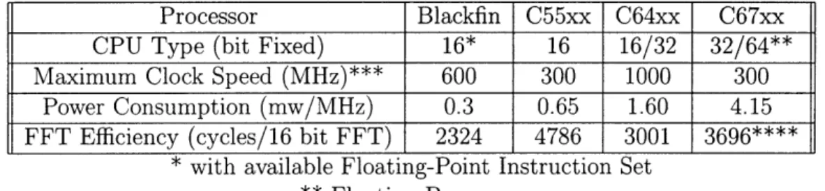
Table 2.1: DSP Spec Comparisons

Processor Blackfin C55xx C64xx C67xx

CPU Type (bit Fixed) 16* 16 16/32 32/64**

Maximum Clock Speed (MHz)*** 600 300 1000 300 Power Consumption (mw/MHz) 0.3 0.65 1.60 4.15 FFT Efficiency (cycles/16 bit FFT) 2324 4786 3001 3696****

* with available Floating-Point Instruction Set ** Floating Processor

*** ADI specifications were listed at mW for a fixed clock speed, and TI

specifications were listed as mA/MHz. The numbers were calculated assuming all processors operated with linear power consumption increases with respect to clock

speed and at a 1.45 mV supply.

**** cycles for an unlabled FFT

C5000 series or their higher performing C6000 series. The C6000 series offered many

performance benefits such as higher maximum clock speeds and a floating-point pro-cessor but the power consumption was too high to make it viable in our application.

For a comparison over the various processors see Table 2.18. With computational

capability and power consumption being our greatest concern it became obvious that

either the ADI Blackfin or the TI C55xx boards would most closely meet our needs.

Many of the TI boards have support from MathWorks for automatically converting Simulink systems to embedded code. This ease of use added some value to the TI boards that may not be obvious through simple benchmark statistics. Upon further investigation, though, we found that there is also third party support that offers

similar functionality for the ADI DSP evaluation boards. This software is called

DSPdeveloperTM and is manufactured by SDL.9

Another statistic not listed in Table 2.1 was the onboard memory. The C55xx

processors offer up to 320 kb of RAM.1 0 The Blackfin offered up to 148 kB of on

chip memory.1 While the TI board offered more maximum storage space, these

8_{Ail data regarding ADI parts was taken from "BF533 Vs TIC55x.ppt" [7] produced by ADI. All}

data regarding TI parts was taken from "boseenrgl21404.pdf" [3] produced by TI. Both number sets

were verified on www.analog.com and www.ti.com.

9

See: http://www.sdltd.com/_dspdeveloper/dspdeveloper.htm

1°See: http://dspvillage.ti.com/

Table 2.2: DSP Efficiency Comparison

Processor Blackfin C55xx Delayed LMS Filter 1.5h + 4.5 2h + 5

Radix 2 Butterfly Kernal 3 5

256pt Complex FFT 2324 4786

Block FIR Filter (x/2)(2 + h) (x/2)(4 + h)

Complex FIR Filter 2h + 2 2h + 4

Max Search 0.5x 0.5x Max Index Search 0.5x 0.5x

Biquad IIR 2.5bq + 3.5 3bq + 2

h # of taps

x = # of samples

two statistics were comparable and both were more than were anticipated for our

design. Having narrowed our choice down to either the Blackfin or the C55xx we could then look at more in depth efficiency comparisons to come to a final decision

(See Table 2.2)12.

After a final analysis of the performance of the two DSP kits the ADI Blackfin appeared to most closely match our needs. This was due to a combination of power consumption, maximum clock speed, and the Blackfin's ability to emulate floating-point computation. We selected the ADSP-BF533 EZ-kit Lite Evaluation board, because it offered the best combination of performance, stability, and support. Also, the engineers at Bose were, in general, more familiar with the ADI parts than the TI parts offering more support possibilities internal to Bose Corporation.

2.2.2

Data Converter Selection

Along with selecting the DSP we also had to choose data converters. Analog-to-Digital Converters (ADCs) are necessary to digitally read both the input music sig-nal and the input microphone sigsig-nal. Also, Digital-to-Asig-nalog Converters (DACs) are necessary to then feed the digital output to the headphone speaker. Combined two-channel Analog-to-Digital/Digital-to-Analog Converters (CODECs) are available

12All numbers taken from

from many companies. We decided that one stereo CODEC for the audio signal

con-version along with one lower speed ADC for the microphone would provide the best solution.1 3 First, we talked to representatives from AKM who offered the AK4555, a

low power 20-bit CODEC that ran at 16 mW. Also, they recommended their AK5355 16-bit ADC that ran at 15 mW. We then talked to representatives from Cirrus Logic

as well as TI. Both companies were in the process of completing low power CODECs,

but they did not have support or evaluation boards available as of yet. This made the

decision to go with AKM relatively straight forward, because we decided the

poten-tial performance benefits of the competitors parts did not outweigh the advantages

of having a well supported and tested device.

2.2.3

Embedded Design

There can be many difficulties encountered in porting a floating-point algorithm from

a rapid prototyping system such as Simulink to embedded code on a functional,

fixed-point DSP. The designer now has to worry about what functions are native to the embedded language (C++ or Assembly in our case); the designer must worry about problems associated with fixed-point calculations; the designer must worry about how

many computations the system is using on any given sample; also the designer must

worry about how much memory is used in order to store the algorithm.

Rewriting the algorithm in C++ can be more challenging than it may seem ini-tially. There are several built in functions in Simulink that may not be native in the C++ environment. One particular difference encountered in our design was that our

Simulink model was originally designed as a streaming implementation and many of the ADI libraries called for data to be given in blocks. A streaming implementation processes the input in a sample-by-sample methodology while a block processing

im-plementation collects some predetermined number of samples and runs the algorithm on the block of data. This is analogous to the "Windowing" associated with many signal processing algorithms. Block processing algorithms usually ignore data

asso-13The microphone only operates on the envelope domain of the signal for level processing. For information on this see Chapters 3 and 4.

ciated with previous blocks leading to artifacts around the beginnings and ends of blocks when running IIR and FIR filters. The advantage of using a block processing implementation is that it is usually less computationally intensive. Let us look at a generic filter as an example. In the streaming methodology the DSP must load the

coefficient values out from memory every sample cycle. In a block implementation

the system must only load these values once per block. As a result there is less set up computation. In Simulink there are native functions for buffering and unbuffering samples into blocks and the samples into blocks. In C++ something like this must

be coded by the designer. In the end we experienced difficulty getting the ADI block

implementations of IIR filters to work properly in our system, so custom sample-by-sample IIR filters had to be coded. In Simulink there are standard blocks that will

run IIR filters on either a block of data or a single sample. In our embedded code

custom biquads were hard coded. Each biquad operated via[8]:

x[n2] = x[n

1];

x[n - 1] = x[n];

x[n] = input;

y[n - 2] = y[n- 1];

y[n- 1] = y[n];

y[n] = bo * x[n] + b * x[n- 1] + b2* x[n - 2] - a * y[n - 1] - a2 * y[n - 2];

The biquad example is also perfect for illustrating some of the difficulties in

equaliza-tion filter4 called for coefficients of: a₀ = 1 a, = -2 a2 = 1 b = 0.93461 b2 = 1.30045

Standard fixed-point convention only allows the programer to operate on integers. Rounding these coefficients to the nearest integer would cause a vastly different filter.

The ADI libraries, however, have conventions for specifying fixed-point numbers that all range from -1 to 1. A binary value of all 's (listed from MSB to LSB) is constructed

as:

-2 0+ 2-1 + 2-2 2-3... + 229 + 2-3 0 + 2-31

This allows us to account for values less than 1 in our designs; however, it does

not provide the programmer with a method for accounting for numbers greater than 1 with a fractional component. To design fixed-point filters we must redesign our

biquads to only use coefficients less than 1. To do this we first divide each coefficient

by the lowest multiple of 2 greater than the largest coefficient value (multiples of 2 are used so the the divide may be accomplished using simple binary shifts) in our

case this value was 2. This reduces each coefficient to a value less than 1. Our output equation is now:

y[n]

_{[] = -- * x[n]}

_{+ ix[n-1] +}

2

* x[n - 2]

_ , y[n -1] - -2

, y[n -2]

2 2 2 2

This would be a rather straight forward equation except for the n term. We cannot

simply divide y[n] by two because we need to get access to what y[n] actually is in

4_{We refer to the ideal equalization curve for the QC2 as the Dewey after the engineer who}

order to generate the delayed output terms. In order to accomplish this we use:

Y[n]

frac

=

* x[n

+

x[n-2]-

*

]

,

y[n-1]-

2

* y[n-2]

2 * y[n]frac = y[n]

and then feed this y[n] back into the delay line. The multiply by two may also be

accomplished with a simple binary shift. In the end we used floating-point emulation in order to accurately generate the Dewy filters (see Section 2.2.1 for information on the Blackfin's floating-point emulation). Even though emulating floating-point is relatively inefficient in terms of computation the fidelity it added was deemed appropriate for an initial step in completing an embedded prototype.

Fixed-point processors also limit the instruction sets that the C compiler is able

to use. Many operations are only available as floating functions. The two examples of operations like this that affected our design were the log and power functions. In

order to go from linear to dB space one must run a loglo on the linear input according to the dB20 equation:

OutputdB

=

and to go from dB space back to linear one must compute a power function according to the undB20 equation:

InpUtdR

OutputLinear = 10 20

These functions, though, will always return either floats or doubles (extended

preci-sions floats). Some implementation of these functions typically much unavoidable if

the programmer wants to use algorithms acting in the dB domain unless a logarithmic tapered ADC is used. We can use floating-point emulation in order to generate these functions. The loglOf and powf functions are floating-point functions that can ac-complish the desired computation. The powf operation, however, seemed to overwork our processor and resulted in a "fuzzy" sounding output. In fact, if the operation

was anywhere in the code, even if it was not affecting the output, the output would

still be fuzzy. The probable explanation for this effect is that the powf function, being generated through floating-point emulation, was too computationally intensive for our fixed-point processor to compute in the time it took to run one sample. As

a result samples were lost and a lower fidelity output was heard. A similar effect

was heard if the printf operation was used (displays data values on the terminal)

in which case almost every output sample was lost and only fragmented blips were

heard. The loglOf function, though, emulated without resulting any any lost samples

or "fuzziness".

One possible solution would be to use a Taylor series in order to approximate

these functions. Another solution would be to remap any dB based operations into linear space. The later was the first solution that we attempted. For the Dynamic EQ this resulted in a function that had an InputC term in it (where C is some constant). In order to obtain the accuracy and output range needed we used a 5 term Taylor series that was expanded around multiple regions. We would check the input and

run a different 5 term Taylor Series depending on its value. Another solution was to

use the loglOf function in order to get into dB space, and then use a Taylor series to return to Linear space. This Taylor series takes the form of:

* ioa * (X + ln(a)2 * 10a

OutputLinear = 10a

+ ln(a)

₊

_(x

_a)

ln(a) * lOa 3 ln(a)4 * o10a

3!

3!

* (x

-

a) +

4!

* (x

a)'

Where a is the point about which we are expanding. Converting back from dB space

to a linear gain via a Taylor expansion of the undB20 equation resulted in a fairly accurate output with only having to Taylor expand about a singule point. Also, it is computationally simple enough to result in no dropped samples. We pre-computed

many of the factors so that they were not actually have to be calculated by the processor. Instead they are stored as coefficients to the (x-a) terms.

We are still left with the problem of fractional numbers that we encountered in our filter design problem. In our application many of our coefficients are non-integers

greater than 1, and even if the coefficient was purely fractional the (x-a) term may be a non-integer greater than 1. In order to use fractional arithmetic both inputs

must have amplitudes less than 1. It would be possible to design a more complicated

system that used only integer and fractional multiplication and addition, but floating

emulation was deemed sufficient for our purposes. This resulted in a clean, accurate

output.

This operation is an example of a case where a floating-point processor may one

day be lower power than a fixed-point processor. Fixed-point processors will always be lower power than floating-point processors in terms of mW/MHz, but accurately computing this Taylor expansion would use fewer clock cycles with a floating-point processor than it would with a fixed-point processor even without using floating em-ulation.

A final concern to keep in mind at this point in the design stage was the amount of memory being used. If the internal memory were to be exhausted external memory would have to be installed. This would require more board space to be allocated to DSP components in the final design, and external memory accesses are power intensive. The VisualDSP++® Lite software (the software that comes with the EZ-Kit Lite evaluation board for compiling C++ or Assembly code onto the DSP) limits the programmer to 22 kB of storage space. This amount of memory was quickly

exhausted. Once a full VisualDSP++ license was obtained (free for 90 days with the ADI Test Drive program)1 5 and full access to the 148 kB of on chip memory was

available, there were not any problems with memory limitations.

2.3 Optimization

Once the basic design is operational, the designer must take into consideration all the ways the system can be optimized. The first step is to quantify how much power is being used. The designer can do this by setting the clock speed of the DSP processor.

The lower the clock speed the less power is being used by the chip (See Table 2.1 for

statistics on power as a function of clock speed). If the chip cannot be clocked at the desired clock speed (this will most likely be apparent by a lossy signal where samples

are dropped), then the algorithm must be optimized to reduce the amount of power consumed.

The most straight forward way to optimize the system would be to reduce or remove instances of floating-point emulation. If we were to rebuild our filters in the fractional method mentioned earlier, and redesign all floating-point operations as combinations of integer and fractional operations, then there would be a good savings

in power costs.

The second way power consumption can be reduced is to switch from a streaming to a block processing implementation. As mentioned earlier block processing reduces setup costs in initializing computation. However, artifacts can be created and we may not get as true a response as we would with a streaming implementation. The designer must take these types of considerations into account. The longer the block being processed the truer the result will be and the more setup computations will be reduced, but at the same time the the amount of memory used in delay storage will increase and the amount of computation that must be done when the block executes increases. If the block becomes too long the system may not have time to fully compute it in a sample-cycle and the data computation may have to become asynchronous with sampling. By asynchronous computation we mean that the we would collect a new block and output an old block synchronously with the

sample-clock, while the current block is processed on it's own. Also, the designer can utilize

tricks with overlapping neighboring blocks in order to eliminate edge artifacts, but

those techniques result in there being less savings in setup costs for a given block

length. Finally, if the block becomes too long delays that are unacceptable may occur, because the input to output delay must be at least one block length (in this manner

2.4 System Installation

Once the algorithm has been verified and optimized we can build the final system.

If we had multiple engineers working on the project the hardware design would have been conducted in parallel with the software work. In our case we had a single

engineer working, so the hardware design was not completed. This stage consists of PCB layout design, power supply design, and interfacing the digital components. For relevance to this project we are assuming that we are starting with an already existing PCB board that must be redesigned to fit our new needs.

The first thing we did was remove all of the unnecessary parts in the analog portion of the circuit that were only contributing to the forward path equalization. There were a handful of capacitors and resistors that did not effect the loop gain but affected the forward path. First, the effects of removing these parts were simulated and then they were verified in lab tests to make sure that the feedback bath (and hence the noise cancelation) would not be altered. The effects of these components were taken into account when we designed our Digital Dewey filter to provide the correct audio equalization. Removing these parts freed up some amount of space for

the new digital components.

The AKM AK5355 ADC operates on power supplies ranging from 2.1 to 3.6 V.

The power supply on our board is 2.75 V so we do not need any modifications to obtain

new voltages for this part.1 6 There is good documentation for how to configure this

part in its data sheet17_{. We see that adding this part will call for the addition of 8}

capacitors as well as the added board space required for the part itself. The Controller and Mode Setting blocks would be control pins from the DSP chip.

The AKM AK4555 CODEC operates on power supplies ranging from 1.6 to 3.6

V. So, once again we would be able to operate this part without any power supply modifications. Like the ADC this part's configuration is documented in its application

16For a truly power optimized system we would want to include circuitry to allow the digital components to run at their lowest allowed supply voltages. The lower the supply voltages the lower their power consumption will be

notes.1 8 Installation of this part requires 7 additional capacitors and 2 additional load resistors. The components already installed in the system may be adequate for the load resistors, and it is suspected that these parts are not necessary. Again, the Controller and Mode Control blocks would be control pins from the DSP chip.

The BF533 is a significantly larger chip and more care has to go into installing it. It comes in a mini BFG package and the traces to and from the chip will require that much care goes into the layout design. Our current PCB board has four layers, and

it may be worth considering adding more trace layers to make for easier design of the

wiring. This chip has control pins that interface with both the CODEC and the ADC. It also has I/O pins that must be able to read the digital data from the CODEC and ADC and then feed the digital outputs back to the stereo CODEC. Bypass capacitors may be necessary on the supply rails as well to make sure that digital noise is not injected back into the analog signal (these capacitors will be similar to those called for

by the converters). The DSP chip calls for two power supplies; the first is the external supply voltage can range from 2.5 to 3.3 V the second is the core voltage which can

range from 0.8 to 1.2 V. Fortunately, the Blackfin has an on-board voltage regulator so the core voltage can be generated from the external voltage source combined with a few discrete components (as documented by the application notes). So, again we will be able to run this chip off of our currently existing supply voltage.

2.5 Summary

In summary we find that there are several concerns that we must be aware of in the process of developing a prototype. It is useful if we can be aware of our final design space while we are trying to design the functionality in the algorithm. If we

are not aware of our final design space during the preliminary design, then there are several design adaptations that we can expect to make. Design efficiency, fixed-point limitations, sampling methodology tradeoffs are aspects that we must be aware of.

Ideally this project would have been conducted with at least two engineers so

8

that the hardware and software designs may be conducted in parallel. The work flow in the case of multiple engineers would be: algorithm design and initial hardware modifications; embedded code and layout design; software optimization and system

installation. In our project, however, we only had a single engineer. The algorithm

design and initial hardware modifications were still done in parallel, but embedded coding and layout design both require large amounts of attention and the layout would have been designed after the embedded code was made.

Chapter 3

Simulink Algorithm

In this chapter we detail the algorithm as it exists in its Simulink, floating-point form. This chapter also documents the theory and rationale behind the design of the various operations as applied to the overall DSP design. Ideally a fixed-point system would be identical to the algorithm, as described below, in terms of functionality

even though it would be different in implementation. As stated in Section 2.1 the

Algorithm Development stage in DSP prototyping is to demonstrate functionality, as this chapter details for our system.

3.1 Input Adjustment

The inputs to both the right and left channels are scaled by a gain factor of 5.8. This serves to offset a constant adjustment associated with the analog-to-digital conversion.

This scaling results in a 1 Vrms input yielding a value of Vrms at the input level

detector. In a computationally efficient version this gain would be omitted and the constant difference would be taken into consideration in the level processing stage.

After the initial scaling the inputs are unbuffered. The original signal is sampled

in frames of 256 samples, a buffer of 50 ms, and 10 ms Period/Fragment. For our

floating-point, computationally intensive, implementation we want to process the data

via a streaming methodology, so we first unbuffer the signal to obtain sample per

3.2 Dynamic EQ Level Detection

The level detection for the Dynamic EQ is run on a combination of both the left and right channels. Due to the fact that in music the left and right channels tend to be in phase we were able to obtain the signal of interest by simply averaging both channels.

A more accurate result would be obtained by running individual RMS detections on

both the left and right channel, but this is computationally inefficient and summing and scaling the two audio signals provides an accurate representation. The purpose of

looking at a combination of both channels rather than a single channel is to guarantee

that the system will react to stereo effects that are present in only one channel. To

save on more computation the divide by two adjust could be combined with later level adjustment scaling.

We then run our level detection in the envelope domain of the audio signal. Since, the envelope domain operates at a much lower frequency than the audio spectrum we are able to first down-sample to 2400 Hz. Our decimation lowpass filter consists of an 11th order Chebyshev type II filter. The passband frequency is 800 Hz and the

stop band is 1200 Hz with 80 dB of attenuation. We used a Chebyshev type II filter

because it has greater attenuation per order than a Butterworth filter, in exchange it has ripple in the stopband. However, for audio purposes we are only concerned with the passband, and ripple in the stopband is acceptable. We did not want to use a Chebyshev type I or an Elliptical filter because they both have passband ripple. For a less computationally intense filter we could adjust the parameters so that the the stopband frequency would be above 1200 Hz, and lower the attenuation to only 60

dB.

After anti-aliasing the audio signal is down-sampled to 2400 Hz. The down-sample

is made up of a simple divide by 20 decimation, followed by a zero order hold. The

zero order hold is necessary because the system clock still operates at 48 kHz. The RMS detection operates under a feedback degeneration topology. Firs,t the input is squared. The current output is delayed by 1 sample to save the previous output. The previous output is then multiplied by a scaling factor and summed

with the current output. This detector serves as an approximation of a weighted integration. We adjust the scaling factors to give our system a fast attack and a slow decay. This allows us to quickly detect large increases in level but not jump up and down during quick, quiet segments. The decay constant is decided by comparing the current; output with the previous output. If the current output is greater than the previous output we use the fast attack constant, otherwise we use the slow decay constant. The result of the comparison is delayed by one sample for stability purposes. The fast attack constant is 0.9995, and the slow decay constant is 0.99999.

These coefficients result in rise and fall times that are similar in linear space. Our gains, however, are applied linearly in dB space. Our RMS output ranges from 0 to

1 Vrms2 (because we never actually take the root). This then needs to be converted

into dB units, which we obtain via the equation:

OutputdB = 10 * log(InputLinear)

We use the factor of 10 rather than 20 as an alternative to taking the square root in the RMS. This can range from negative infinity to 0. We then add a factor of 110 in order to obtain units of dBSPL (dB Sound Pressure Level). For practical

considerations we will say a "quiet" input corresponds to a dBSPL level of 20 and a "loud" input corresponds to a dBSPL value of 110. For our practical rise and fall

times (in dB space) we will consider the times it takes to go from a steady state quiet

level to 90% of the difference (20 to 101 dBSPL) and a steady state loud level to 10%

of the difference (110 to 29 dBSPL). For the time being, imagine the linear output of the RMS detector increases and decreases linearly with respect to time. First,

imagine that the linear output of the RMS detector increases from 0 to Vrms2 in

one second (this is a contrived situation). The dBSPL level will reach 20 dBSPL at

1 * 10- 9

seconds and 101 dBSPL at 0.126 seconds, yielding a dB rise time of 0.126 seconds. Now imagine that the output of the RMS detector fall from 1 to 0 Vrms2

in _{second. The dBSPL level will reach 110 dBSPL at 0 seconds and 29 dBSPL} at 7.9 * 10-' 9 seconds. We see that if we view the output of the dB conversion as a

linear function the steady state to 90% rise time is an order of magnitude less than the steady state to 10% fall time. Because our gains are applied as linear functions

of dB we can treat our rise and fall times in this way. In terms of dB space we should expect to see a difference in rise and fall times of about one order of magnitude not accounting for linear differences in the attack and decay of the RMS filter.

Measured results show that the RMS rise and fall times are on the order of a couple seconds in linear space. The rise time in dB space was measured to be a little under a second, while the fall time in dB space was measured to be on the order of

10 seconds. This is consistent with the previous paragraph also taking into account the minor differences in the attack and decay coefficients. The output of the RMS

detector is scaled by 0.0005 in order to preserve the 1 Vrms in leading to 1 Vrms2 out

of the detector. To save computation this scaling along with all the other previously mentioned scaling factors would be merged into the dB to dBSPL conversion.

The output of the RMS detector is then converted to dB units. This is done with

a dBO10 conversion (dBO10 instead of dB20 is used because we have already squared

the input, thus we have combined the root part of the RMS detection and the dB

conversion into one stage as mentioned above). After the initial dB conversion we

add a factor of 110 to convert dB units to dBSPL (dB sound pressure units) units. This is because 1 Vrms applied to the speaker yields a 110 dBSPL signal in the ear cup of the headphones. This is the stage where all the previous constant gain stages

could be merged to optimize for efficiency.

3.3 Dynamic EQ

3.3.1 Theory of Dynamic EQ

It is commonly known that the response of a human ear is level dependant. The Fletcher-Munson curves (See Figure 3-1)1 showed that furthermore the human ear's sensitivity decays faster at low frequencies than at mid-band frequencies as the signal

i I111 ! I!!! ,J--P-4-J

I I I IlilJE

I

_{[ IllllI~'q LlfF"-W.ICT1}

20 50 100 500 1000 5000 10.000 20k

Fequefcy h.

Figure 3-1: Fletcher-Munson Curves

level is lowered. It also showed that human hearing responds in a similar manner

to high frequencies. This high frequency response is much less severe than the low

frequency response so compensating for this has been deemed unnecessary. Older hi-fi systems addressed this with a switchable loudness control that added a fixed bass and possibly treble boost that approximated the inverse of the Fletcher-Munson curves at some predetermined low level relative to a high level; more sophisticated systems adjusted this boost in response to the volume control setting. Our system uses digital level detection and gain adjustment to provide a more natural and effective bass boost than that which was provided by the loudness control.

The Dynamic EQ is fundamentally a block that takes a signal level as input and

then computes a gain value. This gain is mapped onto a two-segment piece-wise linear function in order to approximate an asymptotic function. If the the level drops bellow a certain threshold the gain increases from 0 with a certain slope. Once the input then drops below a second threshold the gain slope increases to the second piece-wise component slope. If the signal falls too low, though, the gain will remain

CtI 41

its maximum value as to not apply overly large gain values when the input is turned

off.

The two-segment piece-wise linear function is generated by feeding the RMS

dB-SPL level into two parallel Dynamic Range Processors (DRP). The DRPs function to compute a linearly increasing boost, in dB units, from an input. Each DRP is

configured with a max gain (dB), a slope (dB/dB), and a breakpoint (dBSPL) that

is the maximum input that will yield a gain. The actual parameters are Bose trade

secrets and have been omitted from the report. One of the DRPs is configured to

start at our actual breakpoint, and hit its maximum value when we want the second piece of the function to begin. The second DRP begins to apply gains when the first unit reaches its maximum gain output value. The output of the two DRPs are then summed together. This means that the max gain of the second DRP is set equal to our desired max gain minus the max gain of the first DRP.

The output from the DRP's is then converted to linear units. This is done simply by the equation:

Output = 10 IrPu '

The result is then reduced by one. One way of justifying the reduction of one is

that a boost of 0dB maps to one through the undB, but we want a gain of zero. An alternative way of looking at this is that this gain is going to be applied to the low frequency components of our signal and then summed back to the wideband. The

wideband, however, contains all of the low frequency information as well, so we must subtract one to have a gain of 1 in the overall system. In short terms the undB gives us a total gain, but what we really want is a boost above the original signal.

3.3.2 DRP Operation

First, the input is subtracted from the breakpoint value. The result of this is then sent through a max function with 0. This basically means that if input is greater

if however the input is less than the breakpoint then the difference is passed. This difference is then multiplied by the slope to give us the amount of boost to apply.

Boost = (Breakpoint- Input) * slope

The result of the multiplication is then sent through a min function with the maxi-mum gain value. Thus if the gain to be applied is greater than our maximaxi-mum desired value, then we will simply pass the maximum value to the output.

3.4 Up sampling

The gain value then must be up sampled back to 48 kHz in order to be applied it to the audio signal. First, the gain value is zero-padded by a factor of 20. Then a

holdvalue function must be implemented in order to maintain the gain value during

the zero padded sections. Since we are only concerned with gain levels, we can simply

hold the DC value and then lowpass filter to smooth the transitions, rather than running a rigorous interpolation function. The hold value function works by looking for edges of the input. If an edge (corresponding to a sample) is seen then the input is passed to the output. If an input is not seen then the output is fed back and sent again. This results in the output only changing when gain samples are sent, and then holding value during the zero padded sections, similar to the built in zero order hold. To further smooth the result the output could be passed through a lowpass smoothing filter (anti-zipper filter) to smooth the transitions, but since the gain only acts on the bassband, sudden changes are not significantly noticeable

3.5 Dynamic EQ Level Processor

The output of the Dynamic EQ is calculated by multiplying the gain value by a filtered version of the input. This filtered signal is then summed back in with the wideband signal to yield the original audio plus a boosted component. The filter used is a single biquad section; the filter parameters were determined by extrapolating from listening

tests done during the design of the Bose Wave® Music System. Both the filter parameters and the gain calculation parameters were extracted from these studies. This level processing is run individually on both the left and right channels, but with

the same gain value for each channel.

The signal that was filtered to generate the bass boost only comes from the left

channel. This is because most music at the low frequencies processed by the Dynamic

EQ are monaural. A more accurate level processor would operate individually on each

channel, but this would add too much complexity to offset the added value.

3.6 Noise Adaptive Upwards Compression (NAUC)

[Patent Pending]

3.6.1 NAUC Theory of operation

Studies show that audio with a signal-to-noise ratio less than -10 to -15 dB is

fun-damentally not present to the listener; this effect was discussed in Chapter 2.1 when we first introduced the concept of the NAUC. Fundamentally, the NAUC guarantees

that an input signal will always be above this signal-to-noise threshold. To do this

the system looks at the input signal, compares it to the signal level seen at the

mi-crophone which is already in place for the closed loop active noise cancellation, and

calculates an amount of gain to apply to the signal. On the surface this operation

seems very similar to that of the Dynamic EQ; however, operating on the wide band as well as making a decision based both on signal-level and microphone-level adds complexity.

The NAUC could be used in a few different ways. One major use for the NAUC could be for music with very wide dynamic ranges over a long period of time. Respighi's

"Pines of the Appian Way" for example starts very quietly, but by the end is

over-bearingly loud if one leaves the volume level set only at the level that is needed to

make the beginning audible. The NAUC would allow the user to initially set the