Adaptive robust optimization with applications in inventory and revenue management
Texte intégral
Figure

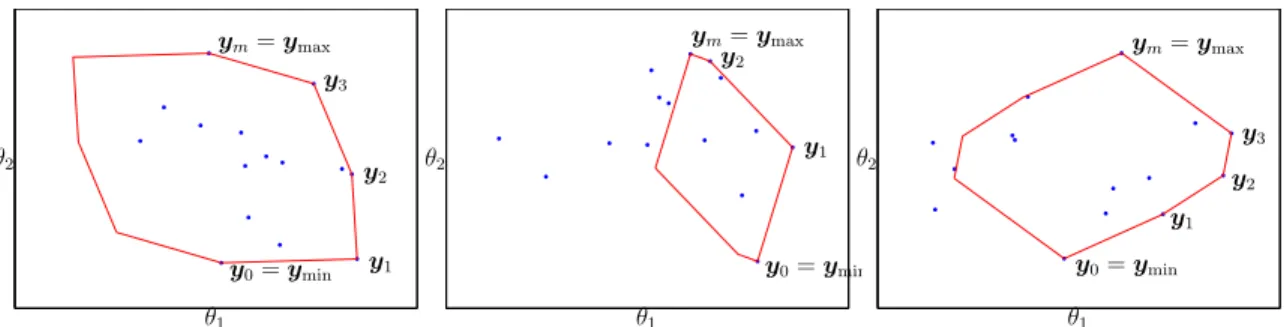
![Figure 2-4: Trivial cases, when zonogon Θ lies entirely [C1] below, [C2] inside, or [C3]](https://thumb-eu.123doks.com/thumbv2/123doknet/13864148.445788/48.918.133.780.511.664/figure-trivial-cases-zonogon-θ-lies-entirely-inside.webp)


Documents relatifs
Molecular analysis of the anaerobic sludge obtained from the treatment plant showed significant diversity, as 27 different phyla were identified.. Firmicutes,
Analyses of the Cardiovascular Risk Factors, Aging, and Incidence of Dementia (CAIDE) study have shown raised midlife cholesterol levels greater than 6.5 mmol/L to be
Marijuana consumption 14 42 Alcohol consumption 25 76 Suicide attempt + marijuana 1 3 Suicide attempt + alcohol 11 33 Dependency 11 33 Dependencyto alcohol 10 30 Dependency to
Table 4 further shows that logistic models including all factors reveal that the main covariates for reporting refusal were having sustained violence (adjusted OR 2.68),
This is because clinical trial endpoints must be able to capture both patient decline and treatment efficacy, and cognitive decline is much more difficult to capture within one year
It goes without saying that the idealist German school (represented by the philosopher Wilhelm Dilthey) believes that human studies are as unexplained as human
Résultat d’une importante enquête ethnogra- phique dont de larges extraits sont insérés sous la forme d’inter- views, c’est aussi par le regard de la
Cet ouvrage touche particulièrement le laboratoire Les Afriques dans le Monde parce qu’il appartient au champ des études africaines bien sûr mais également parce
