Advanced response matrix methods for full core analysis

(1)

Advanced Response Matrix Methods for Full Core

ARCH4VEZ

Analysis

_MASSACHUSTS _INSTffWE

OF TECHNOLOGY

by

APR

08 201k

Jeremy Alyn Roberts

LIBRARIES

B.S./M.S. University of Wisconsin

-

Madison (2009)

Submitted to the Department of Nuclear Science and Engineering

in partial fulfillment of the requirements for the degree of

Doctor of Philosophy in Nuclear Science and Engineering

at the

MASSACHUSETTS INSTITUTE OF TECHNOLOGY

February 2014

Massachusetts Institute of Technology 2014. All rights reserved.

Author ...

Department of Nucl

r

fence andEngineering

eptember 23, 2013

C ertified by ...

...

Benoit Forget

Associate ProfessorLf Nuclear Science and Engineering

Thesis Supervisor

Certified by ...

...

Kord Smith

KEPCO Professor of the Practice of Nuclear Science and Engineering

Thesis Reader

Accepted by ...

...

Mujid Kazimi

(2)

(3)

Advanced Response Matrix Methods for Full Core Analysis

by

Jeremy Alyn Roberts

Submitted to the Department of Nuclear Science and Engineering on September 23, 2013 in partial fulfillment of the

requirements for the degree of

Doctor of Philosophy in Nuclear Science and Engineering

Abstract

Modeling full reactor cores with high fidelity transport methods is a difficult task, re-quiring the largest computers available today. This thesis presents work on an alterna-tive approach using the eigenvalue response matrix method (ERMM). The basic idea of ERMM is to decompose a reactor spatially into local "nodes." Each node represents an independent fixed source transport problem, and the nodes are linked via approximate boundary conditions to reconstruct the global problem using potentially many fewer

explicit unknowns than a direct fine mesh solution.

This thesis addresses several outstanding issues related to the ERMM based on de-terministic transport. In particular, advanced transport solvers were studied for applica-tion to the relatively small and frequently repeated problems characteristic of response function generation. This includes development of preconditioners based on diffusion for use in multigroup Krylov linear solvers. These new solver combinations are up to an order of magnitude faster than competing algorithms.

Additionally, orthogonal bases for space, angle, and energy variables were investi-gated. For the spatial variable, a new basis set that incorporates a shape function char-acteristic of pin assemblies was found to reduce significantly the error in representing boundary currents. For the angular variable, it was shown that bases that conserve the partial current at a boundary perform very well, particularly for low orders. For the deterministic transport used in this work, such bases require use of specialized angular quadratures. In the energy variable, it was found that an orthogonal basis constructed using a representative energy spectrum provides an accurate alternative to few group calculations.

Finally, a parallel ERMM code Serment was developed, incorporating the trans-port and basis development along with several new algorithms for solving the response matrix equations, including variants of Picard iteration, Steffensen's method, and New-ton's method. Based on results from several benchmark models, it was found that an accelerated Picard iteration provides the best performance, but Newton's method may be more robust. Furthermore, initial scoping studies demonstrated good scaling on an

0(100) processor machine.

Thesis Supervisor: Benoit Forget

(4)

(5)

Acknowledgments

I want first to express my sincere gratitude to my advisor, Prof. Ben Forget, for his

advice and guidance over the years. This work was influenced significantly by his own graduate work, and the freedom I've had to explore the topic and others has been an essential and much appreciated part of my time here.

I would also like to thank my thesis reader, Prof. Kord Smith. The practical, real world experience he brings to the classroom (and elsewhere) is invaluable, serving as a constant check against the somewhat more abstract mathematical approach I under-took for this research.

Additionally, Prof. Michael Driscoll and Prof. Emilio Baglietto have my appreci-ation for serving as an additional committee member and chair, respectively, and for providing valuable suggestions to improve the present (and future) work.

My time and education would not have been the same without the many fruitful

discussions I've shared with friends at the office. I'll miss the morning walk-by chat with Bryan, the office chats (about violins, 100+ digits of 7r, etc.) with Nathan, the many chats with Matt where I had to remember why class Foo did that one thing that one way', the (one-way) chats (rants, really) with Gene, the chats where I promised Paul that I would actually contribute to OpenMC (on the radar, I swear), the nerdy transport chats with Lulu, the greedy chats with Carl, the homework chats (venting sessions) with 106 students, and any of the many other chats I've been fortunate to have.

At home, the chats involved lots of neutrons going in and out of the box, but were just as fruitful, and for that I owe my wife Sam all the love in the world. I might also add I owe it to little Felix-to-be for providing a very big impetus to complete this work sooner than later.

I would also like to acknowledge the Department of Energy and its Nuclear Energy

University Program for the graduate fellowship that partially supported the first three years of this work, giving me flexibility to pursue a topic of interest to me.

(6)

List of Figures

2-1 Discrete ordinates discretization in 2-D Cartesian coordinates. The shaded

region denotes cell (i, j). . . . . 27

2-2 MOC tracking of a 2-D Cartesian mesh using Gauss-Legendre points. . . 32

2-3 Sample code for construction of loss matrix. . . . . 39

4-1 Three group transport operator sparsity pattern. . . . . 65

4-2 Spectrum of A and the DSA-preconditioned spectrum. . . . . 66

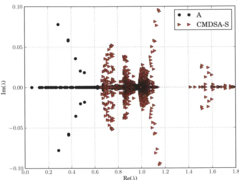
4-3 Spectrum of A and the CMDSA-preconditioned spectrum. . . . . 67

4-4 Spectrum of A and the CMDSA+ S-preconditioned spectrum. . . . . 68

4-5 Spectrum of A and the TC+CMDSA+S-preconditioned spectrum. . . . . 69

4-6 Seven group C5G7 assembly. . . . . 70

4-7 Comparison of flux and pin fission rate error norms as a function of successive flux difference norm. . . . . 72

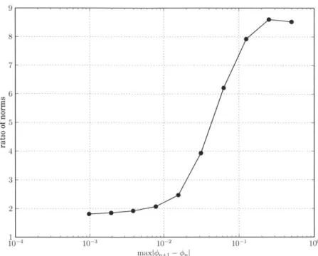
4-8 Ratio of pin fission rate error norm to flux error norm as a function of successive flux difference norm. . . . . 73

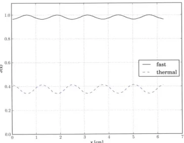
5-1 Fast and thermal group partial currents. . . . . 82

5-2 Fast and thermal eigenspectra of U0 2-MOX minicore. . . . . 82

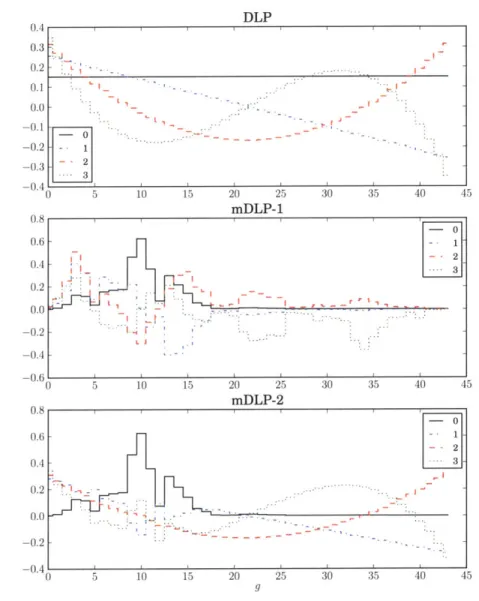
5-3 DLP and mDLP basis sets for 17 x 17 UO2 assembly. . . . 83

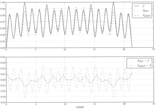
5-4 Comparison of fast group expansion and errors. . . . . 84

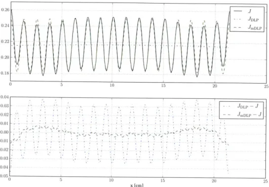
5-5 Comparison of thermal group expansion and errors . . . . 85

5-6 Slab reactor schematics. . . . . 93 5-7 Absolute relative error in eigenvalue and maximum absolute relative

(13)

5-8 2-D Quarter Assembly ... . 95

5-9 Absolute relative error in eigenvalue, and average and maximum ab-solute relative error in fission density as a function of angle order for several expansions. . . . . 96

5-10 Three region, mixed energy slab. . . . . 98

5-11 1-D pin cell lattice schematic. . . . 101

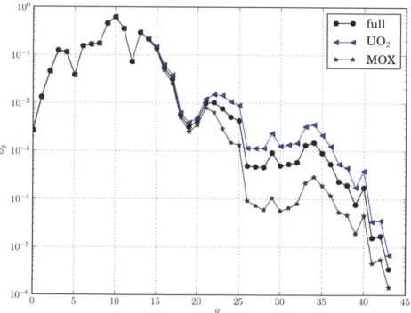
5-12 Critical spectra of the full lattice and the U0 2 and MOX pins. . . . 101

5-13 Comparison of DLP and modified DLP energy bases. Each basis is or-thonorm al. . . . 104

5-14 Comparison of eigenvalue errors for various energy bases. . . . 105

5-15 Comparison of pin fission rate errors for various energy bases. . . . 105

6-1 Dependence of asymptotic error constants on A for several slab widths. 118 6-2 Dependence of asymptotic error constants on node width A. The solid line represents 1-D diffusion, and the markers represent 2-D diffusion. The dashed line corresponds to 1-D transport. . . . 119

6-3 Dependence of asymptotic error constants on node width A. The dashed line represents the two group case. The solid line represents the same problem homogenized to one group using the reference two group solu-tion . . . 12 1 6-4 Two group and one group IAEA convergence. . . . 122

6-5 Three group and one group assembly convergence. . . . 123

7-1 Representative current eigenspectra for the IAEA problem. In both cases the maximum modulus along the imaginary axis is e P 0.54. . . . 127

8-1 Absolute relative eigenvalue error for the 2-D IAEA problem as a func-tion of residual norm tolerance for several spatial orders . . . 137

8-2 Maximum absolute relative assembly power error for the 2-D IAEA prob-lem as a function of residual norm tolerance for several spatial orders. . 138 8-3 Absolute relative eigenvalue error as a function of spatial order. . . . 139

(14)

8-4 Maximum absolute relative assembly power error as a function of spatial

order.. . . 140

8-5 Comparison of Picard acceleration schemes for the 2-D IAEA problem (solid lines) and Koeberg problem (dashed lines). . . . 142

8-6 Takeda problem absolute relative eigenvalue error as a function of an-gular order for several spatial orders. The solid lines indicate the con-servative basis, while the dashed and dashed-dot lines indicate the DLP basis used to expand the angular flux % and current J, respectively. . . . 149

8-7 Takeda problem absolute relative nodal power error as a function of angular order for several spatial orders. The solid lines indicate the conservative basis, while the dashed and dashed-dot lines indicate the DLP basis used to expand the angular flux

4'

and current J, respectively. 150 9-1 Schematic of a parallel decomposition for the eigenvalue response ma-trix m ethod. . . . 153

9-2 Speedup of 2-D C5G7 problem with zeroth order expansions. The single process time was 8091 seconds over 5 k-evaluations. . . . 155

9-3 Speedup of 3-D IAEA problem with fourth order spatial expansions. The number of local groups is equal to the process count except for several cases labeled by "nlg." . . . 157

C-1 Simplified BW R bundle. . . . 171

C-2 2-D C5G7 core schematic. . . . 172

C-3 C5G7 pin cell schematic. . . . 173

D-1 Core power for DD and diffusion cases with 15 cm mesh. . . . 180

D-2 Relative core power error due to scalar flux approximation. . . . 181

D-3 Relative assembly error in DD using only scalar flux at 1.496 sec. . . . . 181

D-4 Detran speedup on four core machine. . . . 183

(15)

List of Tables

4.1 Spectrum diagnostic information . . . . 67

4.2 Sweeps and timings for a C5G7 assembly with T = 10.. . . . . 74

4.3 Sweeps and timings for a C5G7 assembly with r = 10-6. . . . . . 75

4.4 Sweeps and timings for a C5G7 assembly with T = 10-8... .. 76

5.1 Fast group error norms of DLP and mDLP ... 86

5.2 Thermal group error norms of DLP and mDLP ... 86

5.3 Two-group cross sections (cm- 1)... 92

8.1 Picard inner solver comparison for diffusion problems... .. 141

8.2 Newton solver ILU preconditioner comparison for diffusion problems. . 143 8.3 Outer solver comparison for diffusion problems. ... 145

8.4 2-D C5G7 order convergence. All errors in %, with reference results from Detran on same mesh. ... 147

8.5 Outer solver comparison for 2-D C5G7 problem with first order expan-sion. Picard with exponential extrapolation fails due to the nonconser-vative spatial basis, i.e. A : 1. . . . 148

8.6 Outer solver comparison for 3-D Takeda problem with second order spa-tial expansion and third order polar and azimuthal angle expansions. .. 151

C. 1 Three group BWR fuel cross sections. . . . 170

(16)

C.3 Detran calculation results for eigenvalue and pin power. Here, pi

rep-resents the power of the ith pin. The MCNP errors are the stochastic uncertainties, while the Detran errors are relative to the MCNP values. C.4 Detran calculation results for pin power distribution. Here, pi is the power of the ith pin, ej is the error pi - prd, and - is a region average.

C.5 Detran calculation results for eigenvalue and pin power. Here, pi

rep-resents the power of the ith pin. The MCNP errors are the stochastic uncertainties, while the Detran errors are relative to the MCNP values.

D. 1 Summary of transient results. . . . .

El 3-, 4-, and 5-point trigonometric Gaussian quadrature rules for polar

integration over the range Ay e [0,1]. . . . .

E2 Absolute errors in 1-D Jacobi moments . . . . E3 Absolute errors in 2-D Chebyshev moments . . . .

E4 Absolute errors in 3-D Chebyshev moments . . . .

E5 Detran polar quadratures. . . . .

E6 Detran azimuthal quadratures. . . . .

E7 Other Detran quadratures. . . . .

173 174 174 180 188 191 192 193 194 194 194

(17)

Chapter 1 Introduction and Background

Fundamental to reactor modeling is analysis of the steady-state balance of neutrons, described concisely as

1

To(p) = -FO(P), (1.1)

k

where the operator T describes transport processes, F describes neutron generation, # is the neutron flux, p represents the relevant phase space, and k is the eigenvalue, the ratio of the number of neutrons in successive generations.

For the past several decades, full core analyses for light water reactors (LWR) have been performed using relatively low fidelity nodal methods based on clever homoge-nization of phase-space with proven success. However, for more aggressive fuel load-ings (including MOX) and longer cycle lengths in existing LWR's, these methods are becoming less applicable, and for new, highly heterogeneous reactor designs, even less so. While advances in production nodal codes including use of generalized multigroup

SP3 transport with subassembly resolution address several important issues [7], there

likely is limited room for further improvement of the underlying approach.

Consequently, a move toward full core analysis techniques that can leverage the high fidelity methods typically used for smaller problems is desired. One such ap-proach is the response matrix method, which is based on a spatial decomposition of the global problem of Eq. 1.1 into local fixed source problems connected by approxi-mate boundary conditions.

(18)

1.1 The Eigenvalue Response Matrix Method

The response matrix method (RMM) has been used in various forms since the early 1960's [65]. Using the terminology of Lindahl and Weiss [43], the method can be formulated using explicit volume flux responses, called the "source" RMM, or by using current responses that include fission implicitly and hence are functions of k, known as the "direct" RMM. While both methods are used in various nodal methods, the former is more widespread; the focus of this work is on the latter, which shall be referred to as the eigenvalue response matrix method (ERMM) for clarity.

Various formulations of ERMM have been proposed since its first use. Here, we describe a rather general approach based on expansions of the boundary conditions that couple subvolumes of the global problem, a formalism introduced as early as the work of Lindahl [42] and studied more recently by several authors [46, 56, 58].

1.1.1 Neutron Balance in a Node

Suppose the global problem of Eq. 1.1 is defined over a volume V. Then a local homogeneous problem can be defined over a subvolume V subject to

1

Tqb(pi) = -FO(p7), (1.2)

k

and

i ca i global i (1.3)

where Jlocal(p5i,) is a function of the incident boundary flux, typically the partial current, which quantifies net flows through a surface.

To represent the local problem numerically, an orthogonal basis, Pn, over the rele-vant phase space is defined

(19)

subject to

I

Pm(PGis)pn(iis) = 5mndp is. (1.5)

A response equation is defined

1

Toims(p) =- Foms( i)

k

subject to

Jlocal(-is) = Pm(I-is).

The resulting outgoing currents J_('is) are used to define response functions

s= Pn( is)Jn ( is')dpis.

(1.6)

(1-7)

(1.8)

The quantity rsim's, has a simple physical interpretation: it is the m'th order response out of surface s' due to a unit incident mth order condition on surface s of subvolume

.

The incident and outgoing currents are expressed as truncated expansions using the same basis

where

N

Jisi(Pit) - jn Pn (is)

n=O

j" = Pn( is)Ji(pis)dpis.

These coefficients are then represented in vector form as

Ji± =-i (1-9) (1.10) (1. 11) 0 *1+.. N T ..Ji2±Ji2± is+J

and using these together with Eq. 1.8 yields the nodal balance equation

jil+ Ji+ _jl

Kl

r 01 11 i01 i0₁ = r,1 r 11 i-F Jjl

IL

--

Jil

I

= RiJi_. (1.12)

(20)

1.1.2 Global Neutron Balance

Global balance is defined by the eigenvalue response matrix equation

MR(k)J_ = AJ_, (1.13)

where R is the block diagonal response matrix of Ri, J_ are vectors containing all in-cident current coefficients, M = MT is the connectivity matrix that redirects outgoing responses as incident responses of neighbors, superscript T represents the matrix trans-pose, and X is the current eigenvalue. If the response matrix R is conservative (i.e. it strictly maintains neutron balance),

lim A = 1, (1.14)

k-k*

where k* is the true eigenvalue. For nonconservative response expansions, the devia-tion of A from unity measures the discontinuities introduced across node boundaries and may be used to evaluate the accuracy of the expansions used (with respect to an infinite expansion).

1.2 Survey of ERMM Methods

1.2.1 Diffusion-based Methods

The method defined by Eqs. 1.2-1.12 has its roots in the work of Shimizu et al. [64, 65], which represents what appears to be the first work on response matrix meth-ods. While independent from it, the authors acknowledge a connection between their work and the earlier and more general theory of invariant imbedding as developed

by Bellman et al. [8]. This initial work was based on 1-D diffusion in slab geometry.

Aoki and Shimizu extended the approach to two dimensions, using a linear approx-imation in space to represent boundary currents [5]. A fundamental shortcoming of this early work is what seems to be an assumed value (unity) of the k-eigenvalue when evaluating responses. Since k is typically around unity for nuclear reactors, the errors

(21)

observed are only tens of pcm, which in general is pretty good, but in their case may be deceptively small. In the later 2-D analysis, the results observed compared favorably to fine mesh diffusion calculations.

Weiss and Lindahl generalized the method by considering arbitrarily high order ex-pansions of the boundary currents in Legendre polynomials [78], while also accounting for k explicitly. Lindahl further studied expansions of the current, comparing Legendre expansions to an approach that divides the boundary in several segments in which the current is taken to be flat [42]. A more complete overview of these approaches can be found in the review by Lindahl and Weiss [43].

These diffusion-based methods all rely on semi-analytic solutions to the diffusion equation and hence require homogeneous nodes. In the initial scoping studies per-formed for the present thesis, diffusion-based responses using discretized operators were examined [56]. By numerically integrating the diffusion equation, heterogeneous nodes are treated naturally, though no diffusion models having heterogeneous nodes were studied.

1.2.2 Transport-based Methods

In addition to methods based on diffusion theory, work was also done to use transport theory in generating responses. Pryor et al. used what might be now called a hybrid approach, employing Monte Carlo coupled with the collision probability method to generate responses [54, 53, 66]. That work is unique in its definition of the response matrix R(k). Considering again Eq. 1.2, the solution

4

(omitting indices) can be expressed as

1 1

0 = 00 + k01+ k202+..., (1.15)

where Oi is the flux for the ith neutron generation due to fission. Correspondingly, we can define the associated currents and responses, resulting in

1 1

(22)

The authors claim this series can be truncated in as few as three terms by estimating the analytical sum, though it is not clear with what accuracy [66]. Note that when no fissile material is present, <i = 0 for i > 0, and so R(k) = Ro.

A somewhat similar approach was taken by Moriwaki et al. [45] in which Monte

Carlo was used to generate responses, nominally for application to full assemblies for full core analyses. Their method decomposes the response matrix into four physically distinct components: transmission of incident neutrons from one surface to another surface (T), escape of neutrons born in the volume out of a surface (L), production of neutrons in the volume due to neutrons born in the volume (A), and production of neutrons in the volume due to neutrons entering a surface (S). If we neglect all indices but the surface, a current response can be expressed as

1 1 1

rs= T + -Ss(Lt+ A(Lt+ A(Lt+...))+...). (1.17)

Like Eq. 1.16, this infinite sum represents the contributions of each generation to the total response. The matrices T, L, A, and S are precomputed, and the full matrix R is computed on-the-fly by iteration. In the actual implementation, the volume-dependent responses are actually unique for each pin in an assembly. Additionally, spatial seg-mentation was used on boundaries, but angular dependence was neglected.

The more recent extension of Ishii et al. addressed the limitation by including an-gular segmentation, increasing the achievable fidelity. However, the resulting amount of data required is quite significant, since the responses are then dependent on spatial segment, angular segment, energy group, and for volume responses, unique pins. For this reason, it seems as though the approach contained in Eq. 1.16 might be more economical, as no volume-dependent responses are required. Of course, obtaining pin reaction rates would require such responses to be available but would preclude their use in solving Eq. 1.13.

Other related work has been development of the incident flux expansion method

[33, 46]. The initial work by Ilas and Rahnema focused on a variational approach using

(23)

ordinates [33]. Mosher and Rahnema extended the method to two dimensions, again using discrete ordinates, and used discrete Legendre polynomials for space and angle expansions. Additionally, they introduced a nonvariational variant that is equivalent to ERMM, though without explicit construction of matrices. Forget and Rahnema further extended this nonvariational approach to three dimensions using Monte Carlo, with continuous Legendre polynomials in space and angle [20]. In all cases, the responses were precomputed as functions of the k-eigenvalue, and linear interpolation was used to compute responses during global analysis.

1.3 Major Challenge

To apply ERMM even to realistic steady state analyses including feedback effects en-tails several challenges, the chief of which is the shear number of responses functions and hence transport solves required. Of course, these response functions are entirely independent for a given state and k, and so parallelization is a natural part of the solution.

In the most recent work, responses were pre-computed as a function of k and in-terpolated as needed. In many cases, clever use of symmetry can further minimize the required data. For benchmark problems, this is sensible, but as the effects of thermal feedback are included, each node becomes unique. As such, precomputation of re-sponses would require dependence on several variables, in addition to k, be included in some manner. There seems at this time no completely satisfactory way to parameterize a response function database for accurate steady state analyses. The problem is further exacerbated if burnup is included for cycle analyses. Recent work has attempted to parameterize the responses for steady state analysis of cold critical experiments [31]. While the results are promising (sub-percent errors on pin fission rates-though which

error and what norm used are not clearly noted), the problem assessed is not entirely representative of the problems of interest here.

Consequently, the major thrust of this thesis focuses on ERMM implementations suitable for on-the-fly generation of response functions, as this seems at present to be

(24)

the only meaningful manner in which to apply ERMM. Of course, any successes achieve in this context would be readily applicable for generation of response databases, should an adequate parameterization scheme be developed in the future.

1.4 Goals

The primary goal of this work is to develop a response matrix method that can effi-ciently leverage high fidelity deterministic transport methods for solving large scale reactor eigenvalue problems on a variety of computer architectures. A secondary goal is to produce transport algorithms tailored to the relatively small problems associ-ated with response function generation. To support these goals, a number of specific subtopics are addressed, each of which is described as follows.

1.4.1 Deterministic Transport Algorithms

For the response matrix method to be viable, response functions must be computed ef-ficiently. Each response function represents by itself a comparatively small fixed source transport problem subject to an incident boundary flux on one surface and vacuum on the remaining surfaces. Most recent work on transport algorithms has addressed very large models, with a particular emphasis on acceleration techniques for large scale parallel computing.

In this work, algorithm development focuses exclusively on the smaller transport problems associated with response generation. The various transport discretizations used and the algorithms to solve the resulting equations are discussed in Chapter 2. Chapter 3 extends the discussion with development of preconditioners (effectively, ac-celerators) for application to Krylov linear solvers for the transport equation. A detailed numerical comparison of several solvers and preconditioners is provided in Chapter 4.

(25)

1.4.2 Conservative Expansions for Deterministic Transport Responses As this work applies deterministic transport methods to compute response functions, the associated integrals over the boundary phase space become weighted sums based on numerical quadrature. For the angular variable in particular, the orthogonal basis and quadrature used must be consistent to maintain a "conservative" expansion. Such expansions maintain neutron balance and typically lead to more accurate results with fewer expansion terms. A study of basis sets and associated quadrature sets for a variety of transport approximations is discussed in Chapter 5.

1.4.3 Solving the Eigenvalue Response Matrix Equations

Once the responses defining Eq. 1.13 are defined, an iterative scheme is required to solve for the boundary coefficients and eigenvalue. The most common approach historically has been to use the power method to solve the global balance equation for J, with a corresponding k-update based on neutron balance, leading to a fixed point iteration. Within this fixed point iteration, more efficient schemes can be used to solve the global balance equation. However, in practice the most expensive part of the computation is likely to be the response functions. If these are computed

on-the-fly (that is, for each new k), a method that minimizes the number of k evaluations is highly desirable.

Solution of the response matrix equations via fixed point iteration, including an analysis of the convergence of the iteration, is discussed in Chapter 6. In Chapter 7, efficient solvers for the inner 2 eigenvalue problem are discussed. Additionally, methods to minimize k evaluations are developed, including acceleration of the fixed point iteration via Steffensen's method and solution of the response matrix equations via inexact Newton methods. Chapter 8 provides a numerical study of the the methods of Chapter 7 as applied to several benchmark problems.

(26)

1.4.4 Parallel Solution of the Eigenvalue Response Matrix Equation

Ultimately, to solve large models via the response matrix method requires large scale computing. Because the response functions are independent, parallelization is rela-tively straightforward and may be the most "embarassingly parallel" scheme available for deterministic methods.

In this work, two levels of parallelism are incorporated explicitly. The first (and natural) level is produced via the geometric domain decomposition of the global model. The second level is based on distribution of responses within a subdomain to a subset of processes. A potential third level exists if the underlying transport solves can also be parallelized. A detailed analysis of the parallel response matrix algorithm is presented along with preliminary numerical results in Chapter 9.

(27)

Chapter 2 Transport Methods

-

Discretizations

and Solvers

All variants of the response matrix method are based on decomposing a global fine

mesh problem into several local fine mesh problems linked through approximate bound-ary conditions computed using surface-to-surface and possibly volume-to-surface ex-pansions. Hence, for the local fine mesh problems, a transport method must be used.

In this chapter, several transport approximations are reviewed. In particular, the discrete ordinates (SN) method and method of characteristics (MOC) are developed for application to reactor models. Additionally, the diffusion approximation is also presented. While the fine mesh local problems can also be solved using stochastic (i.e. Monte Carlo) methods, the focus in this work is on deterministic methods and ultimately on the use of the response matrix method as a way to apply such methods to a much larger domain than would be otherwise possible.

In addition to describing the various phase space discretizations, several approaches to solving the resulting algebraic equations are discussed, and particular attention is paid to those methods relevant to the fixed boundary source problems used to compute response functions.

(28)

2.1 The Neutron Transport Equation

The time-independent multigroup transport equation for a fixed source is

f2

V'lkg(K

Q) + Etg(rF)%PgGr, Q) =

EZsg-'(l)I0gi(F,

" Q') g' 9=1 _g'=1 _(2.1) + 4k v Eg()pg(,')+sg(r, f), g = 1... G, g'=1 where 09g =f dQ4g(r,

Q)

(2.2)

and the notation is standard [16]. Isotropic scattering has been assumed for clarity of presentation, though this is not in general a requirement. The k-eigenvalue of Eq. 2.1 is set to unity for a typical multiplying problem, while for the case of response generation, k is a variable parameter fixed for a given solve.

In the next few sections, methods to discretize Eq. 2.1 are presented. The descrip-tion goes into some detail to facilitate the development of response funcdescrip-tion genera-tion given in Chapter 5. In particular, the discrete ordinates method and method of characteristics for discretizing the transport equation are presented. Additionally, a discretization scheme for the diffusion equation is also presented.

2.1.1 Discrete Ordinates Method

The discrete ordinates method [40], often called the SN method, is based on discretiza-tion of the angular domain into discrete direcdiscretiza-tions for which the transport equadiscretiza-tion may be solved exactly in simple geometries. For realistic problems, the spatial domain

is discretized using one of several methods. Consider the one group transport equation

(29)

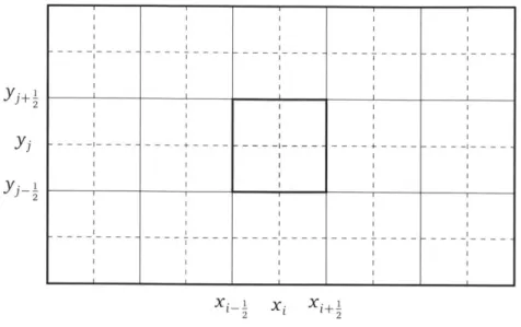
yj+ i yj yj-i 2 I I I I I i I I I I I I I I I I I I I I I I I I I I I I I I I I I I I I I I I I I I I I I I I I I I I I I I I I I - + - +. -I I I I I I I I I I I I I I I I I I I I I I I I I I I I I I I I I I I I I I I I I I I I I I I I I I I I I I I I I X~i X X~~1 2 L 2

Figure 2-1: Discrete ordinates discretization in 2-D Cartesian coordinates. The shaded region denotes cell (ij).

where the emission density q contains all scattering, fission, and external sources. To consider this in more detail, we assume a 2-D Cartesian coordinate system. This pro-vides a slightly more complete set of details than would 1-D without the verbiage of

3-D. In 2-D Cartesian coordinates, Eq. 2.3 becomes

p + r + E, (x, y)%(x, y, p, rj) = q(x, y, p, rj), (2.4) where p and r, are the directional cosines with respect to the x and y axes, respectively. In the discrete ordinates method, a discrete set of angles Q,, n = 1 ... N is selected,

resulting in

±+a , + E(x,y)4a(x,y) = q(x, y), (2.5)

a x a y

where, for example, %n(x, y) = (X, y, EE)

Numerous advanced schemes have been developed for discretizing the SN equations in space; the reader is encouraged to see the rather thorough review of Larsen and Morel [38]. However, to incorporate that body of work is beyond the present scope. Rather, we use a simple finite volume approach. The geometry is discretized in x and

(30)

In each region, the material and source are assumed to be constant. Integrating Eq.

2.5 over the rectangular element [xi, xi+11 x

[yj-1, yj+

] yields

Ailbii~n- b-J~)+ in(bj+, - !n+ Aij-ijbj =zizjqi ₁, (2.6)

where Aj = xiI ₂- Xi,1, ₂ A y _i ₂ - y ₂,

2 2

j X dx

j

dy4n(x,y) (2.7)

2 2

and, for example,

1 +

=

J~

dY'tkn(Xi!, Y). (2.8)

To close the equations, the cell center flux must be related to the cell edge fluxes. The simplest scheme is to define the cell center flux as the average of each pair of opposing edge fluxes,

1 1

which is the well-known "diamond difference" scheme [40]. Assuming neutron travel into the first octant (p, iq > 0), we have

2W, [-,,l _A _,-b _f

(2.10)

V-u±!,n

= 2bijn - b!,n

bij+!,

=

2 bjn -

ki,j-!,

with similar relations for the remaining octants. The last two relations describe a sweeping action, taking known fluxes from a left or bottom boundary and propagating the information across the cell in the direction of travel. Extensions to 1-D and 3-D are straightforward.

(31)

The only unspecified term is the emission density. Because a discrete set of angles has been selected, the integrals of the continuous emission density

E, (X, y)+}1E (x, y)

q(x, y, Q) = ) %b (x, y, Q)dQ + s(x, y, y, q) (2.11)

41Ta

become weighted sums, so that

E (x,y)+ Ef(x,y) N

, wn(xnixy)+sn(x,y). (2.12)

Selecting the quadrature points and weights is a nontrivial task. For 1-D problems, the Gauss-Legendre quadrature is by far the most common, since it can accurately in-tegrate the Legendre moments necessary for anisotropic scattering with comparatively few points. In 2-D and 3-D, the choice is less clear. The level symmetric quadrature has been popular, since it can integrate relevant spherical harmonic moments (needed for anisotropic scattering in higher dimensions). However, other quadratures may be better suited for a particular task, and as discussed in Chapter 5, quite specialized quadratures may be needed for optimal use within the response matrix method.

2.1.2 Method of Characteristics

The method of characteristics (MOC) is an alternative scheme for discretizing Eq. 2.1. The basic idea of MOC is to integrate the transport equation along a characteristic path of neutron travel from one global boundary to another. The obvious benefit of such an approach is that arbitrary geometries can be easily handled. Only MOC as applied to

2-D geometries is considered in this work.

The Characteristic Form of the Transport Equation

Consider again Eq. 2.3. The streaming term n - V4 is just the rate of change of

4'

along the direction of travel, i.e. along the characteristic. This is particularly clear in Cartesian coordinates. Letting r = r' + s, where s is the distance traveled from an

(32)

initial point jO, we have

d dx O dy L dz 0

ds ds 3x ds Oy dsOz

= a + q a + a(2.13)

OX Oy Oz

We can therefore cast Eq. 2.3 in the form

d

--(o+sh, 6) + EY +sh) = q(?0 +sh2, h), (2.14)

which is the characteristic form of the transport equation.

To solve Eq. 2.14 numerically via MOC, the simplest approach is to divide the domain into flat source regions (FSR) in which materials, the scalar flux, and the source are all assumed constant. Tracks are defined across the geometry, from one exterior point to another. Tracks are comprised of segments, portions of the track that exist within a single flat source region.

Equation 2.14 can then be integrated directly along each track segment, beginning with a global boundary and propagating outgoing angular fluxes of one segment to the next. For a single segment of length L and incident flux of %-, integrating Eq. 2.14 exactly yields an outgoing flux

+ =-eL + q (I - eEL) . (2.15)

and average flux

%b - (~1 -etL+ E2 (E (2.16)

EtL E L

This is the so-called "step characteristic" method, which can also readily be applied to the 1-D SN method. As for the SN method, higher order discretization schemes have been developed for MOC (see e.g. Refs. [19] and [39]), but for the purposes of this work, the step characteristic scheme is sufficient.

(33)

The average scalar fluxes /i in the ith FSR are weighted sums of the average seg-ment angular fluxes s, or

Vizi=ZW lW mZ' sLss. (2.17)

1 M sEi

where 1 indexes polar angle, m the azimuth, and s a segment, and where L, is the segment length, 5s is the segment width (possibly constant for m), and Vi is the volume of region i. The emission density is defined in terms of these average FSR fluxes.

Again, similar to the SN method, an angular quadrature is required to define the azimuthal distribution tracks and the polar angles over which Eq. 2.14 is integrated. For the polar dependence, a segment length L represents the length of the segment in the xy-plane, L,Y, divided by the sine of the angle with respect to the polar (z) axis,

or L = LX,/ sin 0.

MOC Tracking

Probably the most common tracking procedure is to employ evenly-distributed az-imuthal angles with a polar angle quadrature based on accurate integration of the Bickley-Naylor functions together with evenly-spaced tracks of some fixed spacing. Frequently, cyclic tracking is enforced, meaning that each track ends exactly where its reflection begins [37]. This perturbs the azimuthal spacing somewhat, but for large enough numbers of tracks, the difference is small.

For this work, a different approach is taken. Any azimuthal and polar quadratures can be used. For each azimuth, tracks are defined with starting points based on Gauss-Legendre quadrature. This allows for highly accurate integration of boundary fluxes over space, a desirable feature for response generation.

Typically, track spacing is an input parameter. Use of uneven spacing complicates this somewhat. Rather, suppose we limit the track spacing to some maximum value,

6

max, and distribute an odd number, n, of Gauss-Legendre points be distributed over the

(34)

Figure 2-2: MOC tracking of a 2-D Cartesian mesh using Gauss-Legendre points. there is an analytic form for wmax as a function of n, a simple rational approximation is

1.585

Wmax R n + 0.5851. _(2.18)

Setting this equal to the allowable spacing and rounding up to the nearest integer gives

1.585

n

[ 1

0.5851 . _(2.19)

Note, only the horizontal or vertical boundary can have a single set of Gauss-Legendre points. For the remaining surfaces, two sets of points are generated due to overlap. However, this still maintains accurate piece-wise integration over the entire boundary. Figure 2-2 shows an example tracking for one quadrant, singling out a FSR of interest to highlight several quantities. Due to symmetry, only the first two quadrants need to be tracked in practice.

Because the end point of one track generally does not coincide with the origin of another track in the reflected direction, reflecting boundary conditions require interpo-lation. However, for response generation, this is not an issue.

(35)

---MOC Geometry

Because MOC discretization is based on following tracks across the domain, the geome-try is not constrained to a mesh of any type. One of the most flexible ways to represent arbitrary models is through use of constructive solid geometry (CSG).

The basic approach of CSG is to combine so-called primitives using the union, in-tersection, and difference operators. Primitives typically include basic volumes such as cuboids or ellipsoids. However, these primitives can actually be further divided into primitive surfaces. In this work, all CSG models are based on this latter approach.

2.1.3 Diffusion Approximation

As an alternative to a full treatment of the transport equation, we can use the simpler diffusion approximation. We present a diffusion discretization here for two reasons. First, the diffusion approximation is central to the preconditioners developed below for accelerating transport solves. Second, several well-known diffusion benchmarks that provide further tests of the response matrix method.

If we take the angular flux of Eq. 2.1 to be at most linearly anisotropic, we arrive at the multigroup diffusion equation

G

-VDg(iDV4Pg(i?) + Erg(Db4g(') =

z

,(

Xg G)g'=1,g'$g (2.20)

+ X

kr,)iZc=)g,

v ?)+Sg(r ), g=1...G

.

kg'=1

Similar to the our approach for the SN equations, we discretize the diffusion equation using a mesh-centered finite volume approach, assuming that cell materials and sources are constant [27]. Consider the one group diffusion equation

(36)

Integrating Eq. 2.21 over the volume Vik, one obtains Zk+1/2 dy fk12dz - VD(r-)V (r-) + E,.(x, Y, _Z)#(X, y, Z) Zk+1/2 z k-1/2 Xi+1/2 d fYj+1/2 dx

_

X_-_/ fj-1/2 (2.22) dzQ(x,y,z), -Diik A A ( 0x i+1_{1 2})

±Ax AZk (kY(YI+1/ ₂)

+Ax AyQ (z k+1/2)

-- _(x _i-112)

- k(Y-1/2))

- &(Zk-1/2))}

(2.23)

+ A A! Azk rijkPijk 4 Axi Ayj AzkQ ijz

where the cell-centered flux and source are defined as 1 1 1 Xi+1/2

#ijk A A A,

Axi y YjAZk _X_i-1/2

Yj+1/2 dx Yj+i/2 Yj-1/2 Zk+1/2 zk-1/2 dz 4)(x,y,z), (2.24)

the cell emission density is

1 1 1 i+1/2

Qijk =

---Axi AYj AZk xi-112

yj+1/2

dx

f

yj-1/2

Zk+1/2

dy dz Q(x, y,z), (2.25)

and, for example, 4x(xi+112) is the derivative of 4 with respect to x, averaged over y and z, and evaluated at x =

xi+12-To evaluate the partial derivatives Ox, #b, and Oz in Eq. 2.23, we employ Taylor expansions. For the x-directed terms, we have

Ax _1

(xi_1,yj,zk) ( 4 (xi-1/2,yj,z k) 2

#x

(xi-1/2,j,zk) (P Xi,Yj, Zk) N (Xi-112, yj, Zk + x x(xi_112,yj, k)

(2.26) ' +1/2 fxi-1/2 fj+1/2 dx Yj-12 or =

(37)

$(Xi+1, Yj, Zk) N (Xi+1/2, Yj,Zk) - x(Xi-112,Yj, Zk)

Ax. X1

0) (Xi~, yj, Z) 4(PXi+1/2,Yj, Zk) + 2L+ (X/21 j k

and similarly for the y- and z-directed terms. By continuity of net current, we must have

(2.27)

Dj_,jkPx(Xi-1/ ₂ yj, Zk) = DiIjz4(Xi+1/2,3j, Zk). (2.28) Multiplying Eqs. 2.26 by Di_1j/Axi_1 and Dijk/Axi respectively yields

Djk(Xi1, j,Zk) Axi1 ) Dik )(Xi,Yj, _Zk) Axj D_1,jk _DjI,jk

= 0 (Xi- ₁/₂,Yj, Zk) 2 x(Xi-112, Yj, Zk)

_D~J Dik

- 0 (Xi-1/2,YjZk) +

)

x(Xi-12, j, _k

Axi 2

and adding the resulting equations and rearranging yields

Oi-1/2,jk

-DjI i_1,jk Ax, + Dijk4)₁jkAXi_₁

D-IJkAx + DjkAXi_1

Substituting this into the second of Eqs. 2.26 gives

Ox(Xi-1/2,YjZk) =

2

Axi ( Oijk

D_1,jIk_1,jkAx₁ + DijkOIjk AXi

D _1,jk A +DijkAXi_1

2 Di, jk)ijkAj + Dijk4)i.,kAXi_1 Axi ( D_₁,)kAx, +

DijkAXi-(Px(Xi-1/2,YjZk) = 2Di_1,jk

Oijk - Oi-1jk

(x

i-jk + Axi_₁Dijk

and similarly

Ox(Xi+1/2, Yj,Zk) = 2Di+1,jk

4 )

i±1,jk - (Pijk

C

AxDi+l,jk + Axi+1Dijk

These equations and the equivalents for y and z go back into Eq. 2.23 to obtain a set

of internal equations. (2.29) (2.30) or (2.31) (2.32) (2.33)

(38)

Substituting the Eqs. 2.32 and 2.33 into Eq. 2.23 yields

Az

[

2Di+1 jk O+1,j - Oi,

2 + x( D i+1,jk + Axi+1Di jk

2D ij',jkj

i- -1,jk + AXi-,Dijk _

(2.34)

Ax Ay AZk Er,ijk/ijk = A yjAj AzkQijk,

G G

Qij f,ij

g'=1 g'=1

g'$g

(2.35)

and where g is the group index that has been suppressed in our development thus far. Equation 2.34 represents the balance of neutrons in the cell (i, j, k).

We can further simplify the notation. Let us define a coupling coefficient 2Di+1,jkDijk

AxiDi+ljk ₊_A _Dijk (2.36)

with similar coefficients for each direction. Then we can rewrite Eq. 2.34 as

i+1,j,k + Di+1/2,j,k (Oj ijk + bi,j+1/2,k (ctijk kYj Sbi,j,k+12

Qi'ijk

Zk - 4Pi,j+1,k + Di 1 2,k (Pijk y j +Di, ,k-1/2 (Pj - 4i,j,k+1) + D k Zk + Zrijk~/ijk = Qijk

-Note that each term on the left with a coupling coefficient represents the net leakage from a surface divided by the area of that surface.

Internal Equation -Dijk

{

_Aj where - i,j-1,k ~ i,j,k-1 (2.37) Di+1/2,jk ( ijk ~ q#i-l,j,k)

(39)

Boundary Equations

At the boundaries, we employ the albedo condition [27]

1 1 1 - 3(x, y, z)

--D(x, y,z)Vo(x, y,z) - (x, y, z)+ - 4x, y,z) =J(x,y,z), (2.38)

2 4 1 + (x, y, z)

where ft is the outward normal, P describes the albedo condition (P = 0 for vacuum or

incident current, and P = 1 for reflection). Additionally, we explicitly include a possible

incident partial current J-, for which P = 0. For reference, the outgoing partial current

is simply

1 11- [(x,y,z)

J+(x,y,z) = -- D(x, y, z)V(x, y, z) -f(x, y, z) + q(x, y, z), (2.39)

2 4 1 + P(x, y, z)

In general, we have six global surfaces, though there can be more depending on whether jagged edges are modeled. However, at a cell level, there are six faces, some of which may be part of a global surface. As an example, we consider the west global boundary:

1 11-/3

west boundary: 2DJkX(x/2,yj,zk) + j st . (2.40)

2

lkO(X1,Y,)4

1 +

1/ ,k i

Because this expression contains q at the edge, we again need to employ Taylor expan-sions. For the west boundary, note that

#ljk #1/2,jk " + x (X1/2, Yj, zk), (2.41)

and we rearrange to get

4

(40)

Placing this into the albedo condition yields

jk 2 Djk1x(xl/2,yj,zk)

Solving for OX(X1/2, Yj, Zk) gives

Ox(X1/2,Yj,Zk) =

2

rx(X112,fj,Zk)

2(1 - #)#ijk - 8(1 + #)Jwest

-4(1 + P)Dlik + Axj(1 - /)

For the east, we similarly find

4

x(XI+1/2,yj,Zk) =

-and likewise for the other surfaces.

2(1 - 3))Ijk - 8(1 +

f)Jast-4(1 + ()Djk + Ax,(1 - P3)

Each of these is placed into the proper partial derivative of Eq. 2.23. For example, the leakage contribution on the left hand side of

Eq. 2.37 due to leakage from the west boundary is transformed as follows1:

D _{/2,jk (} k A 1 - (1)k ) 2 Dljk(l - [) 4 )ljk (4(1 + /)Dljk _{+ Ax,(1 -} _#))AX 1 (2.46)

Notice that the jeast- term is not present; rather, we shift that to the right hand side

as an external source because that term is not a coefficient for any value of the flux. Hence, that source term becomes

boundary Qljk 8_Dljk(l₊_f)J7'est -(4(1 + 1 1 + Ax1(I - x)D (2.47)

Constructing the Diffusion Matrix

The equations for cell balance derived heretofore can be combined into a linear system for the cell fluxes. Generically, we can express this system as

(2.48)

(2.43)

(2.44)

(2.45)

'Ignore the fact that <POik doesn't exist!

L = Q ,

Advanced response matrix methods for full core analysis

Advanced Response Matrix Methods for Full Core

ARCH4VEZ

Analysis

by

APR

08

201k

Jeremy Alyn Roberts

LIBRARIES

B.S./M.S. University of Wisconsin

-

Madison (2009)

Submitted to the Department of Nuclear Science and Engineering

in partial fulfillment of the requirements for the degree of

Doctor of Philosophy in Nuclear Science and Engineering

at the

MASSACHUSETTS INSTITUTE OF TECHNOLOGY

February 2014

Massachusetts Institute of Technology 2014. All rights reserved.

Author ...

Department of Nucl

r

fence andEngineering

eptember 23, 2013

C ertified by ...

...

Benoit Forget

Associate ProfessorLf Nuclear Science and Engineering

Thesis Supervisor

Certified by ...

...

Kord Smith

KEPCO Professor of the Practice of Nuclear Science and Engineering

Thesis Reader

Accepted by ...

...

Mujid Kazimi

Advanced Response Matrix Methods for Full Core Analysis

by

Jeremy Alyn Roberts

Abstract

Acknowledgments

Contents

List of Figures

4'

List of Tables

Chapter 1

Introduction and Background

1.1

The Eigenvalue Response Matrix Method

1.1.1

Neutron Balance in a Node

I

Kl

IL

--

Jil

I

1.1.2 Global Neutron Balance

1.2

Survey of ERMM Methods

1.2.1

Diffusion-based Methods

1.2.2 Transport-based Methods

4

1.3 Major Challenge

1.4 Goals

1.4.1

Deterministic Transport Algorithms

1.4.4 Parallel Solution of the Eigenvalue Response Matrix Equation

Chapter 2

Transport Methods

-

Discretizations

and Solvers

2.1

The Neutron Transport Equation

f2

V'lkg(K