Advanced nonintrusive load monitoring system

Advanced Nonintrusive Load Monitoring

System

by

AWR

1072

Warit Wichakool

S.B. Massachusetts Institute of Technology (2001)

M.Eng. Massachusetts Institute of Technology (2001)

Submitted to the Department of Electrical Engineering and Computer

Science

in partial fulfillment of the requirements for the degree of

Doctor of Philosophy

at the

MASSACHUSETTS INSTITUTE OF TECHNOLOGY

February 2011

@

Massachusetts Institute of Technology, MMXI. All rights reserved.

AuthorA

Department of Electrical isngineering and

Certified by Pro Accepted by Computer Science January 5, 2011 Steven B. Leeb fessor of Electrical Engineering and Computer Science

7 Thesis Supervisor

/

V

Terry P. Orlando Chairman. Departmental Committee on Graduate Theses

Acknowledgments

I would like to acknowledge many individuals and organizations for their valuable assistance throughout the course of this thesis work. Without them, this work would not have been successful.

First of all, I would like to thank Professor Steven Leeb, my advisor, for his guidance throughout my study. Professor Leeb has been one of the greatest mentor I have ever met. His advises have improve myself professionally and personally.

Next, I would like to thank my thesis committee: Professor Leslie K. Norford, Professor James L. Kirtley, and Professor David J. Perreault for their recommenda-tions and suggesrecommenda-tions regarding the thesis work. Their quesrecommenda-tions and comments have make the thesis more completed.

In addition. I would like to extend my acknowledgments to many LEES friends and colleagues. I would like to thank Robert Cox. Al-Thaddeus Avestruz. Jim Paris, Christopher Laughman, John Cooley, Zachery Remscrim, Chris Schantz, Amy Engle-hart, and Uzoma Orji for their contributions to my works. Also, I would like to thank them for many great times in LEES. Also. I would like to thank David Otten, Bran-don Pierquet, Robert Pilawa. William Richoux, Anthony Sagneri. George Hwang, Benjamin Cannon, Jackie Hu. Jiankang Wang, Makiko Wada, Vivian Mizuno, and many LEE for making LEES a great place to work and live throughout my stay at MIT.

Furthermore. I would like to thanks many friends: Nunpon Insin. Clhakra-pan Tuakta, Jin Suntivich, Pin Anupongongarch, Wisuwat Songnuan, Petch Jear-anaisilawong, Pivatida Hoisungwan, Arance Techawiboonwong, Sirimas Sudsakorn. Sappinandana Akamphon, Yotsawan Chaturapornkul, Nisanart Chalearnlarp. Wang Nuitragool. Lalita Chanwongpaisarn, Yui Sanchatjate, Patcharee Srisawasdi, Sira Sri-sawasdi, Soniponnat Sampattavanich, Siwanon Jirawatnotai, and many others for being great friends throughout the great time I have spent throughout the U.S.

Advanced Nonintrusive Load Monitoring System

by

Warit Wichakool

Submitted to the Department of Electrical Engineering and Computer Science on January 5, 2011, in partial fulfillment of the

requirements for the degree of Doctor of Philosophy

Abstract

There is a need for flexible, inexpensive metering technologies that can be deployed in many different monitoring scenarios. Individual loads may be expected to compute information about their power consumption. Utility providers, facilities managers, and other consumers will likely find innumerable ways to mine information if made available in a useful form. However, appropriate sensing and information delivery systems remain a chlief bottleneck for many applications, and metering hardware and access to metered information will likely limit the implementation of new electric energy conservation strategies in the near future.

This thesis presents solutions for two long standing problems in nonintrusive power and diagnostic monitoring. First, a high-resolution, physically windowed sensor architecture that is well-suited for energy score-keeping and diagnostic applications will be discussed. The sensor can track a large-scale main signal while capturing small-scale variations. The prototype system uses digital techniques to reconstruct an observed current with a high effective bit resolution. The sensor measures a small current signal using a closed-loop Hall sensor. and extends the range by driving a compensation current with a high performance current source through an auxiliary winding. The system combines the compensation command and the sampled output of the residual sensor to reconstruct the input signal with high bit resolution and bandwidth.

Second, a long-standing problem in nonintrusive power monitoring involves the tracking of power consumption in the in the presence of loads with a continuously variable power demand. Two new techniques have been developed for automatically disaggregating, in real-time. different classes of continuously variable power electronic loads which draw distorted line currents. Experimental results of the proposed power estimator extracting the power consumption of common variable power loads such as a variable speed drive, a computer, and a light diummer are presented.

Thesis Supervisor: Steven B. Leeb

Title: Professor of Electrical Engineering and Computer Science

I am also greatly

thankful

for my family for their encouragement and support

through all my life.

Finally. I would like to thank many sponsors including Thai Government for

the financial support and more importantly the opportunity to pursue the study at

M.I.T.

Contents

1 Introduction

13

1.1

Nonintrusive load Monitoring . . . .

14

1.2 Scalability . . . .

23

1.3

Challenges . . . .

24

1.4 Thesis Organization... . . . .

. . . . .

25

2 Physically-Windowed Sensor

28

2.1 Introduction . . . .

28

2.2 System Design . . . .

29

2.2.1

Current Measurement

. . . .

29

2.2.2

System Architecture

. . . .

32

2.2.3

Signal Reconstruction

. . . .

34

2.2.4

Resolution and Range . . . .

36

2.2.5

W indowing . . . .

37

2.2.6

Bandwidth . . . .

38

2.3 Benefits and Motivation . . . .

39

2.3.1

Resolution . . . .

40

2.3.2

Bandwidth . . . .

40

2.4 Prototype Implementation . . . .

42

2.4.1

Closed-Loop Hall Sensor . . . .

43

2.4.2

Clamp Circuit . . . .

45

2.4.3

Residual Current Measurement . . . .

45

2.4.4

Compensation Current . . . .

47

2.4.5

Microcontroller . . . .

49

2.4.5.1

Sampling . . . .

49

2.4.5.2

W indowing Strategy . . . .

51

2.4.5.3

Communication . . . .

52

2.4.5.4

Calibration . . . .

52

2.5

Prototype Results . . . .

53

2.5.1

Full system functionality . . . .

53

2.5.3 Dynamic resolution tests... . . . . . . . .. 57

2.5.4 Residual sensor transient response... ... .. . . . .. 57

2.6 Summary. . ... . . . . . . . .. 60

3 Variable Speed Drive Power Estimator

61

3.1 Introduction . . . .

61

3.2 B ackground . . . .

63

3.3 V SD M odel . . . .

68

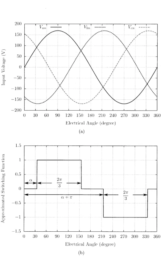
3.4 Switching Function . . . .

71

3.5 Estimator Derivation . . . . 75

3.5.1 Switching Function Approximation . . . . 75

3.5.1.1 Ideal Switching Function . . . . 76

3.5.1.2 Approximated Switching Function . . . . 78

3.5.2 Dc-side Harmonies Approximation . . . . 80

3.5.3 Estimator Coefficients . . . . 87

3.6 Results and Discussion . . . . 88

3.6.1 Balanced Input Voltage Cases . . . . 89

3.6.2 Distorted input voltage cases . . . . 89

3.7 Sum m ary . . . . 95

4 Waveform-Based Estimator

96

4.1 Introduction . . . . 96 4.2 Background . . . . 98 4.3 Waveform-Based Estimator . . . . 107 4.4 Estimator Derivation . . . . 109 4.4.1 Signal Constraints . . . . 110 4.4.2 Matrix Equation . . . . 116

4.4.3 Reduced Row Echelon Form . . . . 117

4.4.4 Estimator Evaluation . . . . 118

4.4.5 Numerical Instability . . . . 121

4.5 Cyclotomic Field Representation . . . . 123

4.5.1 Roots of Unity . . . . 123

4.6 Experimental Results . . . . 126

4.6.1 Variable Speed Drive . . . . 127

4.6.2 Com puter . . . . .. . . . . 130

4.6.3 Light Dimmer . . . . 132

4.7 Sum m ary . . . . 136

5 Conclusion and Future Work

140

7-A Circuit Schematic for Physically-Windowed Sensor

145

B Computations of weighting coefficients for the VSD estimator

158

List of Figures

1.1 1.2 1.3 1.4 1.5 1.6 1.7 1.8

Coast Guard Cutter USCGC Escanaba . . . . Simplified block diagram of a NILM system . . . . . NILM sensing hardware . . . . Current sensor installation . . . . Turn-on transient of an induction motor . . . . Turn-on transient of an incandescent lamp . . . . Power consumed by the three-phase induction motor Real power consumed by the incandescent light bulb

. . . . 16 . . . . 17 . . . . 18 . . . . 18 . . . . 19 . . . . 19 . . . . 21 . . . . 21

2.1 Examples of isolated current sensors . . . . 30

2.2 System block diagram of the physically-windowed sensor . . . . 32

2.3 Example of a signal reconstruction for the physically-windowed sensor 33 2.4 Detailed block diagram of the prototype system. . . . . 34

2.5 Overlap of the DAC output, relating to compensation current, and the ADC input. relating to the residual measurement... . . . .. 36

2.6 Detailed block diagram of the prototype system... . . . . . . . 43

2.7 Full system block diagram... . . . . . . . .. 43

2.8 Circuit diagram of the customized closed-loop Hall sensor and the ac-tive clamp... . . . . . . . .. 44

2.9 System block diagram of the closed-loop Hall sensor . . . . 44

2.10 Calibration curves showing 11-bit residual current measurement versus 10-bit compensation current command, at various fixed primary currents 46 2.11 Compensation current driver circuit diagram... . . . . .. 47

2.12 Output stage of the compensation current subsystem. showing the OTA implementation... . . . . .. 48

2.13 Prototype implementation... . . . . . . . . 50

2.14 Windowing approach in the prototype implementation . . . . 51

2.15 Oscilloscope traces showing the measured primary, compensation, and residual measurement currents while the prototype physically win-dowed current sensor is in a normal operation... . . . .. 54

2.16 Reconstructed current from the prototyped sensor... . . . . .. 55

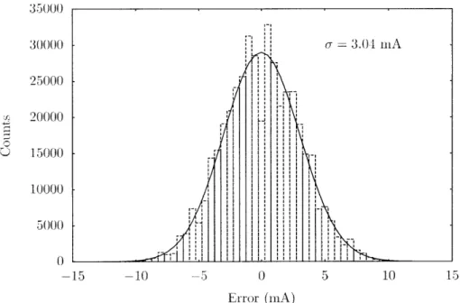
2.17 Histogram of the measured errors during a test of de performance . 56 2.18 Example of measuring a small de current on top of a large ac current 58 2.19 System response during a high current transient . . . . 59 3.1 A snapshot of the line current consumed by an incandescent light bulb

and a VSD over one cycle of the line voltage from the experimental setup 65 3.2 Experiment result showing the power consumption of a VSD, a

three-phase rectifier, and an incandescent light bulb. . . . .. 65 3.3 Experimental result showing the in-phase components of harmonic

cur-rents consumed by the VSD and three-phase rectifier... .. 66 3.4 Experimental data and the correlation function between the in-phase

component of the fundamental and the fifth harmonics used to derive the empirically-based estimator... . . . . . . . . . 67 3.5 Block diagram of the model-based VSD power estimator... . . . . 68 3.6 A simple circuit model of the VSD equipped with an uncontrolled

rectifier used to simulate the VSD current waveforms.. . . . . .. 69 3.7 Reference input voltage and simulated line current consumed by the

three-phase uncontrolled rectifier... . . . . . . .. 70 3.8 Examples of the dc-bus current. the switching function, and the ac-side

current when the input voltages are balanced and the VSD system is operating in a steady state from the simulation... . . . .. 71 3.9 The process of computing the line current harmonic as a modulation

of the dc-bus current by the switching function . . . . 74 3.10 Block diagram showing the process of estimating the VSD fundamental

harmonic current from a set of higher harmonic currents . . . . 76 3.11 Simulation results showing the ideal switching function for phase-A

current and the ideal three-phase voltage when the input voltages are balanced . . . . 77 3.12 Simulation results showing the non-ideal input voltage and

approxi-mated switching function for the phase-A current.. . . . . . . . . 79 3.13 Simulated dc-bus current of the VSD three-phase uncontrolled rectifier 81 3.14 Simulated dc-side harmonic current of the three-phase uncontrolled

3.15 Examples of dc-bus and ac-side current waveforms in a general case. . 85

3.16 Experim ental setup . . . . 88

3.17 Experimental results of the VSD power estimator resolving the power consumption of VSD and rectifier from the 50-W incandescent light bulb under balanced input voltages . . . . 90

3.18 Experimental result showing the estimated power of the 50-W light bulb after the empirically-based estimator has removed power of the VSD and the rectifier under the balanced input voltages . . . . 91

3.19 Experimental results showing the estimation errors in the VSD real power prediction using when the input voltages are distorted with dif-ferent levels of fifth harmonic . . . . 92

3.20 Experimental results showing the estimation errors in the VSD real power prediction using different VSD power estimators when the input voltages are distorted with different levels of seventh harmonic . . . . 93

3.21 Experimental results showing the estimation errors in the VSD real power prediction using the model-based estimator with four input har-m onies . . . . 94

4.1 Simulated current waveforms and normalized harmonic currents of a variable speed drive . . . . 100

4.2 Experimental current waveforms and normalized harmonic currents of a computer. . ... . . . . . .. 101

4.3 Experimental current waveforms and normalized harmonic currents of an incandescent light dimmer. ... . .. 102

4.4 Correlation functions of the harmonic currents of the computer . . . . 103

4.5 Real and reactive power consumed by the light dimmer . . . . 104

4.6 Correlation functions of the harmonic currents of the light dimmer . . 105

4.7 Current waveforms of multiple variable power loads... . . .. 106

4.8 Regions of zero-current of the VSD... . . . .. 111

4.9 Estimator evaluation error plots... . . . . . .. 120

4.10 Floating-point arithmetic errors... . . . . . .. 122

4.11 Complex exponentials roots for N = 12 . . . . 125

4.12 Experimental setup for testing the VSD estimator... . . . . . . 128

4.13 Demonstration the waveform-based estimator extracting the real power consumption of the VSD from the incandescent light . . . . 129

4.14 Regions of zero-current of the computer... . . . . . . 131

4.15 Experimental setup for testing the computer estimator . . . . 132

4.16 Demonstration of the waveform-based estimator extracting the real power consumption of the computer from the incandescent light. . . . 133

4.17 Regions of zero-current of the light dimmer... . . . . . . . . 134

4.18 Experimental setup for testing the light dinner estimator . . . . 136

4.19 Demonstration the waveform-based estimator extracting the real power consumption of the light dimmer from the incandescent light . . . . . 137

4.20 Demonstration the waveform-based estimator extracting the real power consumption of the light dimmer from the incandescent light . . . . . 138

A.1 Schematic of the control power . . . . 146

A.2 Schematic of the unregulated power supply . . . . 147

A.3 Schematic of the power supply for the control circuit . . . . 148

A.4 Schematic of the command voltage . . . . 149

A.5 Schematic of the digital-to-analog converter (DAC)... . . . .. 150

A.6 Schematic of the DAC isolation circuit and the microcontroller power supp ly . . . . 151

A.7 Schematic of the USB peripheral . . . . 152

A.8 Schematic of the microcontroller connection . . . . 153

A.9 Schematic of the 12-bit analog-to-digital converter (ADC) . . . . 154

A.10 Schematic of the 12-bit ADC isolation circuit . . . . 155

A.11 Schematic of the the 24-bit ADC . . . . 156

A.12 Schematic of the 24-bit ADC isolation circuit . . . . 157

C.1

Pseudo-code for the waveform-based estimator.. . . . . . .. 162

-Chapter 1

Introduction

The U.S. government realizes the importance of the electricity sector and its future, the Energy Independent and Security Act of 2007 has been passed to encourage and focus the effort to improve the current electricity grid and distribution system. The Title XIII of this law has identified a list of actions to characterize a "Smart Grid." One of the action items includes a "deployment of -smart' technologies ... for metering, communications concerning grid operations and status, and distribution automation." Another action item includes an "integration of 'smart' appliances and consumer devices." Additionally, the law also calls for a "development and incorporation of demand response, demand-side resources, and energy-efficiency resources"

[I].

The Smart Grid would require "smart" metering devices and communication networks to collect and deliver necessary information about the power system for the operation of the power grid. Given a require communication networks, smart meters can provide the information about the power consumption for utilities and electricity consumers almost instantly. Many smart metering projects can be seen many places in the U.S. and other countries such as England. The real-time information is one of the tools for the dynamic pricing program. where the electricity price could change depending on the time-of-use for example [2,3]. The accessibility of the power con-sumption in real time would allow the consumers to adjust the electricity utilization in order to minimize the electricity bill. In fact, the project report on the smart meter in England has shown that some consumers become more energy efficient users and lower their electrical bills [4].

These smart metering projects have shown that the electrical distribution

work can provide not only the power distribution but also an information provider for power planning and adjustment in real-time. The power consumption is not the only information that a "smart" meter can extract from the electrical voltage and cur-rent signals. Many diagnostic parameters of loads can also be measured and learned from the electrical signals as well. Diagnostic parameters such as the rotor speed of the induction motor and high frequency variation of the power consumption can provide additional information about the health of these loads. These diagnostic pa-rameters require complex sensing hardware and information extracting algorithms to obtain key parameters from the electrical measurements. The need to collect detail information about individual load has led to the development of a nonintrusive load monitoring (NILM) system.

1.1

Nonintrusive load Monitoring

The development of high bandwidth networks has made an old dilemma increas-ingly more apparent: although networking makes it easy and inexpensive to obtain information from remote sensors. useful information can only be gathered by a po-tentially expensive and intrusive sensor array. Although mass production may ulti-imately reduce sensor cost, especially for solid-state or technologically advanced micro-electromechanical sensors, installation and analysis will likely remain expensive. The overall reliability of a monitoring system with many sensors may be reduced in com-parison to a system with relatively fewer sensors. The utility of data collected with a monitoring system is critically dependent on the ability to perform relevant and fast analysis of the collected data. More sensors may provide more potentially useful information, but at increased cost and increased burden in collating and correlating relevant observations.

On combat vessels. niodern propulsion plant monitoring systems, for example, rely on hundreds of sensors installed throughout the main machinery space. Although

these sensor networks enable increased levels of automation, they are costly to install and to maintain. As these networks grow to include more sensors, there is a corre-sponding drop in the in the overall reliability of the monitoring system.

Fortunately, the growing reliance on electrically actuated systems provides a new opportunity to reduce sensor count. The basis for this clam lies in the fact that electrical currents contain significant information about the physical condition of individual loads. A device that monitors aggregate current at a central location can then disaggregate and track the behavior of multiple downstream components.

A nonintrusive load monitor (NILM) is a system that can determine the oper-ating schedule of electrical loads at a target site using centralized measurements [5,6]. In contrast to other systems, the NILM reduces sensor cost by using relatively few senors. The NILM disaggregates and reports the operation of individual electrical loads like lights and motors using only measurements of voltage and aggregate cur-rent at the service entry to an electrical panel.

Over the last decade, the NILM system has been developed and improved as a nearly sensor-less platform for monitoring mission critical electromechanical loads on warships and office buildings [5, 7 191. Field experiments have been conducted on board two US Cost Guard Famous Class Cutters, the USCGC Escanaba and

USCGC Seneca. The Coast Guard Cutter USCGC Escanaba is shown in Figure 1.1.

Additional load monitoring research opportunities have been explored for US Navy ships, including the DDG-51 class destroyer, through experiments conducted at the Navy's land-based engineering site (LBES). Until recently, most of these experiments have focused on particular engineering subsystems [20,21].

In the recent years, new hardware and software have been developed for the NILM. Experimental results have shown the ability of the improved load monitoring system to provide useful information while underway, augmenting the routine obser-vations traditionally made by a maintenance crew. In some cases. the NILM system has provided new information for which no sensor has been previously installed. The

Figure 1.1: Coast Guard Cutter USCGC Escanaba

NILM has been installed to monitor small collections of electrical loads and also initi-ates studies that consider how many electrical loads a NILM can successfully monitor on a shipboard power system. The goal was to develop a practical lower bound on the power changes that can be effectively detected by a NILM installed at the switchboard level.

Power system monitoring is an exciting approach for creating an inexpensive, highly capable "black-box" for monitoring the performance of critical shipboard sys-tems. With remarkably little installation effort and expense, the NILM has been installed that can reliably monitor and track diagnostic conditions for multiple de-vices. The NILM can be used to determine the need for maintenance, to identify fault conditions, to find power quality problems, to help configure a power system after damage, and to provide reliable verification of load operation. Generally, the power distribution system can, with the proper signal processing and data analy-sis. be made to serve "dual-use." Specifically. it can simultaneously be used for its intended function of power delivery and as an information network for monitoring critical loads.

As previously noted, the NILM makes measurements of voltage and current solely at a single point in the electric utility service. The NILM characterizes indi-vidual loads by their unique signatures of power drawn from the utility. A transient detection algorithm can identify when each load turns on and off, even when several

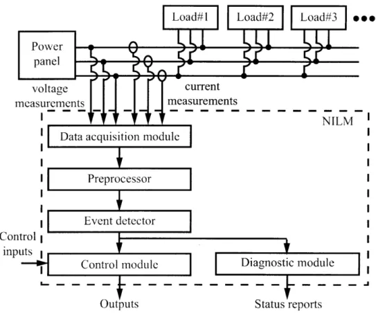
Load#1 Load#2 Load#3 1 e0e Power panel voltage measurements Data acquisi 1 Prepro Event d Control inputs NILM

Outputs Status reports

Figure 1.2: Simplified block diagram of a NILM system

loads do act nearly simultaneously. This monitoring can be performed with relatively little hardware: a computer, an analog-to-digital converter (ADC), and a single set of current and voltage sensors. A simplified block diagram of the NILM is shown in Figure 1.2. The NILM sensing hardware and the sensor installation are shown in Figures 1.3 and 1.4.

When installing a NILM to monitor multiple loads on a ship or other target system, the NILM undergoes a training phase. During training, the NILM observes individual electrical transient events that occur during the operation of particular loads. Examples of transient events that might be observed by a NILM are shown in Figures 1.5 and 1.6. Figure 1.5 shows the turn-on transient of an induction motor. Figure 1.6 shows the turn-on transient of an incandescent light bulb. Each electrical load performs a different physical task, and each load consumes power in a relatively

Figure 1.3: NILM sensing hardware

Figure 1.4: Current sensor installation

-15 10 ... 0 -5 10 --15 0 0.2 0.4 0.6 0.8 1 Time (s)

Figure 1.5: Turn-on transient of an induction motor

30 25 20 - 15- 10-5 15 -20 - 0 0.20.41 0.60. Timie (s)'

Figure 1.6; Turn-on transient of an incandescent lamp

-unique way associated with its task. The three-phase induction motor shown in

Figure 1.5, for example, shows a large pulse of current during the acceleration of the

rotor, and then settles to a smaller steady state current. The incandescent light bulb shown in Figure 1.6 also draws a pulse of current at the turn-on transient, and settles down to a smaller but different steady state current demand. These transients serve as "fingerprints" that can be used to identify the operation of a particular type of load, even when several loads are operating at the same time.

In practice. the NILM examines and recognizes fingerprints by looking for known shapes in "spectral envelopes" or short-time estimates of the envelope of fre-quency content in the current waveform. Examples of the spectral envelopes of the three-phase induction motor are shown in Figure 1.7. An example of the spectral envelope of the incandescent light bulb is shown in 1.8. The NILM examines the spectral envelopes of the line frequency currents both in-phase and quadrature to the line voltage, as well as higher harmonics. The spectral envelope that is computed us-ing the in-phase component of the fundamental frequency current can be referred as the real fundamental power or the real power. On the other hand, The spectral enve-lope that is computed using the quadrature component of the fundamental frequency current can be referred as the reactive fundamental power or the reactive power. The spectral envelope can be computed for higher harmonics such as the third harmonic

as well. 180 Hz on a 60 Hz utility.

In the past. many researches have been conducted to explore the possibility of using a nonintrusive approach to diagnostic monitoring. The NILM has been installed at many sites, including the Coast Guard ships. Several key systems in the Coast Guard ships have been monitored, including auxiliary seawater (ASW) pumps, vacuum-assisted wast disposal system (collection-hold- transfer or CHT), and reverse osmosis (RO) water purification systems. The observations have been done both in-port and underway during operational cruising.

The unique signatures presented by different classes of loads create an

-0.4 0.6 Time (s) (a) 0.1 0.6 0.8 1 Time (s) (b)

Figure 1.7: Power consumed by the three-phase induction motor. The real power consumed by the three-phase induction motor is shown in (a). The reactive power consumed by the three-phase induction motor is shown in (b).

1000 800 600 400 200 0 -200 0.2 0.4 0.6 0.8 Time (s)

Figure 1.8: Real power consumed by the incandescent light bulb

21 -10000 8000 6000 1000 2000 0 10000 8000 6000 4000 2000 0

portunity for diagnostic monitoring. Once it becomes possible to associate observed waveforms or segments with specific loads, it is possible to perform state and pa-rameter estimation non the observed waveforms to track diagnostic papa-rameters for individual loads. For example, the NILM has been used to determine several impor-tant operating parameters of the ASW system. The ASW system provides cooling for all heat loads on board the ship with the exception of those associated with the main diesel engine cooling. Heat loads are cooled by the ASW include the heating ventilation and air-conditioning (HVAC) units, refrigerators, freezers, diesel engine air coolers, and diesel engine lube oil coolers. The ASW system provides an excellent example of the diagnostic capabilities of the NILM. A coupling that connects the ASW pump motor to the pump head can fail leaving the ship temporarily without cooling, which is a major mission complication. Field data collected from the ship has shown that the high frequency "ripple" resents in the spectral envelopes during the transients increased as the coupling progressively failed [11, 22].

To further demonstrate the diagnostic capability of the NILM system, the non-intrusive monitoring system was installed at the entry service of the vacuum-assisted wast disposal system (collection-hold-transfer or CHT) in the USCGC Escanaba. The CHT system represents a common auxiliary system used to transfer sewage through-out the ship to a sanitary collection tank where it is pumped overboard. The operation of the CHT system has been described in [23, 24]. In these diagnostic experiments, the NILM monitored two vacuum pumps that are responsible for maintaining the pressure to operate the sewage collection system. The NILM diagnostic module has detected a possible failure in the system based on excessive cycling of the pumps [24]. An additional research has been done to automate the diagnostic monitoring and load tracking algorithms [15].

Examples in diagnostic monitoring applications shown above have demon-strated the benefit of the NILM system to provide crucial information maintaining effective mission critical system. verifying the health of subsystems, and preventing

any

major

failure by warning of any potential problem. The nonintrusive monitoring concept can be applied in to detect potential problems for a new load in the future as well.

1.2

Scalability

As the NILM has continued to track power consumption and diagnostic parameters

of the loads, the NILM system is naturally expanded to cover more loads. Additional

loads may be added to the power distribution increases the power consumed at the

monitored site. Effectively., the range of measured current increases accordingly. This

increased signal range directly affect the size of measuring sensors. More importantly,

a larger range of measured signals could impact the ability of the NILM to track the

power consumption of individual loads and extract key diagnostic parameters from

the aggregate measurements. A different area of the nonintrusive load monitoring

research is to find the limitation of the sensitivity of the NILM.

In the field, the NILM has been installed to monitor a subset of loads at the

sub-panel of the power system. By monitoring the power panel close to the load,

the NILM can collect information about a particular load without much interference

from other loads, assuming the local sub-panel only services a few loads. A current

transducer (CT) installed at the local sub-panel is usually chosen such that it can

measure the entire range of current delivered by the sub-panel without saturation. If

the sensor becomes saturated, the output signal will be distorted. As a result, many

crucial diagnostic parameters such as transient spectral envelopes derived from the

distorted input waveform could be incorrect. In addition. the diagnostic conclusion

obtained from the output of the saturated sensor would be incorrect.

In the situation where the NILM is installed at a larger power panel that is

located further from the load. In this case. the NILM is expected to monitor a group

of loads that consume more power. Typically, the power panel for these loads is

-located further from the load. Also, the breaker panel is usually rated for higher

current value. As a result. a bigger CT is installed to account for a larger current

range. A bigger CT prevents the measured current signal from saturating the sensor

circuit. At the same time, a larger CT could reduce the measuring resolution of the

signal.

As shown in Figure 1.2, the output of the CT is sampled by the

analog-to-digital converter (ADC) in order to convert the measured current for the analog-to-digital

processing programs in the computer. Given the same electrical load consuming the

same power, the larger CT of the same type will output a smaller signal. Therefore,

the digitized signal will be small as well. One important issue arises as a consequence

of the smaller input signal is a measurement error because of a lower signal-to-noise

ratio (SNR). The error can come from a random noise source or a quantization error.

The impact of the quantization error for the NILM system has been studied in [16].

The study has shown that NILM system can still detect and track certain classes of

loads even though the sensing signal has been scaled down and heavily quantized by

the ADC using an improved matching algorithm [16].

1.3

Challenges

For a given current sensor, the algorithm presented in [16] has improved the NILM

in terms of load recognition for a larger group of load. However, the diagnostic

monitoring applications that rely on a small amplitude signal embedded in a larger

current signal such as a principal slot harmonic (PSH) would suffer from a small

input signal. The PSH can be used to determine the speed of the induction machine.

which can be useful to determine other physical parameters in the system [18., 33].

Specifically, a lower SNR signal has a higher noise floor that might corrupt the PSH

signal causing an error in the speed estimation. When the interested signal is very

small compared to the overall signal. it would be advantageous to have a sensing

module that can extract the detail information from the large signal with a good

resolution and dynamic range.

In addition to the resolution and sensitivity issue of the sensor as the NILM

is expanded to monitor more loads. the NILM is likely to include different classes

of loads. In fact, many electrical loads do not have a fixed power consumption.

The application of power electronics allows the load to operate continuously across

a wide power range. This ability to dynamically adjust the operating point enables

the appliances to perform the task more efficiently and optimally depending on the

program settings. This behavior means that the load would not have a unique power

consumption level nor a unique start-up transient anymore. As a result, the fixed

pattern recognition algorithm would not work with the variable power loads.

Vari-able power loads can been seen in many modern appliances such as variVari-able speed

drives, computers, dimmer, washing machines. dryers, heaters, etc. These loads are

common in many industries and office buildings. The introduction of variable power

loads causes the NILM to adjust the load disaggregation strategy to address the load

disaggregation method.

The sensor resolution and the disaggregation of variable power loads have presented long standing problems for the nonintrusive load monitoring applications. This thesis explores the solution to these two issues and provides feasible solutions both problems. The sensor resolution is addressed by the modification of the current sensor design. On the other hand, the tracking of the variable power loads can be addressed by two different algorithms that can extract the power consumption of the variable power loads from the aggregate measurements.

1.4

Thesis Organization

This thesis addresses two long standing issues that the traditional NILM has en-countered: the sensor sizing and the tracking of variable power loads. The proposed

solutions for this two problems are separated into the sensing hardware and the detec-tion algorithm. In Chapter 2, the thesis describes an alternative way to measure the current waveform that decouples the dynamic range and the resolution in the design process. The ability to separate these two competing parameters allows the design of the sensor to be optimized for a specific application. The chapter explains the design process and trade-offs of design parameters. The sensor prototype has been built and demonstrated in the chapter as well. The proposed prototype has proved the concept of separating the dynamic range and bandwidth for the NILM application.

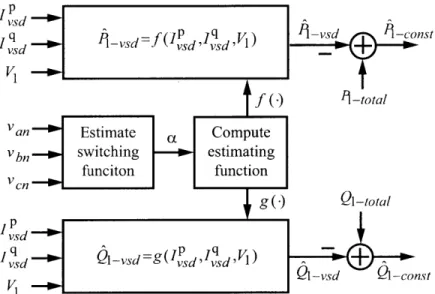
In Chapter 3, the thesis describes the circuit model-based estimator that can track the power consumption of the variable speed drive using higher harmonic cur-rents uniquely associated with the VSD at the monitoring site. The proposed algo-rithm uses a simplified circuit model to study the behavior of the VSD system. From the circuit model, the system approximation is done to the generation of the current signal by thinking of the problem in term of the modulation between the internal current signal and the switching function. The switching function is derived from the behavior of the uncontrolled rectifier in the VSD system. Experimental results are included to demonstrate the ability of the proposed VSD power monitoring algorithm based on the simplified circuit model.

In Chapter 4, the estimator for the variable power loads have been revisited and modified. The second estimator is based on the observation of the current wave-forms of the variable power loads. The structural features of the wavewave-forms can be formulated into a set of linear constraints based on the Fourier analysis and synthesis equations. By applying a linear algebra method such as the Gaussian elimination, the estimator coefficients can be computed. The waveform-based estimator general-izes the process to derive the estimator for any load that consumes non-sinusoidal current waveform. The most useful benefit. is that the algorithm does not need to know about the internal circuit construction of the load. Only the behavior of the current is required in order to compute the coefficients. In this case, the process is an

iterative method. Experimental results show the power tracking of VSDs, computers,. and TRIAC-based light dinnner.

These three proposed solutions enable the NILM system to continue to use the patter recognition algorithm for the fixed power loads and use the proposed power estimator algorithms for the variable power loads. The proposed current sensor also allows the NILM to collect detailed information of the small load in the aggregate stream by using the physically-windowed sensor. The improved NILM can provide the necessary information for the demand side management program and other load diagnostic applications. The proposed solutions could potentially be integrated in the future "smart" metering device can provide information other than an overall power consumption of the consumer.

-Chapter 2

Physically- Windowed Sensor

2.1

Introduction

In energy score-keeping and diagnostic applications, current sensors are often de-ployed to collect and analyze current waveforms from a collection of loads [5]. Anal-ysis provides load disaggregation and detection, power consumption profiling, and diagnostics based on electrical signatures [5, 8. 10,11,13]. Many current sensors are available according to dynamic range and sensitivity. Hall sensors, flux-gate sensors. and Rogowski coils have all been used for non-contact current measurement

[25-31].

As monitoring systems grow to include more loads and to provide more detailed in-formation about the loads, the scalability and utility of the system depends on the quality of data acquired by the current sensor [16]. When monitoring large loads or collections of loads, some relevant features may be found in harmonics or aperiodic contents that are small compared to the current drawn at the fundamental line fre-quency. For other features, the full amplitude signal may be required. In order to collect both small details and overall picture of the signal of interests, the sensing unit should have a wide dynamic range to follow the overall behavior of the signal and good sensitivity to resolve fine features in the signal. These requirements could present opposing specifications for the sensor front-end.

For example, in an electrical system, an induction motor draws the current whose main component is at 60 Hz. On the other hand, a small signal such a principal slot harmonic (PSH) of the induction machine is embedded in the current signal at higher frequency [18]. In this situation, it is advantageous to have a single sensor that

can capture both the power and the PSH of the induction machine altogether. To offer a flexible trade-off between bandwidth and dynamic range, a physically windowing sensor architecture is introduced. Large-scale variations are canceled so that the measured signal remains within a small operating window, which can be measured with a very accurate sensor. This architecture is similar to that of pipelined analog-to-digital converters [32]. but utilizes a physical cancellation approach that can be applied to magnetic flux-based current sensors, strain gauges, pressure transducers, and many other physical systems. The cancellation is controlled by an embedded microcontroller. permitting a variety of windowing techniques and flexible processing and analysis. This thesis presents an initial application of this concept to power electronics and power system monitoring by developing a physically-windowed sensor for a current measurement that demonstrates high accuracy over a wide input range.

2.2

System Design

2.2.1

Current Measurement

In NILM applications, the NILM system extracts power consumption information and device parameters from the collected current measurements through digital sig-nal processing (DSP) techniques. The underlying voltage and current measurements are converted into a digital format through an analog-to-digital converter (ADC) unit. The sensing system must provide a method to convert the current into a digital form that can be promptly used by the DSP unit. Practically, the ADC unit can be care-fully chosen to have enough bits and bandwidth to satisfy the system requirements.

A simple way to measure the current is to pass the current through a shunt resister and measure the voltage across the resistor according to Ohm's law,

'ncas = zactuaiR.

(2.1)

-Vhall

+

Vhall

Vmeas

(a) Open-loop (b) Closed-loop Figure 2.1: Examples of isolated current sensors

The voltage is proportional to the current assuming the resistor value remain unl-changed. The measuring resistor that can stay stable for the required resolution is also available. A high value resistor provides a large output signal but also dissipates more power from the system. On the other hand. a small value resistor does not dis-sipate much power. However, the sensed voltage is small. The choice will be system dependent, and requires additional circuitry for galvanic isolation.

An isolated current measurement technique can employ a magnetically cou-pling system to infer the measured current by measuring the magnetic field strength

H along the closed path C produced by the enclosed current ienciosed according to

Ampere's law,

J

Hdl

=

ienciosed

(2.2)

JC

Examples of isolated current sensing systems are shown in Figure 2.1. The isolated sensing method provides a galvanic isolation between the input circuit and the sensing system. This sensing system usually consists of a flux concentration core and a flux measuring element. The flux measuring device such as a Hall element that give the

output voltage, Vhall, _{proportional to the magnetic flux density}

_B,

Vhall OC B = kiaB. (2.3)

In turn. the magnetic flux density B is proportional to the the magnetic field strength

H in by a permeability p,

B = pH.

(2.4)

The sensing system can measure this voltage directly to infer about the input cur-rent. This system is an open-loop Hall sensor as shown in Figure 2.1a. The system performance depends largely on the Hall element in both resolution and range. A variety of Hall sensors and core structures can be used. Accuracy and precision will depend both on the Hall effect sensor and also the magnetic core. which may have significant nonlinearity.

The sensor performance can be enhanced by using a closed-loop Hall sensing system as shown in Figure 2.1b. In this case, the system uses the output voltage of the Hall element to drive a nulling current intil to keep the flux in the air-gap near zero. The nulling current in₁₁n is then measured through a ballast resistor. This nulling current

inun

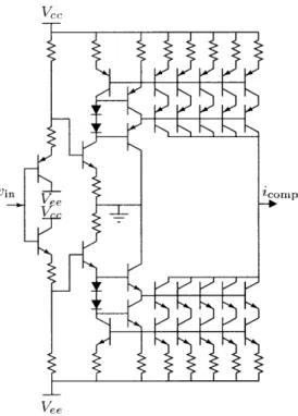
is proportional to the actual current by a turns ratio. In this case, the use of the feedback with a high gain operational amplifier (OpAmp) can reduce the measurement error by the inverse proportion of the open-loop gain of the system. The small signal bandwidth of the sensor is also extended by the feedback loop. The closed-loop senor can provide a favorable bandwidth and accuracy trade-offs for a sensing system. The chosen sensing system must provide adequate dynamic range and resolution.

-icomp

Compensation'

VDAC

Current

,_Driver.

Figure 2.2: System block diagram of the physically-windowed sensor. The system consists of three primary components: the compensation current driver, the resid-ual current measurement, and the microcontroller logic. The compensation current icomp is subtracted from the primary input current factuai by physical cancellation of magnetic flux.

2.2.2

System Architecture

In contrast to a traditional method that uses a single sensor and an analog-to-digital converter (ADC) combination to measure the signal, the proposed architecture aims to achieve both wide dynamic range and high resolution by dividing up the measuring range into smaller pieces. This smaller range can be measured with a reasonable resolution sensor, while the whole system keeps shifting a measuring window up and down according to the input current. This concept can be shown for the current measurement in Figure 2.2.

The windowed sensor architecture resolves the signal as a compensation offset and a measured detail signal. The system must reassemble the actual signal to faith-fully represent the input

measurement.

Figure 2.3 depicts the signal reconstruction

used to determine the total current using the windowed measurement.

Like the closed-loop Hall sensor. the proposed architecture uses physical input

to apply a calibrated cancellation signal to the front-end sensor. In the windowed

approach, two cancellation signals are used. The first cancellation signal has a coarse

resolution and potentially lower bandwidth. The second cancellation signal has a

relatively higher bandwidth. The initial implementation applies this approach to a

0.01 0.02 0.03 0.01 Time (s) (a) Compensatioi 0.02 0.03 0.01 Time (s) (b) Residual

0.01

0.02 0.03 0.04 Time (s) 0.05 (c) Reconstructed

Figure 2.3: Example of a signal reconstruction. The compensation current and mea-sured residual current are combined to determine the total current through the full sensor. -33 25 0 -25 -50 0.05 50 25 0 -25 -50 0.01 0.05

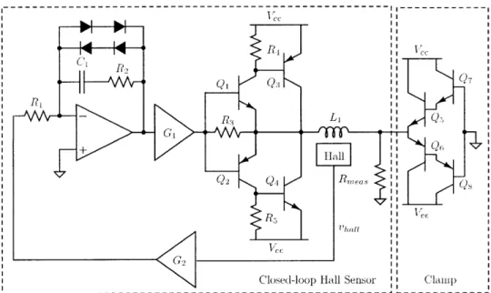
DAC + Gcomp OTA i Pi I Primary Current N2 iactual Comnpensation: Re Current P ---- - --- -- -- - -- N1 Closed-loop HInun Hall sen1sor' Hl N3 SADC Rmyeas LPF Clamp

Figure 2.4: Detailed block diagram of the prototype system.

current sensor and follows the overall design shown in Figure 2.2. The residual current measurement is a customized closed-loop Hall sensor. A compensation current driver consists of an auxiliary winding and a current driver. The compensation current icomp is driven anti-parallel to large input currents such that the effective total current imcas seen by the sensing element remains within its designated operating range. The mi-crocontroller coordinates and controls the system, performing calibration at startup and adjusting the compensation as necessary to keep the sensor at the desired operat-ing point [34]. The detailed block diagram of the whole system is shown in Figure 2.4.

2.2.3

Signal Reconstruction

The total input current factual is calculated from the instantaneous compensation current and sensor measurement as

factual

= kc -iconp + km -

imeas.

(2.5)

where the variables kc and km are calibration values determined by physical factors such as the number of turns on the sensing core and the amount of magnetic cou-pling between coils. The compensation current 1comp is generated by an operational

-transconductance amplifier (OTA), explained in Section 2.4.4. This current icomp is set by the microcontroller using a digital-to-analog converter (DAC) to generate a comnmand voltage, VDAC. The total compensation current is given by

t

comp kDAC ' VDAC, (2.6)

where the variable kDAC is determined by the OTA design.

Residual current is measured using a closed-loop Hall sensor, detailed in See-tion 2.4.1. This current imeas is read from an analog-to-digital converter (ADC) as the voltage VADC, and is given by

Imeas kADC ''VADC, (2-7)

where the variable kADC is determined by the sensor front-end design. Combining these equations, the complete reconstruction is

iactual c -kDAC - VDAC + km kADC

VADC-The constants can be simplified as:

tactual ks(VDAC s- + kr VADC), (2.8)

where the variable kr represents the ratio between the DAC command voltage and the corresponding change in ADC input voltage. and the variable k, represents a scaling to convert to actual current. This simplified form is used both for discussion and by the internal calibration and windowing procedures described in Section 2.4.5.

-Current (mA)

DAC output

ADC input

C I bi ; d t1+

10 bits (command)

6 bits (stable)

11 bits

S1 1V16

bits

Figure 2.5: Overlap of the DAC output, relating to compensation current, and the ADC input, relating to the residual measurement. The ranges and overlapped posi-tions are related to the parameters in (2.8). The combined result shows high accuracy over the full range.

2.2.4

Resolution and Range

The performance of the overall physically-windowed sensor system is determined by the parameters of its components. The ranges and resolutions of the compensation current and the residual measurement overlap, as depicted in Figure 2.5. In this example, the ADC is accurate to 11 bits over a range of 5 A, while the DAC command is accurate to 10 bits over a range of 160 A. The amount of overlap directly relates to the parameters k, and k, in (2.8).

A key requirement for physically-windowed sensing is that the compensation output must remain stable and predictable over the full desired system resolution. In Figure 2.5. this requirement is depicted as a dashed line on the DAC output. Here, for the lowest-order bits of the combined result to be accurate. each of the 210 possible DAC commands must result in a voltage stability of one part in 216. Certainly, a 16-bit DAC would suffice. However. only stability is needed, not accuracy. If a lower-resolution DAC is. or can be made to be. similarly stable in output, it is sufficient for

the sensor architecture. Using such a DAC may provide cost or performance benefits.

1

Given that the stability requirement is met, then the actual output voltage

VDAC

can be related to the DAC command x as

X

LOOKUP[X]

(2.9)

UDAC(\) oC 210 216

where LOOKUP[X] is a 21o-entry table that stores these 6 extra stable bits. This table can be populated by the micro-controller in a calibration step that uses the ADC input to determine the low-order bits of each DAC output.

2.2.5

Windowing

The front-end current measurement is "windowed" by the compensation current in

the sense that the compensation sets a particular current window as an operating

point, and the Hall sensor and ADC measure a small range of current in this window. The microcontroller has significant flexibility in the windowing approach. and the behavior can be adjusted based on expected bandwidth requirements and system parameters.

A basic approach to windowing is to continuously recenter the window so that the ADC measurement is zeroed; that is, the residual current is driven to zero after each sample. However, this requires that the OTA change its current output nearly continuously as the input signal changes, increasing the bandwidth requirements and potentially making the data less accurate if changes in compensation current are slow to settle. This extreme case fails to take advantage of signals that may be large amplitude low frequency content mixed with smaller amplitude high frequency contents. These types of signals are observed in the NILM environments and many

'The

prototype implementation in Section 2.4 simulates this stability by using a 16-bit DAC with fixed random low-order bits on a 10-bit command. The low-order bits are set by the micro-controller and can be adjulsted for testing purposes.

-other applications.

The approach illustrated by the reconstruction in Figure 2.3 is to change the DAC command when the residual current in the sensor approaches the limits of the ADC front-end. The compensation current will remain constant for small input signal changes, and only change for larger input signals that exceed the window range. For many input signals. this may allow the compensation to change relatively slowly, reducing bandwidth requirements for the compensation driver.

Other approaches are possible., particularly for loads with known character-istics. A predictive estimator in the micro-controller can perform an anticipatory change in the compensation current so that the residual sensor current would be ex-pected to fall within the sensor limits at the next sample interval. Such techniques can potentially increase the slew rate capability of the system.

2.2.6

Bandwidth

The bandwidth of the physically windowed sensor system depends on the input signal and its relation to the sensor window. There are two fundamental regions of operation: the first, within the windowed range of the residual current measurement, and the second, over the full range of the compensation current. For input currents that fall entirely within the window, the bandwidth performance of the system is equal to that of the residual current sensor front-end. as the compensation current is held constant. For full-scale input signals, the bandwidth is instead limited by how fast the compensation current can track the input change.

Maximum slew rate may be further affected by the windowing algorithm in use.

Once the residual current exceeds the range of the sensor window, the compensation

conunand must be adjusted. In the absence of prediction. the umicro-controller will not know the extent to which the residual current exceeds the window range, and will

be limited to stepping the compensation by one "window" worth of current at a time.

38-This. combined with the sampling rate of the residual sensor and the bandwidth of

di

the compensation driver, will set the maximum

that can be accurately tracked.

dt

For slew rates outside this limit, the subsequent front-end sample will still exceed the

window, and the micro-controller can report the potential inaccuracy as part of the

output data stream.

The bandwidth and slew rate limits are a function of the resolution, range. and bandwidth of the system components. Flexible trade-offs can be made, for example, by adjusting the system to increase kr in (2.8). This would have the effect of increasing the relative size of the sensor window, increasing the region in which the recorded signal retains full bandwidth, and increasing the maximum slew rate. Conversely. decreasing k, increases the overall resolution of the reconstructed signal.

2.3

Benefits and Motivation

In many physical systems, large-scale changes occur at relatively slow speed while small-scale details can change rapidly. For example, an electric motor draws a 60 Hz fundamental current from the utility, but it may be desirable to observe a principal slot harmonic (PSH) at several hundreds or thousands of Hertz to track the motor speed

[33].

These small, high-frequency details are superimposed on top of the 60 Hz current and need to be examined without saturating the sensor front-end. Conven-tional current sensors like the closed-loop Hall-effect sensor utilize a single compen-sation circuit to measure current. The physically-windowed sensing system., instead. divides the measurement into two subsystems, the compensation current driver and the residual current measurement. By dividing the problem and taking advantage of the fundamental differences between the requirements of the large-scale and small-scale measurements, the windowed system can utilize power and bandwidth trade-offs

in the design of design each subsystem. This section describes these trade-offs and

their design considerations.