How do sea-level curves influence modeled marine terrace sequences?

(1)

HAL Id: insu-02436871

https://hal-insu.archives-ouvertes.fr/insu-02436871

Submitted on 16 Nov 2020

HAL is a multi-disciplinary open access

archive for the deposit and dissemination of

sci-entific research documents, whether they are

pub-lished or not. The documents may come from

teaching and research institutions in France or

abroad, or from public or private research centers.

L’archive ouverte pluridisciplinaire HAL, est

destinée au dépôt et à la diffusion de documents

scientifiques de niveau recherche, publiés ou non,

émanant des établissements d’enseignement et de

recherche français ou étrangers, des laboratoires

publics ou privés.

How do sea-level curves influence modeled marine

terrace sequences?

Gino de Gelder, Julius Jara-Muñoz, Daniel Melnick, David Fernández-Blanco,

Hélène Rouby, Kevin Pedoja, Laurent Husson, Rolando Armijo, Robin

Lacassin

To cite this version:

Gino de Gelder, Julius Jara-Muñoz, Daniel Melnick, David Fernández-Blanco, Hélène Rouby, et al..

How do sea-level curves influence modeled marine terrace sequences?. Quaternary Science Reviews,

Elsevier, 2020, 229, pp.106132. �10.1016/j.quascirev.2019.106132�. �insu-02436871�

(2)

POSTPRINT PEER-REVIEWED, ACCEPTED & PUBLISHED BY QUATERNARY SCIENCE REVIEWS

This manuscript is a

postprint uploaded to EarthArXiv. It has been peer-reviewed and published in

Quaternary Science Reviews on the 01/02/2020, and has the DOI 10.1016/j.quascirev.2019.106132.

This postprint is also available via journal webpage with the “Peer-Reviewed Publication DOI” link to the

right. Authors welcome comments, feedback and discussions anytime.

(3)

How do sea-level curves inﬂuence modeled marine terrace

sequences?

Gino de Gelder

a,b,*

_{, Julius Jara-Mu~noz}

c

_{, Daniel Melnick}

d

_{, David Fern!andez-Blanco}

a,e

_,

H!el"ene Rouby

f

_{, Kevin Pedoja}

g

_{, Laurent Husson}

b

_{, Rolando Armijo}

a

_{, Robin Lacassin}

a

a_{Universit!e de Paris, Institut de Physique du Globe de Paris, CNRS, F-75005, Paris, France}

b_{ISTerre, CNRS, Universit!e Grenoble Alpes, 1381 rue de la Piscine, 38400, Saint Martin d’H"eres, France} c_{Institut für Geowissenschaften, Universit€at Potsdam, Karl-Liebknecht-Strasse 24, 14476, Potsdam, Germany} d_{Instituto de Ciencias de la Tierra, Universidad Austral de Chile, 5111430, Valdivia, Chile}

e_{Basins Research Group (BRG), Department of Earth Science & Engineering, Imperial College, Prince Consort Road, London, SW7 2BP, UK} f_!_{Ecole Normale Sup!erieure, Laboratoire de G!eologie, UMR, 8538, Paris, France}

g_{Laboratoire de Morphodynamique Continentale et C^oti"ere, CNRS, Universit!e de Caen, 14000, Caen, France}

a r t i c l e i n f o

Article history: Received 16 August 2019 Received in revised form 4 December 2019 Accepted 7 December 2019 Available online xxx Keywords: Quaternary Sea-level changes Global Coastal geomorphology Marine terraces

Landscape evolution models Corinth rift

a b s t r a c t

Sequences of uplifted marine terraces are widespread and reflect the interaction between climatic and tectonic processes at multiple scales, yet their analysis is typically biased by the chosen sea-level (SL) curve. Here we explore the influence of Quaternary SL curves on the geometry of marine terrace se-quences using landscape evolution models (LEMs). First, we modeled the young, rapidly uplifting sequence at Xylokastro (Corinth Rift; <240 ka; ~1.5 mm/yr), which allowed us to constrain terrace ages, model parameters, and best-fitting SL curves. Models that better reproduced the terraced topography used a glacio-isostatically adjusted SL curve based on coral data (for ~125 ka), and a eustatic SL curve based on ice-sheet models (for ~240 ka). Second, we explored the opposite end-member of older, slower uplifting sequences (2.6 Ma; 0.1e0.2 mm/yr). We find that cliff diffusion is important to model terrace sequence morphology, and that a hydraulic-model based SL curve reproduced observed terrace mor-phologies best. Third, we modeled the effect of SL noise with various amplitudes and wavelengths on our interpretations, finding that younger, faster uplifting sequences are less noise-sensitive and thus generally more promising for LEM studies. Our results emphasize the importance of testing a variety of SL-curves within marine terrace studies, and highlight that accurate modeling through LEMs may pro-vide valuable insight on climatic and tectonic forcing to Quaternary coastal evolution.

1. Introduction

Quantifying coastal uplift rates is essential for assessing tectonic

dynamics and estimating seismic hazard (e.g. Merritts and Bull,

1989;Shaw et al., 2008), and quantifying glacio-eustatic sea-level (SL) variations is fundamental to estimate global ice-sheet volumes and their spatio-temporal response to climate change (e.g.Chappell and Shackleton, 1986;Lambeck et al., 2002,2014). Sequences of paleoshorelines, resulting from the interplay between tectonic uplift and SL variations, cover much of the world’s coastline (Pedoja et al., 2011,2014) and thus provide a key archive to quantify both

processes (e.g.Bradley, 1958;Lajoie, 1986;Anderson et al., 1999). Paleoshorelines are markers of past SL position, reﬂecting global-to-regional tectonic and climatic processes since the Paleogene (Yamato et al., 2013;Henry et al., 2014;Pedoja et al., 2014), and are often expressed as marine terrace sequences. Marine terraces are relatively ﬂat, horizontal, or gently inclined surfaces of marine origin (Pirazzoli, 2005), occasionally covered by a layer of coastal sediments, and bounded inland by a fossil sea-cliff. Sustained land uplift over several SL cycles leads to staircase morphologies comprising a series of marine terraces separated by fossil sea-cliffs. Shoreline angles, at the intersection of terraces and paleo-cliffs, are commonly used as geomorphic indicators of past SL position and approximately time-equivalent to interglacial or interstadial SL highstands.

Marine terrace studies generally rely on terrace ages to

*Corresponding author. ISTerre, CNRS, Universit!e Grenoble Alpes, 1381 rue de la Piscine, 38400, Saint Martin d’H"eres, France.

E-mail address:Gino.De-Gelder@univ-grenoble-alpes.fr(G. de Gelder).

Contents lists available atScienceDirect

Quaternary Science Reviews

j o u r n a l h o m e p a g e :w w w . e l s e v i e r . c o m / l o c a t e / q u a s c i r e v

https://doi.org/10.1016/j.quascirev.2019.106132

(4)

constrain land uplift rates and/or relative SL history. Since typically only few ages within a terrace sequence are known (Pedoja et al.,

2014), studies commonly match undated terraces to Quaternary

SL highstands using modeling strategies based on either statistical metrics (e.g.Zeuner, 1952;Bowles and Cowgill, 2012;Roberts et al.,

2013) or landscape evolution models (LEMs; e.g.Quartau et al.,

2010;Melnick, 2016;Jara-Mu~noz et al., 2017,Pastier et al., 2019). These studies typically use a single SL curve, and do not always justify if the particular choice is based on resolution, timescale, geographic setting or otherwise. However, the choice of SL curve can introduce signiﬁcant uncertainties that might lead to biased results (e.g.Caputo, 2007;Sarr et al., 2019), as highstand estimates range in age by ~20 ka and SL elevation by ~30 m (Fig. 1). Recent studies have explored how different SL-curves inﬂuence correla-tions of shoreline angles to SL highstands (e.g.Caputo et al., 2010;

Pedoja et al., 2018a,b;Robertson et al., 2019), but the role of SL curves in LEMs and their impact on the full staircase morphology of a terrace sequence has not been investigated yet.

Here we apply a novel approach to model the development and age of marine terraces by investigating the inﬂuence of SL curves in LEMs. We test a spectrum of marine terrace sequences ranging from

young and rapidly uplifting to old and slowly uplifting sequences (Fig. 2). To test our approach we initially focus on two end mem-bers. For the ﬁrst end-member, we model the well-studied terrace

sequence of Xylokastro (Corinth Rift, Greece; Fig. 2), which is

rapidly uplifting (~1.5 mm/yr) and relatively young (~240 ka). This allows us to constrain terrace ages, uplift rates, and other model parameters using 14 SL-curves, of which one is corrected for Glacial Isostatic Adjustments (GIA). Simultaneously, we evaluate which SL-curves can best reproduce the observed morphology. For the other end-member, we model older (Quaternary-Pliocene), slower uplifting (0.1e0.2 mm/yr) terrace sequences. We focus on the SL curve signature of the Mid-Pleistocene Transition (MPT), instead of modeling a specific site, as there are no well-dated sequences covering the time-spans of interest. The MPT relates to the change from dominantly 40 ky to 100 ky climate cycles at ~1250e700 ka (Clark et al., 2006), associated with contrasting pre- and post-MPT morphologies in nature (Fig. 2; Pedoja et al., 2014). Lastly we investigate for both end-member cases the influence of SL noise, i.e. the complex arrangement of variable wavelengths and amplitudes defining SL oscillations. Known analogues for such SL noise are

meltwater pulses (e.g. Bard et al., 1996), Heinrich events (e.g.

Fig. 1. Compilation of selected SL curves. (a) The equatorial Pacific curve ofBates et al. (2014; curve 10, blue line) with the envelope of all other curves of our compilation (Table 1) in grey (see other curves in Supplementary Material). Boxes indicate age ranges for b and c (b) Elevation of SL highstands, with error bars as given in the original studies. Numbers indicate Marine Isotope Stage (MIS) and letters are substages as defined byRailsback et al. (2015). Black boxes encompass range of highstand estimates by the different SL curves (c) Zoom-in of SL curves since the Last Glacial Maximum (LGM), comparing the curves of our compilation (numbered 1e14) to the LGM-recent curve ofLambeck et al. (2014). MWP1A, MWP1B and 8.2 are meltwater pulses, YD ¼ Younger Dryas, H1 ¼ Heinrich Event 1. (For interpretation of the references to color in this figure legend, the reader is referred to the Web version of this article.)

(5)

Andrews, 1998) and the Younger Dryas (e.g.Fairbanks, 1989). These are identiﬁed over the last glacial cycle (e.g. LGM-recent curve of

Lambeck et al., 2014,Fig. 1c) and probably affect SL on all scales, but are not clearly reﬂected in SL curves focusing on time-scales of several 100 ka (Fig. 1c). Testing SL noise allows us to verify to what extent interpretations from our modeling approach are robust, and to what extent they may be limited by poorly constrained SL ﬂuctuations. The combined case studies allow us to explore the intrinsic relation between terrace sequence morphology and Quaternary SL cycles on a range of timescales, and provide general recommendations on the use of SL-curves in

marine terrace studies. 2. Background

2.1. Overview of sea-level curves

Sea-level (SL) changes are driven by variations in volume and shape of oceans, deﬁned as eustatic SL (ESL) change, as well as vertical land movement of coastal areas with respect to the sea surface, deﬁned as relative SL (RSL) change (Rovere et al., 2016a). During the Quaternary, glacio-eustasy has been a key long-term

Fig. 2. Marine terrace/rasa sequences. (a) Worldwide occurrence of marine terrace sequences (red), with white dots showing locations where rasas (wide polygenic fossil strandlines) of Early to Mid-Pleistocene age or older have been described in the literature. (b) Examples of rapidly uplifting marine terrace sequences, as shown in the literature. (c) Examples of slower uplifting and older marine terrace/rasa sequences. UR ¼ uplift rate. Proﬁles are based onAuthemayou et al., 2017; Merritts and Bull, 1989; Pedoja et al., 2006, 2018; Ward, 1988(For interpretation of the references to color in this ﬁgure legend, the reader is referred to the Web version of this article.)

(6)

mechanism driving SL changes (Bloom, 1971). Long-term climatic cycles drive the periodic decay and growth of large ice-sheets, associated with ESL rise and fall, respectively. To quantify past SL, the earliest published SL curves relied on the elevation of radio-metrically dated geologic/geomorphic SL markers, typically corals (e.g.Chappell, 1974;Bard et al., 1990). A dense set of coral data from several locations worldwide have resulted in well-constrained ESL estimates since the Last Glacial Maximum (LGM) at ~21 ka (e.g.

Lambeck and Chappell, 2001; Lambeck et al., 2014, Fig. 1c), but beyond this age, coral data become progressively sparser and

discontinuous, with larger age uncertainties (e.g. Braithwaite,

2016). As an illustrative example, the coral database of Hibbert

et al. (2016)contains 606 data points aged 0e21 ka (~30/ka), 1197 data points aged 21e130 ka (~10/ka), and 597 data points aged 130e850 ka (~1/ka).

Several methods have been developed to obtain longer and more continuous records of past SL by constructing SL curves from marine sedimentary cores. Evaporation favors the removal of ocean water containing the lighter oxygen isotope (16O) over the heavier oxygen isotope (18O). As a consequence, the oxygen isotope ratio in

seawater,

d

18OSW (16O/18O), can increase by ~1.5

‰

when large

amounts of water are stored within continental ice sheets during glacial periods. Most SL curves utilize this relationship between global ice-sheet volumes and

d

18OSW to estimate past SL. Different techniques have been developed to this end, each relying on a different set of assumptions and sedimentary cores from various locations (Table 1), resulting in a scatter of 10s of meters observed when comparing the different SL curves (Fig. 1).

2.1.1. Converting

d

18OC to

d

18OSW

The

d

18O of calcite (

d

18OC) is affected by both the

d

18OSW and by temperature. Assuming no post-depositional alteration has occurred, the use of independent proxies to quantify the

temper-ature component within

d

18OC, should result in more reliable

es-timates for the

d

18OSW conditions in which the calcite formed. ESL curves based on these assumptions typically use Mg/Ca ratios in ostracods (e.g.Dwyer et al., 1995) or foraminifera (e.g.Lea et al.,

2002) as temperature proxies. The

d

18OC is derived from benthic

(e.g. Elderﬁeld et al., 2012; Sosdian and Rosenthal, 2009) or

planktonic (e.g.Lea et al., 2002;Shakun et al., 2015) foraminifera.

The former mostly reﬂect the

d

18OSW and temperature of deep

water, whereas the latter reﬂects the sea surface temperature and the

d

18OSW of shallow waters. As the shallow seas are subjected to

stronger temperature variability, the conversion of benthic

d

18OC

to

d

18OSW is less inﬂuenced by local conditions than planktonic

d

18OC, and should be generally more reliable. An alternative way to convert

d

18OC to

d

18OSW was used byShackleton (2000), pairing a Paciﬁc

d

18OC with an Arctic record of atmospheric

d

18O trapped in ice-cores. For the ﬁnal step of converting

d

18OSW to ESL, studies typically use a linear conversion of 0.08e0.1

‰

m-1 (e.g.Shackleton, 2000;Elderﬁeld et al., 2012; Shakun et al., 2015), following cali-bration with a supposedly known ESL like the LGM at "130 m (Lambeck et al., 2014). This introduces additional uncertainties in the ﬁnal ESL estimate, since

d

18OSW varies spatially as a result of sensitivity to local precipitation, evaporation, and deep water forming processes.

2.1.2. Coral regression

Some studies have used coral datasets as benchmarks for

d

18O

records.Waelbroeck et al. (2002)constrained the direct relation-ship between coral-based paleo-ESL estimates for the last glacial

cycle (0e140 ka) and Paciﬁc/N-Atlantic

d

18OC records by ﬁtting

polynomial regressions. They separated the main glaciation from deglaciation interval and then applied their scaling to estimate ESL for the

d

18OC sections older than ~140 ka. The resulting ESL curve is a composite curve constructed from the most reliable sections of the different sedimentary cores. A similar approach has been used on longer time-scales using transfer functions for 10 cores spanning 0e5 Ma (Siddall et al., 2010;Bates et al., 2014), although at lower resolution (Table 1).Bates et al. (2014)apply their methodology to different oceanic basins, and given the major differences they found between Atlantic and Paciﬁc curves prior to the MPT, they conclude that their approach is not appropriate for this interval.

2.1.3. Inverse ice-sheet modeling

Sub-polar surface air temperature of the Northern Hemisphere plays a key role in two dominant factors affecting benthic

d

18OC: the ice sheet size and the deep-water temperature. Building on this

notion,Bintanja et al. (2005) used a global stack of 57 benthic

d

18OC records (Lisiecki and Raymo, 2005) to drive a 3D ice-sheet-ocean-temperature model. The model results in estimates for ice sheet volume, temperature and average ESL from 1070 ka to pre-sent. A similar approach was subsequently used in studies covering

2.7 Ma (Bintanja and Van de Wal, 2008) and even 35 Ma (De Boer

et al., 2010). The models over these longer timescales suffer from a lack of independent paleoclimate data to constrain their results,

Table 1

The different SL curves used in this study. Publication Duration

(ka)

Location Average Resolution original data (ka)

Method

1.Shackleton (200) 400 Equatorial Paciﬁc 1.3 d18Q-temperature correction other prosy

2.Lea et al 2002 360 Co cos ridge 3.0 dl8O- temperature correction other prosy

3.Waelbroeck et al 2002 430 Equatorial Paciﬁc & K-Atlantic

1.5 (best0.3) dl8O- coral regression 4.Bintanja et al 2005 1070 Global stack 1.4 (best 1) Inverse ice volume model 5.Bintanja and Van de Wal

2008 3000 Global stack 20 (best 1) Inverse ice volume model

6.Rohling et al., (2009) 520 Red Sea 0.8 (best 0.3) Hydraulic control models of semi-isolated basins 7.De Boer et al. , 2010 35000 Global stack 20 (best 1) Inverse ice volume model

8.Elderfield et al. , 2012 1575 South Pacific 1.1 d18O-temperature correction other prosy 9.Bates et al., (2014) 5000 Equatorial Pacifica _{28 (best 1.275)}

dl8O-coral regression

10.Grant et al. , 2014 500 Red Sea 0.2 Hydraulic control models of semi-isolated basins

11.Rohling et al., (2014) 5300 Mediterranean 1.0 Hydraulic control models of semi-isolated basins 12.Shakun et al., (2015) 800 Global stack 3.25 (best 1.5) d18Q- temperature correction other prosy

13.Spratt and Lisiecki (2016) 800 Global stack 1.0 PCA on 7 existing records

14. This study 130 Local GIA-corrected GIA-corrected, observation-calibrated ice volume models

(7)

and the authors point out that the simplicity of their ocean-atmosphere temperature coupling module and other modeling

assumptions lead to considerable uncertainties (Bintanja and Van

de Wal, 2008). 2.1.4. Hydraulic models

In semi-isolated basins like the Red Sea and the Mediterranean,

d

18OC is strongly inﬂuenced by both evaporation and exchange

with the open ocean, the latter closely related to sill depth and thus RSL.Siddall et al. (2003)used high-resolution

d

18OC records from

the Red Sea to reconstruct the history of water residence times. Through a hydraulic model of the water exchange between the Red Sea and the open ocean, they calculated RSL at the sill.Rohling et al. (2009)extended and improved this record using additional data, while Grant et al. (2014) improved the chronology through syn-chronization with an Asian monsoon record. Whereas the Red Sea records extend to ~500ka (Table 1),Rohling et al. (2014)applied the

same methodology to a Mediterranean

d

18OC stack to obtain an

RSL record for the last 5.3 Ma. However, the stability of Mediter-ranean Sea surface temperatures and relative humidity are difﬁcult to verify for this timescale, and so are the tectonic stability and isostatic response at the Gibraltar sill over several millions of years. In contrast to the other SL curves used in this study (Table 1), the hydraulic model curves represent RSL at the Hanish (Rohling et al., 2009; Grant et al., 2014) and Gibraltar (Rohling et al., 2014) sills, rather than ESL. Using glacial isostatic adjustment models at those two locations, the RSL is expected to scale approximately linearly with ESL, with factors of ~1.18 (Hanish; Grant et al., 2014) and ~1.23 (Gibraltar;Rohling et al., 2014).

2.1.5. Principal component analysis

Principal Component Analysis (PCA) is a statistical technique to reduce the number of variables of a dataset, while retaining the

most important trends within those variables.Spratt and Lisiecki

(2016)selected 7 SL records constructed with the methods out-lined above, and used PCA to identify the common ESL signal. The resulting stack was then scaled based on Holocene and LGM esti-mates. Although the signal-to-noise ratio in this PCA-curve should be much better than that of the individual curves, the approach may have resulted in a smoothing of the signal during interglacials, thus underestimating the SL elevation of brief highstands within those interglacials.

2.2. Modeling marine terrace sequences

We consider marine terraces as dominantly erosional features, as opposed to depositional (e.g. wave-built terraces) and constructional (e.g. coral reef terraces) paleoshorelines (as in

Pedoja et al., 2011), but note that there are conﬂicting deﬁnitions in the literature (e.g.Pirazzoli, 2005;Murray-Wallace and Woodroffe, 2014;Rovere et al., 2016b). Several studies explored the generation

of marine terrace sequences through LEMs.Anderson et al. (1999)

showed that wave dissipation is essential to the formation and preservation of marine terraces, and the formation of a terrace sequence is sensitive to a complex interaction of parameters, including SL history. They highlighted that the subsequent sub-aerial erosion of terraces is closely linked to stream incision rates, reﬂecting climatic conditions and limited by the rate of base-level

fall. Similar terrace formation models byTrenhaile (2002, 2014)

showed that terraces formed during interglacial and glacial pe-riods are more likely to be recorded in uplifting and subsiding landmasses, respectively, in agreement with natural examples (e.g.

Chappell, 1974;Ludwig et al., 1991). The author also modeled the positive correlation between uplift rates and the number of terraces preserved within a sequence, which had been previously

recognized in nature (Merritts and Bull, 1989;Armijo et al., 1996).

Along the same lines, LEMs of Melnick (2016)and Pastier et al.

(2019)emphasized that for low uplift rates, the continuous reoc-cupation of abrasion platforms, coupled to paleo-cliff diffusion, hinders the direct conversion of terrace elevations to uplift rates.

The amplitude and period of SL cycles have a distinct inﬂuence on the geometry of a modeled marine terrace sequence. Using synthetic SL curves, bothTrenhaile (2002)andHusson et al. (2018)

show that short-period, low amplitude SL oscillations before the MPT result in narrower terraces with smaller paleocliffs, compared to longer-period, higher amplitude SL swings after the MPT. Usage of the 3-Ma SL curve ofBintanja and Van der Wal (2008)resulted in similar conclusions, highlighting that the ~100-ky, ~120 m ampli-tude SL cycles since ~1 Ma lead to relatively more cliff erosion (Trenhaile, 2014). Similar tests for coral reef terraces by Husson et al. (2018) accentuated that SL noise is an inﬂuential factor in reef building, and infrequent, relatively long SL transgressions are important to the geometry of a sequence.

2.3. The coastal sequence at Xylokastro

The sequence of marine terraces at Xylokastro (Fig. 4) is located in the SE Corinth Rift (Greece). High uplift rates of ~1.2e1.5 mm/yr (Armijo et al., 1996;De Gelder et al., 2019), low sub-aerial erosion rates and thin cover of cemented coastal deposits have resulted in a

well-preserved sequence of 13 marine terraces (e.g.Dufaure and

Zamanis, 1979;Keraudren and Sorel, 1987;Armijo et al., 1996;De Gelder et al., 2019). The terrace sequence spans the last ~240 ka, and extends over an area of ~3 # 3 km, culminating at an elevation of ~400 m (Fig. 4b). The terraces were previously named after local towns (seeArmijo et al., 1996), but herein we assign a simpler name designation of TH (Holocene terrace) and T1-T12 (Fig. 4b). The T7 (New Corinth; ~175 m elevation) and T11 (Old Corinth; ~320 m elevation) terraces have been dated using both U/Th on solitary corals (Collier et al., 1992;Dia et al., 1997;Leeder et al., 2005), and IcPD dating of Pecten (Pierini et al., 2016). These studies correlate T7 and T11 to the Marine Isotope Stage (MIS) 5e (~125 ka) and MIS 7e (~240 ka) highstands, respectively. An inactive alluvial fan at ~200e230 m elevation caps T8 and T9, hindering our map of ter-races in this ~0.5 km2area (Fig. 4b).

3. Methods

3.1. Landscape evolution model

We use a LEM based on the wave erosion and wave energy

dissipation model formulated by Sunamura (1992), and further

developed by Anderson et al. (1999). The model simulates the

evolution of rocky coasts by the retreat of sea-cliffs, driven by wave erosion and resulting in the genesis of rocky shore platforms. The model assumes that the vertical seabed erosion rate is a linear function of the rate of wave energy dissipation against the seabed (Sunamura, 1992). The energy available at the sea-cliff to drive horizontal erosion is defined by the far-field wave energy remain-ing after wave energy dissipation (Anderson et al., 1999). The water depth profile dictates the spatial pattern of dissipation rate, expo-nentially increasing landwards as the water depth decreases. We use a 2D model setup formed by a planar shelf of given slope and assume that the rate of rock uplift is uniform. Cliff retreat starts at an initial rate and evolves as the platform is carved during SL os-cillations, which depends on the SL curve. Detailed description and equations can be found inAnderson et al. (1999).

(8)

3.2. Sea-level curves used

3.2.1. Sea-level curves selected from literature

We systematically selected from literature ESL curves that cover at least the last 3 major glacial cycles (~350 ka), and are based on data with a temporal resolution of <3 ka (Table 1). We also included three RSL curves based on hydraulic models. The 13 resulting SL curves (Table 1,Fig. 1) are subdivided into curves that; (i) convert

d

18OC to

d

18OSW (light blue,Fig. 1); (ii) use a regression analysis to ﬁx

d

18O curves to RSL estimates from corals (dark blue,Fig. 1); (iii)

are based on global ice-sheet modeling (green,Fig. 1); (iv) are based on hydraulic models of water exchange between an evaporative sea and the ocean (pink,Fig. 1); and (v) result from principal compo-nent analysis (PCA) of 7 other curves (brown,Fig. 1). More details are given inTable 1and section2.1.

3.2.2. Relative sea-level curve Xylokastro

ESL ﬂuctuations occur in response to the buildup and retreat of ice sheets, with local departures because of Glacial Isostatic Adjustment (GIA), i.e. solid earth and sea surface deformation un-der water and ice mass redistribution (e.g.Bloom, 1967;Walcott, 1972;Lambeck, 1995). As a ﬁrst attempt to account for the impact of GIA, we calculated a GIA-corrected RSL curve for Xylokastro, using the GIA models developed at the Australian National

Uni-versity (ANU) (e.g. Nakada and Lambeck, 1989; Johnston, 1993;

Lambeck et al., 2003,2014). The GIA model contains parameters describing both the deformation sources, i.e. the ice-volume dis-tribution history, and the behavior of the deformed object, i.e. the rheology of the Earth mantle. The ANU CALSEA code allows computation of the RSL for a given location and time back to the last interglacial. It includes all deformational, gravitational and rota-tional changes induced by the global ice history during the last glacial cycle, and accounts for the laterally variable rheology of the Earth mantle. The Earth model is not 3D, strictly speaking, but the effects of lateral variations are indirectly approximated by inverting regionally for the Earth mantle rheology and the ice and water volumes histories.

The ANU model is constructed using an iterative procedure. The ice volume history of each ice-sheet is solved regionally together with mantle rheology under the formerly glaciated areas by inversion of direct RSL observations (near-ﬁeld data from or within the former ice margins). Far-ﬁeld RSL data are separately inverted for total melted-ice volume and mantle parameters under oceanic and continental margins. The sum of individual ice-sheet volumes and the global volume are then compared and corrections are made to the different ice-volumes. The operation is iteratively updated

until reasonable convergence is obtained (Lambeck et al., 2001,

2010;2014,2017). Because there is even sparser direct observa-tional data before the last interglacial, the model is limited to 130 ka. We note that ignoring the MIS 6 ice-sheet conﬁguration prior to 130 ka, probably leads to additional RSL uncertainties on the order of a few meters (Dendy et al., 2017).

GIA models do not offer a highly detailed resolution when dealing with the Earth mantle viscosity. Three mantle layers (an elastic lithosphere and 2 visco-elastic mantle layers above and down the 670 km seismic discontinuity) and three combinations of rheologies (for continental, continental margin and oceanic man-tles) permit to predict Earth deformations due to ice melting (e.g.

Lambeck and Purcell, 2005;Lambeck et al., 2014;Lambeck et al.,

2017). Here, we adopt effective parameters for the Earth mantle

that reﬂect its behavior under a continental margin: a lithospheric thickness h ¼ 80 km, an upper-mantle viscosity

m

um ¼ 2 # 1020_{Pa s}

and a lower-mantle viscosity

m

lm ¼ 1022_{Pa s. These parameters are}

similar to those used within ANU models byLambeck and Purcell

(2005)for the Mediterranean region and bySimms et al. (2016)

for the US-Mexico Paciﬁc.

As the effective parameters used here are similar to those used bySimms et al. (2016)for the US-Mexico Paciﬁc coast, we expect uncertainties of the same order of magnitude (~5e10 m). Their uncertainty was estimated considering a range of parameters that reﬂect the lateral variations of the Earth’s mantle (more details in

Simms et al., 2016). We admit that the model assumptions and parameter choices are only rough approximations of reality, but a detailed investigation of GIA-model parameters is beyond the scope of this study. The purpose here is mostly demonstrative, and we note that uncertainties in the GIA-effects are relatively small in

comparison to the differences amongst SL curves (Fig. 1). The

calculated SL elevations for the RSL curve can be found in Dataset 2. 3.3. Modeling the coastal sequence at Xylokastro

We constructed a representative cross-section of the Xylokastro terraces to compare with the LEM simulated topography (Fig. 4a), by calculating average (i) shoreline angle elevations, (ii) terrace widths, (iii) terrace slopes and (iv) the modern rocky shore plat-form width. To determine shoreline angles, the intersection be-tween the marine terrace and its associated fossil sea-cliff, we used a 2-m resolution Digital Surface Model (DSM) developed from Pleiades satellite imagery (De Gelder et al., 2015,2019). From the DSM we calculated 100-m-wide swath proﬁles perpendicular to the fossil sea-cliffs and determined the shoreline angle positions

and elevations using the ﬁxed-slope method of TerraceM (

Jara-Mu~noz et al., 2016). We used the maximum swath proﬁle topog-raphy and the modern sea-cliff slope angle of 39$_±10$₍_{De Gelder}

et al., 2019) as a proxy for the slope of the paleo sea-cliff (Dataset S1). To approximate the terrace average width, we used the dis-tance between two successive shoreline angles (Fig. S1), since sub-aerial erosion of the paleo-cliffs has reduced the original terrace-width since they emerged. To estimate terrace slopes, we used the average slope of the modern terrace as less-eroded proxies for their older counterparts. To estimate the outer limit of the modern terrace, we assume that it has largely been carved during Holocene SL rise. Before ~12 ka (Moretti et al., 2004) the Corinth Gulf was a lake, its water exchange with the open sea limited by the 62 m deep Rion sill (Perissoratis et al., 2000). Assuming Holocene terrace carving started 12 ka at 62 m depth, and given an uplift rate of

~1.3 mm/yr (Armijo et al., 1996), the present depth contour

of "46 m should approximately represent the outer limit of the modern terrace (Fig. S1). Given the uncertainty in the bathymetry, and the unknown thickness of Holocene sediments on the carved

terrace (on the order of a few meters;Armijo et al., 1996), we

performed sensitivity tests on the width of the Holocene terrace of cases with both a 500 m shorter and longer terrace length (Fig. S2). We tied the cross-section shoreline angles of dated terraces T7 and T11 to the shoreline angles formed during the MIS 5e (~125 ka) and MIS 7e (~240 ka) highstands in the LEM. We ﬁxed LEM uplift rates to reproduce the observed average shoreline angle elevations, and varied initial erosion rate and initial shelf slope with steps of 0.1 m/yr and 0.25$_{, respectively. This allowed us to select the}

best-fitting pair of values that resulted in the lowest Root-Mean-Squared (RMS) misfit on both MIS 5e and MIS 7e timescales. The RMS misfit takes into account the full 2D-geometries of the modeled and observed profiles by comparing the vertical difference between both for every horizontal step (dx). To match modeled and observed terraces, we pick the observed terrace characterized by a shoreline angle elevation that is closest to that of the modeled terrace. Like the RMS-misfit, we consider the number of matched terraces as an indication for how well a SL curve can reproduce a terrace sequence. Our models used a spatial resolution of 2 m to

(9)

match our DSM. We used time-steps of 50 years, following sensi-tivity tests on the two highest resolution SL curves (Fig. S3): smaller time-steps give similar results. In the modeling, we assumed that the SL in Corinth did not get lower than the Rion sill (62 m depth) during the past 240 ka. We used a wave height of 3 m, based on the highest waves recorded between 2010 and 2015 at the Gulf of

Corinth with AVISO satellite altimetry measurements (Fig. S4;

https://www.aviso.altimetry.fr/). We choose to use the maximum wave height, because in nature most cliff retreat is typically ach-ieved during storms (e.g.Storlazzi and Griggs, 2000). Similarly, the upper limit of a terrace is usually considered as the storm swash height (Rovere et al., 2016b;Lorscheid and Rovere, 2019). Sensi-tivity tests for wave height and sill depth show that those param-eters do not strongly affect our results (Fig. S4).

3.4. Modeling old, slow uplifting sequences

To constrain marine terrace geometries for older, slower uplifting sequences, we model the formation of marine terrace sequences over the whole Quaternary (2.6e0 Ma) using the four

longest SL curves of our compilation (Bintanja and van de Wal,

2008;De Boer et al., 2010;Bates et al., 2014;Rohling et al., 2014). In our modeling strategy, we use a relatively low initial slope of 4$

and an uplift rate of 0.1 mm/yr, consistent with an approximate average of the examples shown inFig. 2c. We used an initial sea-cliff erosion rate of 0.6 m/yr, consistent with our average estimate for Corinth (see results), and included a 0.1 m2/yr sub-aerial cliff diffusion rate to obtain a more realistic sequence morphology over this timescale.

3.5. Inﬂuence of noise in sea-level curves

To test the inﬂuence of noise in SL curves on both end-member type marine terrace sequences, we start with a curve composed of 40 ky-period, 65 m-amplitude sine function to describe SL over the 2.6e1 Ma interval, and a 100 ky-period, 130 m-amplitude sine function over the 1-0 Ma interval. We then add noise to this SL curve with amplitudes of 4, 10 or 25 m spaced every 1, 5 or 20 ky, using the rand function in MATLAB®. We use the same erosion rate and initial slope as in section3.4, test cases with and without a sub-aerial cliff diffusion rate of 0.1 m2/yr, and test both 0.1 and 1.5 mm/ yr uplift rates over 2.6 and 0.4 Ma, to compare with the MPT and Xylokastro case studies, respectively.

4. Results

4.1. Modeling the coastal sequence at Xylokastro

The systematic comparison of observed topography in the Xylokastro marine terraces sequence and their modeled topog-raphy allows us to 1) assess possible age ranges for undated ter-races, 2) quantify the governing parameters of terrace formation, and 3) evaluate the best-ﬁtting SL curves by means of the number

of matched terraces and the RMS misﬁt. InFig. 3we show four

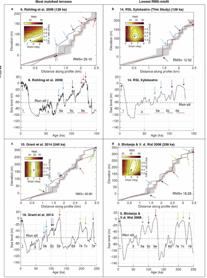
examples of our analysis, displaying the curves resulting in the most terraces (Fig. 3a and c) and lowest RMS misﬁts (Fig. 3b and d) over ~125 ka (Fig. 3a and b) and ~240 ka (Fig. 3c and d).Fig. S5

contains the results for the other tested SL curves. Correlation of modeled shoreline angle elevations to the nearest shoreline angles results in different ages estimates as a function of SL curve (Fig. 4a). Most curves suggest a chrono-stratigraphy in which: T2 was formed during MIS 5a (~70e85 ka); T3 during MIS 5a or MIS 5c (~92e107 ka); T4 and T5 during MIS 5c; T6 and T7 during MIS 5e (~115e128 ka); T9 during MIS 7a (~190e205 ka); T10 during MIS 7a or 7c (~210e225 ka); and T11 during MIS 7e (~235e242 ka). T1 and

T8 were only reproduced by SL curves 2 and 3, respectively, but relative to the other terraces would logically have an age of MIS 5a or younger (T1), and MIS 8 or MIS 9a (T8).

The uplift rate (Fig. 4c), initial erosion rate (Fig. 4d) and initial slope (Fig. 4e), vary strongly between different SL curves, and for the two different timescales. Despite this variation, the overall average values remain similar over time (Fig. 4cee). The number of matched terraces for the different curves has a broad range for both ~125 ka (2e6 terraces) and ~240 ka (4e7 terraces) timescales, but none of the selected curves recreate the observed number of 11 successive terraces (Fig. 4f). Plotting the number of matched ter-races against the temporal resolution of each SL curve shows a strong correlation between higher resolution curves and a larger number of matched terraces (Fig. S6), although higher curve reso-lution does not correlate with lower RMS misfits (Fig. S6). No SL curve gives consistently good results in terms of RMS misfits, but we note that for ~125 ka the two lowest misfit curves are based on corals (dark blue; 3 and 14 inFig. 4g). Over the same timescale, the curves based on hydraulic models (pink; 6, 10 and 11 inFig. 4g) give consistently high misfits.

We compared the ESL and the RSL curves calculated by the ANU

model (see section3.2.2) to highlight how GIA corrections

inﬂu-ence our approach (Fig. 5). The difference between these two

curves is typically on the order of several meters (Fig. 5b), and the GIA-correction of the ESL curve improves the RMS misﬁt by > 3 m (Fig. 5a), while reproducing an extra terrace. The GIA-corrected curve is also the overall best-ﬁtting curve over the last ~125 ka. 4.2. Modeling the Mid-Pleistocene Transition (MPT)

Lower uplift rates (0.1 mm/yr) in the 2.6-Ma models (Fig. 6)

generally result in fewer terraces being formed than at Xylokastro (Fig. 4). At such uplift rates, only terraces formed during the max-ima of interglacial highstands (MIS 5e, 7e etc.) are preserved. The effect of the MPT is most pronounced when modeling the curve of

Rohling et al. (2014), resulting in 2 rasas (wide polygenic fossil strandlines) formed before the MPT and 5 marine terraces after the

MPT (Fig. 6a, e). Sequences produced by other SL curves do not

show a similarly clear contrast before and after the MPT. The curve with the most (Bates et al., 2014) and least (Rohling et al., 2014) pronounced change in cyclicity around the MPT (spectrograms in

Fig. S7), correspond to the least and most prominant change in sequence morphologies, respectively (Fig. 6). Additional tests with alternate uplift rates, erosion rates and initial slope are character-ized by variations in the shape of staircase sequences (Fig. S8), but consistently show the lowest ratio between terraces/rasas pre-served before and after the MPT in the case of the hydraulic curve (Rohling et al., 2014).

4.3. Inﬂuence of noise in sea-level curves

We estimated the effect of various degrees of noise added to synthetic SL curves for slowly uplifting coastlines (~0.1 mm/yr) (Fig. 7). The reference profile has no noise (black lines,Fig. 7a) and portrays a prominent cliff that separates an upper, pre-MPT section of narrow terraces with small cliffs, from a lower, post-MPT section of wider terraces with higher cliffs. Cliff-diffusion completely smoothens all pre-MPT cliffs, and partly smoothens post-MPT cliffs (thick black line,Fig. 7a). Adding a relatively moderate 4 m of noise spread out every 20 ky has a significant influence on the sequence morphology with respect to the reference profile, and leads to variations in terrace width and cliff heights both pre- and post-MPT. With higher noise amplitudes and lower noise wavelengths, the contrast between the two intervals (pre- and post-MPT) is less clear. The cliff separating the two intervals becomes less prominent,

(10)

Fig. 3. Examples of modeling the Xylokastro terrace sequence. (a) For the most matched terraces over ~125 ka; (b) for the lowest RMS-misfit over ~125 ka; (c) for the most matched terraces over ~240 ka, and; (d) for the lowest RMS-misfit over ~240 ka. In profile plots (above), red lines show average-derived terrace topography (see methods) with 1s

uncertainty (grey envelope), black lines the modeled topography, and arrows indicate which SL highstand corresponds to which shoreline angle. Dashed lines connecting shoreline angle of modeled and observed shoreline angles indicate the correlation used forFig. 4a. In the SL plots (below), numbers indicate MIS and letters are substages as deﬁned by

(11)

and the overall width of the pre-MPT section increases relative to the width of the post-MPT section. In general, the addition of cliff diffusion (thick lines inFig. 7a) results in fewer and often composite terraces (rasas), especially for the pre-MPT section. Using the same curves over 400 ka with an uplift rate of 1.5 mm/yr (Fig. 8) results in very minor differences in comparison to the reference proﬁle, and these are only clearly visible for the SL curve with 25 m, 1 ky wavelength noise. For noise amplitudes of 10 and 25 m with 1 and 5 ky wavelengths, respectively, the overall shape of the terrace

sequence is similar but minor sub-levels form. Overall the noise tests indicate that terrace morphology is more affected by noise with higher noise amplitudes and shorter noise wavelengths. Se-quences with lower uplift rates are more sensitive to the inﬂuence of noise.

5. Discussion

Here we re-evaluate different aspects of our analysis towards a

Fig. 4. Overview of all Xylokastro terrace models. (a) Profile of the terrace sequence. The black line shows average-derived terrace topography (see methods) with 1suncertainty (grey envelope) and range of possible terrace ages indicated by the different SL curves, including median age (m) and number of curves (n) reproducing a given marine terrace. (b) Map of Xylokastro marine terrace sequence. SA ¼ shoreline angle. (ceg) Different parameters and outcomes resulting from finding the lowest RMS-misfit over the two time-scales, shown for all 14 RSL curves. Models over 125 ka and 240 ka are shown in red and green, respectively. Numbers below plot correspond to SL curve numbering and colors ofFig. 1, and are sorted by type of SL curve for easy comparison. Solid and dashed lines indicate average values and 1suncertainty. (c) Uplift rates required by the different SL curves to match the correct elevations of the dated T7 (red) and T11 (green) terraces. (d) Erosion rate for lowest RMS-misfit result. (e) Initial slope for lowest RMS-misfit result. (f) Total number of terraces for lowest RMS-misfit result. (g) Lowest RMS-misfits. (For interpretation of the references to color in this figure legend, the reader is referred to the Web version of this article.)

(12)

unified objective: understanding how SL curves affect modeled marine terrace sequences. We first discuss results from the Xylo-kastro sequence, which is a short and well-defined sequence, and therefore appropriate as a test site at high resolution. We then discuss the MPT results and the possible pitfalls associated with longer time-scale modeling, including the influence of SL noise, and compare both end-member type marine terrace sequences. Finally, we conclude with some general recommendations and perspec-tives on using SL-curves in marine terrace analyses based on our findings.

5.1. Modeling coastal sequences: the Xylokastro lessons 5.1.1. Approach limitations

Modeling tests on the Xylokastro terrace sequence reveal the complexity of reproducing as many terraces as observed in nature, either as a consequence of model assumptions and/or SL curves

used. The relatively simple model used (Anderson et al., 1999) does not take into account the abrasive effect of sediments, long-shore drift, or coastal sediments on the terraces. Additionally, the far field wave energy is considered constant in our models, even though it probably varies within glacial-interglacial climate cycles and thus impacts erosion rates. Although these might all influence terrace sequence geometry, implementing such processes within our model is beyond the scope of this study, given that the influ-ence of the chosen SL curve would remain of primary importance in

any model. Models byTrenhaile (2002,2014)included a more

so-phisticated parameterization of wave regime and coastal cliff retreat, but the author concluded that the results were generally

consistent with those of Anderson et al. (1999). Therefore, we

expect a more detailed set of cliff erosion parameters would not have changed our results significantly. Our simple model assump-tions of using a constant and uniform uplift rate, erosion rate and initial shelf slope for Xylokastro appear justified, as none of those parameters have significantly changed on both timescales (Fig. 4cee). Even if variations in the initial slope existed within the Xylokastro sequence and affected the resulting terrace geometry, by averaging the terrace width and cliff height over a 1e5 km wide area we expect to have accounted for such possible lateral varia-tions. Furthermore, the widest terraces in the Xylokastro sequence are also the widest terraces up to ~25 km further east (Armijo et al., 1996; De Gelder et al., 2019), suggesting that terrace width is influenced more strongly by SL curves than by variable initial slopes.

The temporal resolution may restrict the number of marine terraces produced, given the limitations of the SL curves used. The amount of SL peaks within a curve logically limit the number of terraces that can be formed. As such, relatively lower-resolution

curves with few SL peaks like the smooth curve ofDe Boer et al.

(2010), lead to few distinct terraces. The curves with the highest resolution (Rohling et al., 2009; Grant et al., 2014;Fig. S5) show that sharp and short duration peaks within a SL curve can result in extra terraces, as conﬁrmed by the positive correlation between resolu-tion and number of matched terraces (Fig. S6). Detailed studies of MIS 5e show that multiple peaks may have occurred even within one interglacial (e.g.Hearty et al., 2007;Blanchon et al., 2009;Kopp et al., 2013;O’Leary et al., 2013; Murray-Wallace and Woodroffe,

2014), although we note that other studies have disputed this

(e.g.Long et al., 2015;Barlow et al., 2018). Most of our selected ESL and RSL curves do not reﬂect interglacial SL variability, indicating that short-wavelength peaks may be underrepresented in most SL curves and limit the number of matched terraces for the Xylokastro sequence.

5.1.2. Approach advantages

Our analysis of the Xylokastro sequence provides clear advan-tages over more classic analyses that do not include modeling (e.g.

Merritts and Bull, 1989;Armijo et al., 1996;Strobl et al., 2014). Using a range of curves is essential to check the robustness of uplift rate estimates and possible correlations between SL highstands and undated marine terraces (e.g.Caputo, 2007;Yildirim et al., 2013;

Pedoja et al., 2018a,b). Our approach expands on these studies by not only using shoreline angles and SL highstands, but also the full terrace sequence geometry and complete SL curves. In this manner, we take advantage of the model prediction that higher highstands and longer periods of preceding SL rise lead to wider terraces. Such geometrical trends, with some highstands leading to wider ter-races, are also observed in nature (Regard et al., 2017). Additionally, our modeling approach allows for an evaluation of parameters like erosion rates and initial slopes, and their evolution through time, with possible climatic and paleogeographic implications.

Another advantage is that we can analyze which SL curves better

Fig. 5. Xylokastro modeling results for the CALSEA ESL curve and GIA-corrected RSL curve. (a) Profile comparison for lowest RMS-misfit modeling results. The red line shows average-derived terrace topography (see methods) with 1suncertainty (grey envelope), the black dashed line shows the modeled topography with the CAL-SEA ESL curve, and solid black line shows the modeled topography with the GIA-corrected RSL curve. Arrows indicate which shoreline angle corresponds to which SL highstand in frame b. (b) The two SL curves, in which numbers indicate MIS and letters are substages as defined byRailsback et al. (2015). (For interpretation of the references to color in this figure legend, the reader is referred to the Web version of this article.)

(13)

reproduce the geometry of a studied marine terrace sequence. For example, it is reasonable that for the Xylokastro sequence, curves based on coral data (dark blue inFig. 4g) have lower misﬁts on a 125 ka than 240 ka timescale, since the data on which they are based become sparser with increasing age. Possibly the lower resolution of the curve inBates et al. (2014; curve 9 inFig. 4g) with respect to

Waelbroeck et al. (2002; curve 3 inFig. 4g) results in higher RMS misﬁts over 125 ka. Considering curves based on the conversion of

d

18OC to

d

18OSW over 125 ka (light blue inFig. 4g), the

benthic-based curves (1 and 8 inFig. 4g) have lower RMS-misﬁts than the

planktonic-based curves (2 and 12 inFig. 4g). This possibly relates to the stronger temperature variability in shallow seas (see Back-ground section), although over 240 ka the planktonic-based curve ofShakun et al. (2015, curve 12 inFig. 4g) has the lowest RMS misﬁt. For the inverse ice-sheet modeling curves (green inFig. 4g), the lowest-resolution and longest timescale curve (35 Ma; curve 7 in

Fig. 4g) has a much higher RMS-misﬁt than the other two, sug-gesting it is less appropriate for short timescales of 125e240 ka. The

hydraulic model RSL curves generally have high RMS misfits (pink inFig. 4g) on both timescales, whereas the PCA-based curve has relatively low RMS misfits on both timescales (curve 13 inFig. 4g). Overall, the four SL curves with lowest RMS misfits over 240 ka (curves 4, 5, 12 and 13) are all based on globally distributed data-sets, which argues in favor of using such curves.

We infer that the curves with the lowest RMS misﬁts are the most appropriate to describe SL variations at Xylokastro to ﬁrst order, but their lack of temporal resolution produces a lower number of terraces than observed in nature. In contrast, the two

highest-resolution SL curves (6, 10 in Fig. 4f) produce more

matched terrace levels, but their high RMS misfits suggest that they are less appropriate to describe first-order SL variations (Fig. 9a). The noise tests with high uplift rates (Fig. 8) support this inference: at high uplift rates, the overall sequence geometry is mostly a function of first-order SL variations. The type of short-wavelength noise represented within high-resolution SL curves can lead to an increase in terrace levels, but does not significantly change the

Fig. 6. Model results on Quaternary (2.6 Ma) timescale. (a) Modeled geometry of the long-term sequences, dashed lines indicating the MPT. Inset shows typical morphology for a Quaternary staircase sequence, modiﬁed fromPedoja et al. (2014). (bee) Modeled SL curves, with lettered arrows indicating SL highstands that result in preserved terraces in frame a.

(14)

diffusion and thin lines without cliff diffusion. (b) Modeled synthetic SL curves, characterized by a 40 ky, 65 m amplitude sine function before 1 Ma, and a 100 ky, and a 130 m amplitude sine function after 1 Ma. Noise amplitudes are 4, 10 and 25 m, increasing to the right, and noise spacing 1, 5 and 20 ky increasing downwards.

(15)

overall staircase morphology except for unrealistically extreme values (Fig. 8; amplitude 25 m, wavelength 1 ka).

5.1.3. Glacio-isostatic adjustments

The use of GIA-corrections in the analysis of past SL has become

increasingly popular (e.g.Raymo and Mitrovica, 2012; Creveling

et al., 2015; Simms et al., 2016), although less common in the analysis of paleoshorelines. GIA-corrections are highly uncertain before the LGM given our limited knowledge of past ice-sheet conﬁguration, discontinuous RSL data availability and un-certainties in ice model parameters. Despite these unun-certainties, the GIA-corrected RSL curve ﬁts the terrace sequence morphology better than any of the other curves for our study of the Xylokastro

sequence (Figs. 3 and 4g), encouraging the use of such GIA

cor-rections within coastal terrace studies. However, we note that the improvement that is achieved through the GIA correction is rela-tively minor in our study (3 m in RMS-misﬁt;Fig. 5) in comparison to the variations between different ESL curves (21 m in RMS-misﬁt;

Fig. 4g). This suggests that applying GIA-corrections to all ESL curves would not change the general pattern of higher and lower RMS-misﬁts when comparing SL-curves. Along the same lines, we conclude that GIA-corrections may be useful, but the use of a wide variety of SL curves is more important to terrace analyses, at least for Mediterranean locations like Xylokastro.

The hydraulic model Gibraltar/Hanish RSL curves were calcu-lated for a different location, so to be used in Xylokastro, ideally they should be converted to ESL curves and then GIA-corrected to create Xylokastro RSL curves. Following the RSL to ESL conversions ofRohling et al. (2014)and Grant et al. (2014), the ﬁrst step implies a decrease in glacial/interstadial SL of several meters, and following our ESL to RSL conversion, the second step implies an increase in glacial/interstadial SL of several meters (Fig. 5). Therefore, we expect these corrections to roughly balance out, and to have a relatively small impact on the results.

5.2. The MPT, SL noise and quaternary evolution of staircase coastal landscapes

Continuous re-occupation and/or removal of older terraces at

low uplift rates leading to relatively few terraces (Fig. 6) is

conﬁrmed by both natural observations (e.g. Merritts and Bull,

1989; Armijo et al., 1996) and previous LEM studies (Trenhaile, 2002,2014; Melnick, 2016,Pastier et al., 2019). Based on global

observations of Neogene-Quaternary strandline sequences,Pedoja

et al. (2014)suggested that the change in cyclicity frequency from 40 to 100 ka during the MPT is probably causing a contrast between wide rasas before the MPT, and narrower and better individualized marine terraces after the MPT (inset inFig. 6a). Within this context, modeling with low uplift rates over 2.6 Ma (Fig. 6) suggests that SL curves based on hydraulic models (Rohling et al., 2014) and corals (Bates et al., 2014) are the most and least successful, respectively, in recreating globally observed sequences. However, this result should be interpreted with care, given the long timespan of these models and the inherently increasing uncertainty of model assumptions.

Additional processes may become relevant at sites that exhibit a terrace sequence over the entire Quaternary or longer timescales. In cases where uplift is driven by magmatic or tectonic processes, some studies have noticed that land uplift is episodic and spatially variable instead of continuous (Saillard et al., 2009;Ramalho et al., 2010;Walker et al., 2016). We note that such episodic uplift would have similar effects as the SL noise we test (Figs. 7 and 8), both inﬂuencing RSL in an unpredictable manner. Other studies have

focused on the inﬂuence of dynamic topography to RSL (e.g.Conrad

and Husson, 2009and references therein). Over ~125 ka this may contribute to a few meters of uplift/subsidence (Austermann et al.,

2017), whereas over Pliocene timescales this may increase to a few tens of meters (Rowley et al., 2013). As such, both variable uplift rates and dynamic topography can be relevant to studies that aim at reconstructing past ESL from individual sites, or estimating the tectonic contribution to uplift/subsidence rates. For our MPT case study however the difference in terrace morphology pre- and post-MPT appears to be a global feature irrespective of geodynamic setting (Fig. 2; Pedoja et al., 2014). Therefore neither a variable uplift rate nor dynamic topography is likely to drive morphological contrasts within terrace sequences on a global scale.

The differences amongst SL curves after the MPT (Fig. 1) warrant caution on their reliability, and even more so for the SL curves covering longer timespans (Fig. 7). SL noise like meltwater pulses and Heinrich events is not well reflected in most SL curves on post-LGM timescales (Fig. 1c), and is probably reflected with even less accuracy on longer timescales. We note that GIA-corrections like those applied for Xylokastro, on the order of a few meters, can similarly be considered as ‘noise’ within local studies. Different methods for SL-reconstruction rely on assumptions for which reliability is difficult to verify over long timescales, given the limited independent data to compare against. For all four SL curves used on Quaternary timescales there are methodological concerns (see Background section), and as a consequence, differences amongst the curves are more striking pre-than post-MPT. Post-MPT oscillations are all on the order of ~100 m amplitude (Fig. 6bee), but pre-MPT oscillations in SL occur with amplitudes of ~25 m (De Boer et al., 2010,Fig. 7c) to ~75 m (Rohling et al., 2014,Fig. 6e). Within LEM studies, this makes the resulting geometry of a terrace sequence highly uncertain. It is also striking that for slowly uplifting sequences, noise in a SL curve can have a major impact on sequence morphology even for perturbations of 4 m amplitude (Fig. 7). These perturbations are small in comparison to meltwater pulses and Heinrich events (Fig. 1c). As such, SL noise appears to be an important controlling parameter for the geometry of a terrace sequence, especially for slowly uplifting sequences, yet it is difficult to quantify.

Our results align with those of Trenhaile (2002, 2014), with

more wave erosion resulting in a relatively wider sequence post-MPT, although in our models we show that increasing noise may decrease the relative contrast in sequence width pre- and post-MPT (Fig. 7). There appears to be a variation in such relative widths in nature, as well as in the prominence of the cliff separating the two (Fig. 2). Given enough sites, perhaps the inﬂuence of changing climate cycles, noise, uplift rates and initial slopes for full Quater-nary sequences can be deciphered, but given the larger number of variables we suspect this would result in a multitude of non-unique solutions.

The observed contrast in pre- and post-MPT morphology is possibly due to the speciﬁc arrangement of SL noise components,

with theRohling et al. (2014)curve quantifying those most

suc-cessfully (Figs. 6 and 9b). Alternatively, cliff diffusion provides an easy explanation to the ﬁrst-order morphological difference before and after the MPT. Smaller amplitude, shorter period SL ﬂuctua-tions form smaller cliffs and narrower terraces, which diffuse more easily into wide rasas (Figs. 6 and 9b), and obscure the original sequence morphology. Comparing these two mechanisms, the main difference in resulting sequence morphology lies in the slope of pre-MPT rasas in comparison to post-MPT terraces: whereas the rasa formed using theRohling et al. (2014)curve has a similar slope to the terraces, a diffused series of narrow, small cliff terraces will result in a rasa with a steeper slope than the post-MPT terraces (Fig. 9b). In natural sites the rasa slope can be easily compared to the terrace slope to distinguish the two mechanisms. In our four examples (Fig. 2c), only the Mancora (Peru) sequence has a clearly steeper pre-MPT slope, pointing towards the importance of

(16)

SL-m2/yr cliff diffusion. (b) Modeled synthetic SL curves, characterized by a 100 ky, 130 m amplitude sine function. Noise amplitudes are 4, 10 and 25 m, increasing to the right, and noise spacing 1, 5 and 20 ky increasing downwards.

(17)

noise arrangement. Thorough morphological analysis of more long-lasting, slowly uplifting sites would be required to verify this hypothesis.

Our models show that sequences with faster uplift rates, like Xylokastro, are much less sensitive to noise than slowly uplifting sequences (Figs. 7 and 8). Considering the natural availability of terrace sequences there appears to be a trade-off by which the faster uplifting sequences tend to represent shorter time-intervals (Pedoja et al., 2014). Following the terrace degradation models of

Anderson et al. (1999), an easy explanation would be the inﬂuence of river incision, with higher uplift rates implying a faster base-level drop and more aggressive channel incision. In the case of Xylo-kastro this appears to be true; although rapid uplift seems to have taken place since ~1 Ma (Armijo et al., 1996; Nixon et al., 2016;

Fern!andez-Blanco et al., 2019), the associated river incision has

removed terraces older than ~240ka (Fig. 4b). Following our

modeling results for Xylokastro, the MPT, and relative inﬂuence of SL noise, we conclude that within the spectrum of naturally observed sequences, the shorter-timescale, faster uplifting sites offer more potential to reconstruct ﬁrst order SL variations using LEMs.

5.3. Sea-level curves in marine terrace analysis: recommendations and perspectives

Selecting an appropriate SL curve within marine terrace analysis is not trivial (Caputo, 2007), and can have a signiﬁcant inﬂuence on uplift rate estimates (e.g.Pedoja et al., 2018a,b). Based on our case

Fig. 9. Schematic representation of main results (a) In the case of rapidly uplifting, young sequences (~1.5 mm/yr and ~240 ka in the Xylokastro case study), a higher resolution SL-curve leads to more matching terraces, whereas a SL-curve with better first-order shape of RSL leads to a lower RMS-misfit with the observed sequence morphology. We list some of the SL-curves that roughly fall into the four categories illustrated for the Xylokastro case study. (b) In the case of slowly uplifting, old sequences (~0.1 mm/yr and ~2.6 Ma in the MPT case study), the observed contrast in sequence morphology pre- and post-MPT can be the result of (left) a contrasting sensitivity to cliff diffusion for narrow terraces with small cliffs formed pre-MPT and wider terraces with larger cliffs formed post-MPT, or (right) the specific arrangement of SL-noise pre-and post-MPT, possibly better constrained by theRohling et al. (2014)RSL-curve.

(18)

studies, we can put forward some general recommendations. It is of primary importance to check a variety of SL curves, whether using LEMs or statistical methods. Assessing the reliability of different types of SL curves requires a thorough evaluation of assumptions and uncertainties that are difﬁcult to quantify. Yet, within each type of SL curve it is easier to select the most appropriate curve: logical and justiﬁable choices can be made based on the resolution of the original data, time-span, and spatial variability that the SL curve is based on. For some well-studied highstands like MIS 5e and MIS 11c (e.g. Dutton et al., 2015), direct estimates from RSL compilations provide additional estimates. GIA-corrections can improve local RSL predictions, but at latitudes relatively far from ice-sheets, like Xylokastro, these are probably of secondary importance. Using LEMs has advantages over more classical methods, as they take into account the full geometry of a terrace sequence and full shape of a SL curve. Testing several SL curves through LEMs allows for an assessment of (1) possible ages for undated marine terraces, (2) physical parameters involved in the formation of marine terrace sequences, and (3) the (types of) SL curves which are the most consistent with the geometry of the studied sequences. Marine terrace sequences that are relatively young and rapidly uplifting appear more promising for LEM studies than older, slower uplifting sequences for several reasons. Firstly, the assumption in long-term SL curves that the relation between

d

18O and paleoclimate proxies, ice sheet dynamics and/or hydrodynamic conditions can be linearly extrapolated up to >1 Ma, is highly uncertain (see Background). Secondly, for lower uplift rates the sequence morphology becomes more sensitive to SL noise like meltwater pulses, Heinrich events and local GIA-effects, and thirdly, variations of uplift rates and dynamic topography are more likely to occur over longer timescales.

For the MPT case study we ﬁnd thatRohling et al. (2014)RSL

curve best reproduces observed sequence morphologies. For our Xylokastro case study, the RMS-misfits indicate that the best-fitting SL curves are two SL curves based on coral data for 0e125 ka, and four ESL curves based on globally distributed datasets for 0e240 ka (Fig. 9a). These inferences are based on one sequence of 13 terraces, and thus the SL curves that have lower misfits here might not have the same performance elsewhere. To overcome this bias, similar

analyses can be applied to many locations worldwide (Fig. 2a;

Pedoja et al., 2014). The rapidly increasing availability of high-resolution topography, like the Xylokastro DSM used in this study, is a crucial development for such a comparison, and could allow for a global perspective on best-ﬁtting SL curves from marine terraces. One step further would be to use LEMs to directly reconstruct ESL, through the inversion of terrace sequence morphology with a probabilistic approach. Simultaneous analysis of both uplifting and subsiding sequences could constrain both interglacial and glacial SL, and provide unique new SL constraints.

6. Conclusion

For our objective of understanding how SL curves affect modeled marine terrace sequences, we draw the following con-clusions from our Xylokastro, MPT and noise case studies:

1. Using a LEM to reconstruct marine terrace sequences and testing several different SL curves allows for a detailed analysis of possible terrace ages, model parameters and the SL-curves that best reproduce a sequence, while utilizing the full geome-try of a terrace sequence.

2. Comparing the modeled and observed terrace geometries of rapidly uplifting sequences, the RMS misﬁt indicates how good the ﬁrst-order shape of a SL curve is for that particular site, whereas the number of matched terraces depends on the

resolution of a SL curve. For the Xylokastro case study, we ﬁnd the lowest RMS misﬁts for coral-based SL-curves over ~125 ka, and SL-curves based on globally distributed datasets for ~240 ka, whereas high-resolution hydraulic model curves result in the most matched terraces on both timescales.

3. GIA-corrections can provide improvements for modeling terrace sequences, but are relatively minor in comparison to differences amongst SL curves at Mediterranean sites like Xylokastro. 4. The contrasting terrace sequence morphologies pre- and

post-MPT can either be the result of cliff diffusion and/or the spe-ciﬁc noise arrangement within a SL curve. The dip of the rasa with respect to the terraces can be used in nature to distinguish between both mechanisms.

5. Older, slower uplifting sequences are generally less favorable for LEM modeling, because (i) SL-curves over >1 Ma timescales are increasingly uncertain, (ii) terrace morphology is more sensitive to SL-noise for low uplift rates, and (iii) uplift rates are less likely to be continuous because of tectonic and/or dynamic topog-raphy variations.

6. Young, rapidly uplifting sequences with well-preserved mor-phologies provide an opportunity for reconstructing past SL through LEM modeling.

Declarations of competing interest None.

Acknowledgments

GdG, DFB, RA and RL acknowledge funding from the People Programme (Marie Sklodowska-Curie Actions) of the European Union’s Seventh Framework Programme under the ITN project ALErT (Grant FP7-PEOPLE-2013-ITN number 607996). GdG also acknowledges a postdoctoral grant from the Centre National d’Etudes Spatiales (CNES, France). DM acknowledges financial support from the Millennium Nucleus The Seismic Cycle Along Subduction Zones funded by the Millennium Scientific Initiative (ICM) of the Chilean Government (grant 1150321) and Chilean National Fund for Development of Science and Technology (FON-DECYT; grant 1181479). JJM acknowledges financial support from DFG grant JA 2860/1-1. We thank Kurt Lambeck and Anthony Pur-cell for sharing the ANU GIA model and code. We thank Arthur Delorme for assistance in producing the DSM, Riccardo Caputo for SL curve data, Stephanie Bates for her spectral analysis code, and Marco Meschis and Jennifer Robertson for fruitful discussions. Numerical computations for the DSM were performed on the S-CAPAD platform, Institut de Physique du Globe de Paris (IPGP), France. This study contributes to the IdEx Universite de Paris ANR-18-IDEX-0001. This is IPGP contribution 4096.

Appendix A. Supplementary data

Supplementary data to this article can be found online at

https://doi.org/10.1016/j.quascirev.2019.106132. Data

Pleiades satellite imagery was obtained through the ISIS and Tosca programs of the CNES under an academic license and is not for open distribution. On request, we will provide the DSM calcu-lated from this imagery to any academic researcher who gets

approval from CNES (contact isis-pleiades@cnes.fr quoting this

paper,lacassin@ipgp.frin copy). The altimeter products were pro-duced and distributed by Avisoþ (https://www.aviso.altimetry.fr/), as part of the Salto ground processing segment. The MATLAB® code