Adhesive properties of silicone resins

Adhesive properties of Silicone Resins

by

Bruno Charon

Ing6nieur de l'Ecole Polytechnique (France) Promotion 1994

Submitted to the Department of Materials Science and Engineering in Partial Fulfillment of the Requirements for the Degree of

Master of Science in Materials Science and Engineering

at the

Massachusetts Institute of Technology September 1998

C 1998 Massachusetts Institute of Technology

All rights reserved

Signature of Author ... ...

Department of Materials Science

Certified by ... ...

Accepted by ... ...

and Engineering August 7, 1998

i J. McGarry rofessor of Polymer Engineering Thesis Supervisor

... . .. . .. . ... ... ... .... . 0 . . Linn W. Hobbs John F. Elliott Professor of Materials Chairman, Departmental Committee on Graduate Students

Adhesive Properties of Silicone Resins

Bruno Ch6ron

Submitted to the Department of Materials Science and Engineering on August 7, 1998 in Partial Fulfillment of the Requirements for the Degree of Master of Science in Materials

Science and Engineering

Abstract

An experimental study on adhesive properties of Phase I rubber toughened rigid silicone resins was performed to determine the possibility of an application such as structural adhesives. Single-lap shear tests were used to study several parameters, such as the thickness of the joint, the overlap length, the behavior at high temperature and a comparison with different adhesives.

Results suggest that a 10% KPE / 6% Cab-O-Sil® _{modified silicone resin shows}

optimal adhesion for sandblasted plates and a 0.1 mm thick joint, whereas such an optimum has not been observed for the untoughened resin. For small overlaps, the failure criterion is the shear strength of the resin, whereas for laps over 20 mm, it is the applied load. Toughened silicone resins behave well at high temperatures, as the strength of the joint is half as small between 150 and 2500_{C as it is at room temperature. Furthermore, no}

degradation has been noticed for exposures up to 2000_{C and up to 500 hours, but the resin}

starts decomposing after 10 hours at 2500_{C. Last, comparison with other commercial glues}

proves that the studied toughened silicone resin provides a relatively strong bond, between the performance of epoxy glues and cyanoacrylate adhesives.

Thesis Supervisor: Frederick J. McGarry Title: Professor of Polymer Engineering

Table of Contents

ABSTRACT 2

TABLE OF CONTENTS 3

LIST OF ILLUSTRATIONS AND FIGURES 6

LIST OF TABLES 8 ACKNOWLEDGEMENTS 9 I. BACKGROUND 10 A. Joining 10 1. Adhesion 10 a) chemical bonding 11 b) electrostatic bonding 12 c) physical bonding 14 d) mechanical bonding 17 2. Adhesive joints 18 B. Silicones 21 1. Chemistry of silicones 21 a) synthesis of silicones 22 b) Vulcanization 23

2. Properties and applications of silicones 24

a) Chemical properties 25

b) Physical properties 27

C. Rubber toughening 29

1. Particle insertion 29

2. Modification of the chemical structure 30

II. DESCRIPTION OF THE EXPERIMENT 31

A. Preparation of the specimen 31 1. Preparation of the plates 31

2. Preparation of the resin 33

3. Preparation of the joint 36

4. Curing 37

5. Cutting the samples 39

B. Testing 40

1. Measuring the specimen 40

2. Apparatus used 41

III. RESULTS 43

1. Observation of tested specimen 43

a) load-displacement curves 43

b) surface of the adherend 45

c) fracture pattern 47

2. Study of some properties of the joints 52

a) thickness of the joint 52

b) length of overlap 53

c) heat resistance 55

d) stress transfer 58

e) comparison with other adhesives 59

IV. DISCUSSION: 61

1. Thickness of the joint: 61

2. Length of overlap 63

3. Heat resistance 64

5. Comparison with other glues

V. CONCLUSION

VI. FUTURE EFFORTS

BIBLIOGRAPHY

67

68

List of Illustrations and Figures

Figure 1: Energy and force of interaction between two molecules, according to

Lennard-Jones potential 12

Figure 2: wetting of a solid surface 14

Figure 3: idealized liquid adhesive 15

Figure 4: squeezing of a drop between two parallel plates 16 Figure 5: some common engineering adhesive joints (from Ref. [1]) 19 Figure 6: "Performance" of several types of joint (from ref. [27]) 20 Figure 7: step-polymerization of siloxanes (example of PDMS) 22 Figure 8: ring-opening polymerization (example of D4) 23 Figure 9: mechanism of addition (through vinyl group) 24 Figure 10: "adhesion" of silicones (here a silane) onto a surface containing hydroxyl

groups 26

Figure 11: assembly of samples 37

Figure 12: curing cycle 38

Figure 13: cutting: the samples are cut along the dot-lines, making 7 specimen 39

Figure 14: measuring the specimen 40

Figure 15: typical load-displacement curve for the specimens tested 44 Figure 16: load-displacement curves from a same sample (=5 specimens) 45

Figure 17: SEM micrograph of sandblasted aluminum 46

Figure 18: SEM micrograph of anodized aluminum 46

Figure 19: SEM micrograph of anodized aluminum (magnification of Figure 18) 47 Figure 20: Pattern of cohesive failure observed by Adams and Peppiatt for lap shear joints

with filet 48

Figure 21: SEM micrograph of a "dendritic" fracture surface 50

Figure 23: SEM micrograph of the transition between smooth surface and fractured resin51 Figure 24: SEM micrograph of the smooth region of a "dendritic" failure surface 51 Figure 25: Influence on thickness on strength of the joint 53 Figure26: maximum load supported as a function of the overlap 54 Figure27: maximum average shear stress supported as a function of the overlap 55 Figure 28: Influence of temperature and length of exposure on strength of a lap-joint (only

the average result is displayed) 57

Figure 29: Comparison of different adhesives 60

List of Tables

Table 1: strength of some covalent bonds. 11

Table 2: Binding energies for various types of interactions (adapted from [9]) 13

Table 3: surface energy of some polymers 14

Table 4: Average shear strength at failure (in MPa) for single lap joints tested at a given temperature after a given amount of time exposed to high temperatures 56

Acknowledgements

I wish to thank Professor McGarry for his guidance and help which made this work fruitful and valuable.

I would like to thank the 3M Company and Dow Corning Corporation who sponsored this study and without whom this work would not have been possible.

I wish to express my gratitude to Arthur and Stephen Rudolph, who took great care of the cutting of the samples, and gave great advice too.

I was very pleased to work in Professor McGarry's group. I had wonderful moments talking and working with Dr. Carmen Bautista, Yuhong Wu, Dr. Dave Zhou, and Mike Li. I am deeply grateful to Evelyn Hum for carefully reading my thesis and suggesting

sentences which sound English.

Many thanks to DMSE's staff, and especially Diane Rose, Gloria Landahl and Ann Jacoby. They are always nice and helpful.

Many thanks to my friends, Jeff Hiller and Gael Gioux. Their fresh view of my problems helped me many times, but most of all, their sense of humor will be missed. I wish them good luck for the end of their studies.

I would like to take this opportunity to thank my parents and my family for their care, love and support throughout my life. I must not forget Mr. and Mrs. Guedat, Mrs. Dusseaux, and Mr. Schneider, who had a strong impact on my education, and without them, I would not be where I am now.

Last but not least, many thanks to my girlfriend, Oksana Chikova. Her love, tenderness and support are invaluable gifts. Despite of the miles separating us, she always knew how to comfort me in hard times. I hope that life will be easier for both of us now.

I.Background

A. Joining

1. Adhesion

Manufacturing objects often requires joinng different parts. This can be done in several ways. A vast majority of bonds are done through welding, fastening and gluing. Welding provides a strong bond, but is restricted to metals. Fastening is a very simple way of bonding. It requires nails, staples, screws or bolts, and it is relatively efficient. However, adhesive joints are at least as efficient as mechanical fasteners. As a matter of fact, a line of glue is more economic, shows a better stress distribution, whereas fasteners tend to be heavier and concentrate stresses around them1_.

Therefore adhesion is a widely used process for joining. Yet, it is not quite fully understood. Many models have been developed at different levels (from the atomic level up to the macroscopic level), but none of them describes reality adequately. This paragraph will briefly review some of the most used models. A model is typically suitable in a given situation, but not in others, showing that adhesion might be actually a combination of those models. The most common models can be classified within one of the four following

categories:

- chemical bonding

- electrostatic bonding

- physical bonding

a) chemical bonding

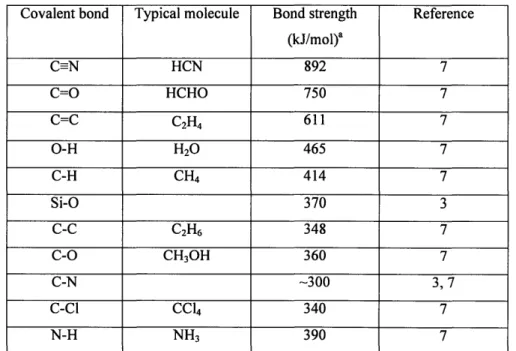
The most obvious way to bind two molecules together is to create a covalent bond between them. Polymers, when they polymerize, harden because of the covalent bonds that have formed. But chemical bonding seldom happens between two different materials. Indeed, it is known that bond strength is usually an order of magnitude below what it would be if there were chemical bonds2. Nevertheless, it is believed that covalent bonds can form between adhesives with isocyanate groups and hydroxyl groups, or between epoxide adhesive and amine groups3. Another possibility is to use coupling agents, which will act as a medium between the adhesive and the adherend and bind both of them. Silane coupling agents are widely used4,56, especially for the coating of glass fibers. In such cases, the ultimate bond strength might be obtained. Table 1 provides some common covalent bond strengths.

N-H NH₃ 390

Table 1: strength of some covalent bonds.

Covalent bond Typical molecule Bond strength Reference (kJ/mol)a C-N HCN 892 7 C=O HCHO 750 7 C=C C2H4 611 7 O-H H20 465 7 C-H CH4 414 7 Si-O 370 3 C-C C2H6 348 7 C-O CH30H 360 7 C-N ~300 3, 7 C-Cl CCl4 340 7

b) electrostatic bonding

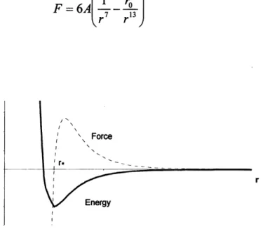
Atoms and molecules interact between each other. They can share electrons as in the case of covalent bonding, but they can have weaker interactions. Those are electrostatic interactions, due to the Lennard-Jones potential:

U=-- 2 r,2

Where A is a constant, r the intermolecular distance, and ro the intermolecular distance at equilibrium.

As

dU F = dU

dr

We get an expression for Van der Waals forces between molecules:

F=6A r7 r

SForce

' r

r

Energy

Figure 1: Energy and force of interaction between two molecules, according to Lennard-Jones potential

This potential can be illustrated by various types of forces. Molecules can be adsorbed onto surfaces8. Polar molecules can act as dipoles and interact with other polar molecules (dipole-dipole interaction), but can also create a dipolar moment to molecules which were initially apolar, or increase their initial polar moment (dipole-induced-dipole interaction)9_{. Hydrogen has a specific role, and can lead to relatively strong interactions,}

especially with highly electronegative atoms such as oxygen, chlorine, fluorine, nitrogen or groups (i.e.: -CC13, -CN). But apolar molecules can interact with each other too. This is the London Dispersion Force'0, 11, 12, 13, which has been explained with simple words by

Hirschfelder et al.14_:

"At any instant the electrons in molecule a have a definite configuration, so that molecule a has an instantaneous dipole moment (even if it possesses no permanent electric moment). This instantaneous dipole in molecule a induces a dipole in molecule b. The interaction between these two dipoles results in a force of attraction between the two molecules. The dispersion force is then this instantaneous force of attraction averaged over all instantaneous configurations of the electrons in molecule a "

An order of magnitude of interactions discussed here above is given in Table 2.

Type of force Energy, kJ/mol reference Chemical bonds: Ionic 590-1047 9, 15 Covalent 63-712 9, 16 Metallic 113-348 9, 17 Intermolecular force Hydrogen bonds up to 50 9, 18 Dipole-dipole up to 21 9 Dispersion up to 42 9 Dipole-induced-dipole up to 0.02 9

c) physical bonding

liquid

Solid surface SL 7sv

Figure 2: wetting of a solid surface

When a liquid is disposed onto a solid surface, it tends to take the shape of a droplet. The contact angle between the droplet and the surface depends on the surface tension of the materials. They are all linked with Young's equation:

YLV COS9 = YSV - YSL

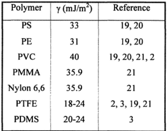
Many factors influence the wetting angle. As shown in the previous equation, the surface tension (or surface energy) of the liquid or of the solid surface are important parameters. Surface tensions of some polymers are mentioned in Table 3. But surface roughness can increase the wetting angle too, while impurities (dust) can decrease it.

Polymer y (mJ/m2) Reference PS 33 19, 20 PE 31 19, 20 PVC 40 19, 20, 21, 2 PMMA 35.9 21 Nylon 6,6 35.9 21 PTFE 18-24 2, 3, 19, 21 PDMS 20-24 3

Obviously, the more the liquid that wets the solid surface, the stronger the bond will be. Indeed, with a small wetting angle, the adhesive will spread and cover then a significant area. On a smaller scale, if the wetting angle is small, the liquid will tend to come to intimate contact with the adherend and thus will increase the true surface of contact.

A liquid adhesive can bridge the adherends as on Figure 322 and form capillary adhesion20_{: the adhesive wets both adherends and forms a concave meniscus. Assuming}

that the surface of contact with the adhesive is circular with a radius R and a thickness 2r, the difference of pressure in the adhesive (PI) and in the air (Pa) is roughly:

P/ - Pa = YLV I -I)

Both adherends are held together with a pressure P1- Pa. It should be related to the

strength of the joint. A closer look at the equation shows that the smaller r (i.e. the thinner the joint) is, the stronger the bond. A typical example of capillary adhesion is Johansson Blocks. Machinists use those steel blocks which have a very flat surface as measurement standards. When those blocks are very close to each other, it is very difficult to separate them by tension, because adsorbed water vapor acts as an adhesive.

2r

Figure 3: idealized liquid adhesive

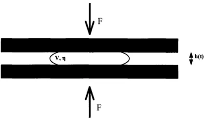
Viscosity can be involved in the process of adhesion. Let us consider a drop of liquid squeezed between two parallel plates (see Figure 4). Due to the viscosity of the liquid (rl), the displacement of the plates (initial separation of the plates hi, and final separation hf), the force applied on those plates (F) and the time for a given displacement (t) are related by the Stefan equation:

3r7V2 (ii1

F.t = 3

47( h h4₎

Where V is the volume of the drop.

But this equation remains valid for the separation of the plates. Consequently, it means that a large force is required to separate the plates in a small amount of time. On the opposite, a small load can break a joint, but it will take a very long time. A very viscous liquid will make a strong joint, as well as a very thin joint. Among others, this equation explains why it is easy to adjust a joint when the glue has not dried, whereas it is almost impossible once the adhesive has hardened.

F

h(t)

d) mechanical bonding

When an adhesive penetrates the pores of the adherend, or wets a very rough surface and then solidifies, it creates two "interpenetrating networks" which lock the adhesive and the adherend together. That is why surface preparation is critical in order to get a strong joint. Most surface preparations used tend to follow this concept"3'23 Sandblasting creates a very rough surface, whereas anodizing creates a porous layer at the surface of the metal.

The diffusion theory of adhesion is somewhat similar to mechanical bonding. Indeed, polymer chains of the adhesive can diffuse within the adherend and thus create a relatively strong bond. This theory has been mainly developed by Voyutskii24 _and

Vasenin25'26_{. But this requires that the temperature be higher than the glass transition}

temperature of the polymeric adhesive. The consequence is that diffusion bonding is restricted to the adhesion of similar materials (two metals or two polymers, although it is seldom possible). This method of bonding is not widely used. It is mainly restricted to some polymers (and metals). For example, PMMA can bind two pieces of PVC, under certain conditions3. Wake evaluates the acceptance of this theory on p. 72 of reference

2. Adhesive joints

Imagination and creativity of men has led to various shapes and types of joints. Some of them are shown on Figure 5. Their efficiency varies widely and depends on the geometry of the joint, among other factors. Hart-Smith27 _{has shown that scarf and}

stepped-lap joints look like the most efficient types of joint. Nevertheless, properties of adhesives are still tested with single-lap or peel joints. This might be surprising at first glance, since Figure 6 shows that lap joints are very weak. But lap-joints are easy to prepare, and they are close to "real-life" joints. Moreover, they provide results which can be used for the design of structures such as airplanes, because they will give a conservative performance of the adhesive.

Single-lap joints have been extensively studied. Several theories have emerged. Adams reviewed most of them in reference [28]. Among them, it is necessary to mention the linear elastic theory (which will be used later in the present study), Volkersen's Analysis (shear lag model) and Roland and Reissner's Analysis1' 29 (which takes into

account the bending of the specimen). However, those analysis are not really satisfactory, due to peel stresses at the edges of the lap-joint, and higher precision can only be reached with Finite Element Analysis.

a) Single-lap b) Double-lap c) Scarf d) Bevel e) Step f) Butt strap g) Double butt-strap h) Butt i) Tubular ap

I

FALURES SHOWN

SRPRESEN TADHEREND T LMT HICKNESS

Figure 6: "Performance" of several types of joint (from ref. [27])

w = ah-" OULP INT

prparameters. For mostthe adhesives presenting elastoplastic properties, the value of m testing

B. Silicones

Silicon is one of the most abundant element on Earth, 27.61% of earth's crust according to Clarke33. Nowadays, silicon is more and more used. It has become a multi-billion dollar business thanks to the appearance of computers, but its use is not restricted to ships, glass, sand and other cements. Over the years, polymers containing silicon have developed and started competing with organic (carbon-based) polymers.

1.Chemistry of silicones

Silicon is the fourteenth element. In Mendeleiev's table, it is located just below Carbon. Thus, both elements are tetravalent and have a similar electronic configuration: [He] 2s2 _2p2 _{for C and [Ne] 3s2 3p}2 _{for Si. Those similarities have lead many}

science-fiction writers to imagine worlds where silicon would have replaced carbon...

However, silicon forms a very strong bond with oxygen, "one among the most

durable of covalent bonds between elements", as described by Liebhafsky34. As a matter of fact, Si-O bond seems somewhat stronger than C-C bond (see Table 1). This feature has lead to focus on polysiloxanes (silicones), and attempts to compare them with organic polymers.

a) synthesis ofsilicones

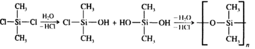
There are two main ways of synthesizing silicones. The first consists in the hydrolysis of diorganodichlorosilanes. This step polymerization leads to unbranched silicones and a by-product (HC1). Close control of experimental conditions (concentrations of reactants, removal of HCl, temperature...) is necessary to obtain the wished degree of polymerization.

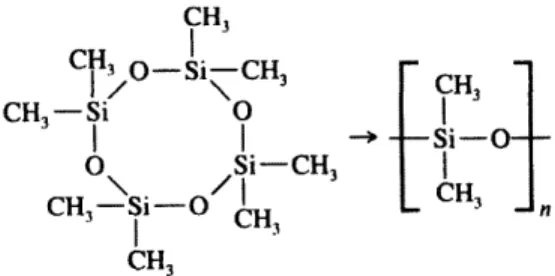
The second way for synthesizing silicones is to use ring-opening polymerization. The monomers most widely used are hexamethylcyclotrisiloxanes (D3*) and octamethylcyclotetrasiloxane (D4), which can be produced through the step polymerization described previously. It is possible to use either cationic polymerization or anionic polymerization, provided adequate catalysts are used35,36. Ring-opening polymerization allows to reach higher degrees of polymerization and thus high molecular weights. Another advantage of ring-opening polymerization is the low polydispersity.

CH, CH3 CH, CH

I n110 I I -n~o

Cl-Si-Cl -- CI-Si-OH + HO-Si-OH --- -O-Si

I - I I - I]C I

CH, CH, CH, CH

Figure 7: step-polymerization of siloxanes (example of PDMS)

Polyorganosiloxanes are made up of the following structural units: * M-unit (mono-functional): R3SiOl/2

* D-unit (di-functional): R2SiO

* T-unit (tri-functional): RSiO3/2

CH3 CHO-SiCH, CH3W-Si 0 O Si-CH₃ CH3-Si-O CH CH, -+ _CH3d -Si-O-I

I

Figure 8: ring-opening polymerization (example of D4)

b) Vulcanization

Provided that the unbranched siloxane has some tri- or quadro-functional groups, it can undergo branching. This creation of T or Q units can lead to the formation of a three-dimensional network. Those chemical links (cross-links) may be completed by "mechanical" links (entanglements). Polmanteer37 _{describes four vulcanization methods.}

First, at elevated temperatures, peroxides can create free radicals which will generate the cross-linking reaction. The second method, still for an elevated curing temperature , is hydrosilation. Then, for room-temperature vulcanization, he separates two-part systems and one-part systems. But two main chemical reactions underlie this classification38_:

Me

MeSiH + CH2 CH-Siv Me

Figure 9: mechanism of addition (through vinyl group)

A condensation reaction happens between two silanol groups and the by-product is often water, but not exclusively: it can yield an alcohol (e.g. ethanol) or a carboxylic acid (e.g. acetic acid).

The kinetics of an addition reaction is usually faster than a condensation reaction. Nevertheless, addition reaction brings some "weak" carbon-carbon bonds in the backbone

structure, and it tends to lower the temperature of decomposition of the polymer.

2. Properties and applications of silicones

Silicones have been a wide area of research throughout the century39_{. This has led}

to a better understanding of their properties, and to numerous applications4 0_'4 1_{: surfactants,}

a) Chemical properties

The main property of silicones is their chemical inertness, due to the strong Si-O bond.

However, since silicones can be formed by hydrolysis, they might undergo the reverse reaction. It has been reported that silicones can be attacked by steam42_{. As a result,}

the silicone undergoes rearrangements (especially formation of cyclic polysiloxanes: D3,

D4...). Fortunately, this does not affect the properties of the material.

The backbone of siloxanes is relatively flexible. As a matter of fact, the bond angle Si-O-Si varies between 120' and 1500, depending on the substituents36. Moreover, Si-O bond can rotate freely43.

Si-O bond proves to be polar, and thus may be attacked by acids or bases. Incorporation of phenyl groups in the polymer decreases this drawback. Another property related to polarity and free rotability of the Si-O bond is water repellency. All organic substituents move to the same side of the backbone and hence create a polar side (oxygen atoms) which tends to align onto a polar substrate, whereas the non-polar groups (Si-R) repel water.

Unbranched polysiloxanes are commonly called silicone fluids. But when they have tri-functional groups, silicones can undergo vulcanization. Depending on the degree of linking, such silicones will become elastomers, or resins when they are highly cross-linked. Although many articles are published on silicone rubbers, it seems that nothing has been done so far on rigid silicone resins besides the work of Zhu4 4

.

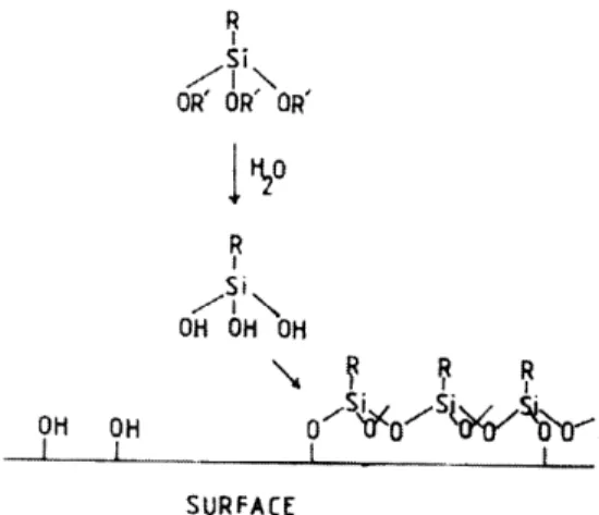
Hydrosilation does not need two organosilicon compounds to occur. Siloxanes and silanes can bind this way to surfaces which have hydroxyl groups (see Figure 10). This is especially interesting for the adhesion of silicones to metals which have an oxide surface layer. Silane coupling agents are used to promote adhesion45_,38 _{and RTV (room}

R

OR' OR' OR'

R

OH OH OH

SURFACE

Figure 10: "adhesion" of silicones (here a silane) onto a surface containing hydroxyl groups

Due to the strength of the Si-O bond, silicones can stand high temperature without decomposing (up to 2500C). Hence, silicones can be used as fire retardant. Addition of silica (SiO2) can enhance this property47 48. Attempts have been made to incorporate

silicones within organic polymers in order to increase their fire resistance. Those hybrid organic-inorganic polymers were either polymer functionalization48 or copolymerization4 9. Results of these studies were encouraging. But more promising is the use of silicone as adhesives that can withstand high temperatures50'51.

Last, silicones show a good resistance to oxidation and ozonation. Phenyl groups as substituents enhance this property. Thus, silicones are suitable for aerospace applications4 6.

b) Physical properties

Silicones have typically a low melting point (around -50'C) and a low glass transition temperature (around -120C)36_{, due to the flexibility of their backbone.} Branching and phenyl substituents can improve this property even more. As a consequence, silicone tubing is widely used, since it remains flexible at low temperatures.

The latter application illustrates another feature of silicones: temperature almost has no influence on some of its electrical or mechanical properties, compared to materials which have similar properties.

Due to their low surface tension (Table 3 shows that only PFTE, a.k.a. Teflon, has a lower surface energy than PolyDiMethylSiloxane), silicones will spread and wet surfaces very well. Many applications derive from this: non-stick applications (mold release coatings on tire molds and milk cartons, lubricants, etc.), and water repellency (seals in the bathroom, shoe and clothes protectors, etc) are the most common.

Last, silicones are used as surfactants which help improve paints and show a good resistance to radiation.

c) Miscellaneous

On average, silicone can be considered a good electrical insulator, although it may vary. This property can be explained by the protection that the methyl group provides to the SiO bond, as well as the hydrophobic properties mentioned before. Then, it is not

surprising to see silicones as a protective layer in electrical wires, or in circuit boards. Medicine is another wide field for silicones. Their chemical inertness and their lack of toxicity make them well accepted by human bodies. They are some of the few materials compatibles with living systems, and can replace some articulations, cartilage37

Most mechanical properties (adhesion, rubbery behavior) of silicones are consequences of physical and chemical properties, and thus have been previously discussed.

C. Rubber toughening

Nowadays, most polymers manufactured are rubber-toughened52_{. As a matter of}

fact, polymers were usually extremely brittle, and incorporation of rubber allowed to erase this drawback and can significantly improve their impact strength. Two different ways of rubber toughening have been developed so far. The first one consists of incorporating rubber particles within the polymer and blending the mixture. On the other hand, it is sometimes fruitful to modify the chemical structure of the polymer by inserting rubbery chains in the backbone.

1. Particle insertion

Insertion of second phase rubber particles is quite common, especially for polystyrene 53, or epoxy resins54

Stress concentrations arise around the particle55, but the rubbery particle will deform easily. Actually, its ability to deform will condition the toughening, as it acts as an energy absorber. But elastic-plastic deformations of the rubber phase are not the single way of absorbing energy and thus improving the strength of the polymer. Other phenomena such as size effects, particle cavitation, or crazing are non-negligible as toughening effects. Indeed, it seems that the optimal size of rubber particles for toughening ranges between tenths of a micron and tens of a micron, depending on the considered polymer. When there is a strong bond between both phases, rubber particles may cavitate under tensile stresses. Otherwise, void creation might happen at the interface of the particles. For example, such mechanisms are used to minimize the shrinkage of polyester resins56. Crazing is another kind of appearance of voids57. But energy is also dissipated through orientation and sliding of polymeric chains along each other58_{, which result in stress whitening zones near the}

2. Modification of the chemical structure

The second method of rubber toughening is to "alter" the chemical structure of the polymer. It can be done through copolymerization, with one of the copolymers being a rubber. However, block copolymers tend not to mix very well, and very often, parts of a same polymer will gather together, creating thus two distinct phases. Nevertheless, the interface between both phases is very strong (and thus might promote the creation of voids within the particle).

Recently, Pearce et al.59 have shown that insertion of small soft segments in vinyl esters can dramatically increase their fracture energy. This toughening is quite different from all those mentioned before, as there is no second phase. Such an insertion of soft segments gives the rigid network more mobility, and thus makes it less brittle.

Rubber toughening of epoxy resins has been extensively studied over the last 30 years. It has lead to many improvements, in particular through rubber toughening. As a result, epoxies have numerous applications, such as structural adhesives, composite materials. The study of silicone resins is not as developed, because it just started recently. Very few attempts to toughen silicone resins with rubber have been made so far. Wang and Mark studied the reinforcement of silicone rubber with a hard silicone60_{, but proportions of}

hard silicone are too low to consider it rubber toughening. Zhu44 _{has shown that rubber}

toughening was possible for rigid silicone resins. Addition of Phase I rubber improved the toughness significantly, whereas Phase II rubber alone was harmful. But adequate

combination of Phase I and II rubber was most effective.

The aim of the following study is to pursue his work by evaluating the possible application of such rubber toughened silicone resins as structural adhesives.

II.Description

of the experiment

As was mentioned previously, there are two possible tests to determine the adhesive properties of a material: single-lap shear test and peel test. But the rigidity of the resin that will be tested does not allow the peel test. Hence, single-lap specimen will have to be prepared and then tested. ASTM has set up a standard for this kind of test61. We will try to follow these recommendations as much as possible.

A.Preparation of the specimen

1.Preparation of the plates

As suggested by the Standard, an aluminum alloy (Alloy 2024, T3 temper) will be used. Pierce Aluminum (Canton, MA) has furnished the metal. Plates were delivered as sheets with dimensions of 24 inches by 48 inches, with a thickness of 0.063 inches. They were then sheared to the right size (4 inches by 7 inches) and the burrs were removed.

Three different kinds of surface preparation have been used: surface cleaning with three different solutions, sandblasting, and anodizing.

The aim of the 3-solution cleaning process is to remove any grease, dust and loose oxide from the surface of the plate. The process consists of the four following steps:

1) wash the plates with water and soap. A brush is used, in order to remove dust as much as possible. Once done, let it dry.

2) bath of MEK (Methyl Ethyl Ketone, CH3COCH2CH3), for 3 minutes.

Let dry.

3) bath of acetone (CH3COCH3), for 3 minutes. Let dry.

4) bath of alcohol (methyl alcohol anhydrous, CH3OH), for 3 minutes. Let

dry.

During all those operations, clean gloves are required. As a matter of fact, hands are usually greasy, even when conscientiously washed.

It is advised to respect this order of baths, as MEK and acetone tend to let stains while drying, contrary to alcohol. Plates have typically dried between each step for several hours under a hood, where the air should be clean.

Sandblasting significantly increases the surface roughness, and thus should enhance the adhesion. The MIT Central Machine Shop took care of this process. They used aluminum oxide as the grit. Typically a single side of the plate is sandblasted on a 2-inch wide band, at the location of the future joint. Then, the 3-solution cleaning process described here above allows to remove dust.

Anodizing creates a hard, porous oxide layer at the surface of aluminum. This

should promote adhesion too. Some plates have been sulfuric acid anodized at T&T Anodizing (Lowell, MA), according to MIL Specs MIL-A-8625F, type II, class 2 (clear anodizing).

2.Prenaration of the resin

The resin we will study is resin 4-3136, commercially produced by Dow Coming. It can be described by the following chemical composition: (PhSiO3/2)0.40(MeSiO3/2)0.4 5(Ph2SiO)o.10(PhMeSiO)o.o5, where Ph represents the phenyl

group (-C6H5) and Me the methyl group (-CH3).

The bare resin appears as whitish flakes, whose size typically range from some microns ("dust") up to 5-6 mm.

Curing occurs by condensation (water is a byproduct, as shown in section I), but is very slow. The addition of a catalyst (Y-177, from Dow Corning) and a "high" temperature can significantly reduce the length of curing. A very small quantity of catalyst is needed (only 0.2% wt resin).

A major concern is to correctly mix resin and catalyst. The former is a solid, whereas the latter is a liquid. Actually, the catalyst is already dissolved in toluene. It might be possible to melt the resin, and then add the catalyst. This has to be done at a relatively high temperature, in order to get a low enough viscosity for the mixing. Flakes start melting at around 70-80'C, and mixing with the catalyst is possible at 1500_{C. However, at}

that temperature, the solvent of the catalyst evaporates (the boiling point of toluene is

1 10.6oC) and creates bubbles of toluene within the resin.

Another way to mix the catalyst with the resin is to dissolve the resin in toluene, add the catalyst, and then get rid of the solvent. This is much more convenient and it works pretty well. Moreover, it is very practical for the addition of other components, as we will see it later.

Hence, the resin is usually spread onto the "cleaned" aluminum plate with a paintbrush. Then it is put under vacuum for degassing. After roughly one hour in the vacuum oven, most of the solvent is removed. The resin is now back to a solid state. If the support is a non-porous Teflon sheet, instead of the aluminum plate, we get a thin film of resin, which gives new flakes once broken into smaller pieces.

The use of a carrier for the resin makes it easy to handle. Another advantage of supported resin is its relatively uniform thickness. Moreover, the carrier can act as a spacer. Some samples have been prepared with supported resin. A 33 pm thick fiberglass fabric (style 104/617, from BGF Industries, Inc., in Greensboro, NC) was bathed twice in the resin for three minutes. After a 1-hour degassing in a vacuum oven, it was dried for three days at room temperature under a hood. Then, the layer was put between two aluminum plates and cured.

During the curing process, the resin tends to flow. Such flows let "voids" into the joint and hence weaken it. Addition of fumed silica increases the viscosity and slightly reinforces the resin. As a result, with 6% wt resin of Cab-O-Sil® TS-720 (amorphous fumed silica, from Cabot Corporation, Tuscola, IL), almost no flows are noticeable anymore.

Section I has shown that addition of rubber can toughen the material. Bizhong Zhu has shown in his Ph.D. Thesis62 that insertion of silanol terminated PDMS in the network of the resin can improve its toughness. Best results were obtained for KPE, a triethoxy silyl terminated PDMS of DP 55, supplied by Dow Corning Corp.. For 10% wt resin of KPE, K₁c can be increased by 180% and G1, by 600%, with a 25% reduction of modulus. Hence,

To sum it up, the "unmodified" resin has been prepared as follows:

- 100 parts of 4-3136 resin with 66 parts of toluene

- stirring for 4 hours (at Room Temperature) - addition of 6 parts of Cab-O-Sil TS-720

- stirring for 2 hours (at RT)

- addition of 0.2 parts of catalyst Y-177

- stirring for 10-15 minutes (at RT)

Preparation of the KPE modified resin:

- 100 parts of 4-3136 resin with 150 parts of toluene and 10 parts of KPE - stirring for 2 days at 95C

- addition of 6 parts of Cab-O-Sil TS-720 - stirring for several hours (at RT)

- addition of 0.2 parts of catalyst Y-177

3.PreDaration of the ioint

As mentioned before, the liquid, which contains the resin, the solvent and all other components, is usually spread onto the aluminum plate with a paintbrush. The solvent is then removed by degassing in a vacuum oven. Once the solvent is removed (roughly after one hour under vacuum, but it depends on the thickness of the film on the plate), the resin is solid. For very thin zones, the film looks intact, whereas some bubbles have formed where there was a thicker layer of resin.

The joint is created by overlapping two such plates. But before putting both plates together, pieces of wire are placed every inch onto the resin of one plate. The diameter of the wire is very small (typically 1/1000 inch or 3.1/1000 inch). The purpose of those wires is to act as a spacer and control the thickness of the joint.

The assembly is maintained with paper binders (see Figure 11). It is then put into an oven for 10-15 minutes at 800C, roughly. After this period, the resin has molten and a weak bond is created between the plates. The paper binders are not necessary anymore. They are removed when the samples are put into a vacuum bag for curing.

4.Curing

The resin is cured according a specific cycle, shown on Figure 12. First, the temperature is raised to 70C, a temperature at which the uncured resin starts melting. Vacuum helps to apply pressure onto the joint, and create its definitive shape. It allows removal of the remaining solvent too. Overnight, the resin starts curing and solidifies slowly. The increase of temperature to 170C the next day might tend to "liquify" the resin, but another vacuum period prevents any deformation of the joint. At that point, most of the resin should be cured. Last, a post-curing period at high temperature (2500C) makes sure that the resin has fully cured.

The vacuum phases are important during the curing process: air might be involved in side reactions. Should the vacuum be broken before the end of the curing, the resin will take a brownish color and the joint will be weakened.

Binder clips

Al plates . . . - ;

Resin

Spacer (wire)

250 C 170 C "no" vacuum 80 C over night vacuum vacuum 1 hour vacuum 2 hours no vacuum 4 hours RT' _RT

Figure 12: curing cycle

Remarks:

- there is no real breaking of the vacuum during the night: the vacuum pump is simply stopped, but the set up remains unchanged for that period. As a consequence, there is a relative vacuum overnight.

- cooling down is usually done over a period of a couple of hours, gradually down to room temperature.

5.Cutting the samples

The cutting is done as described on Figure 13. If the spacer was correctly placed, the blade should cut at its exact location, so that the joints do not have anything but resin. Unfortunately, this seldom happens, because the wires are not perfectly straight or perfectly positioned and often, some small pieces of spacer remain within the joint. But it should not be that much a concern, since the diameter of the wires used is very small (less than 0.01mm): their influence is negligible.

Specimens are cut with great care. Steven Rudolph did the work and tried to avoid any mechanical damage or overheating of the specimen during the cutting process. For that purpose he used a Hardinge Horizontal Milling Machine. The 60-teeth blade is made of high strength stainless steel and has the following dimensions: OD: 2.25"; thickness: 0.020"; hole diameter: 5/8". The circular speed of the blade is 400 rpm, and it moved horizontally at the approximate speed of 2 cm/min. A wax (DoAll stick lubricant) was applied to the blade from time to time.

1:2:3 4 5 6 7

B.Testing

1.Measurini the specimen

The specimen can be fully described by 3 lengths: the width of the specimen, the length of overlap, and the thickness of the joint. The first two lengths can be easily measured with a caliper. But ASTM Standard D-1002 specifies that the average thickness of the joint should be known with a precision of ± 0.001 in (± 0.025 mm). We cannot use the caliper anymore (we have reached its precision) and hence have to replace it with a micrometer.

t]a

tZ

I

w

Figure 14: measuring the specimen

The thickness can hardly be determined directly, except maybe with a powerful microscope such as a SEM. But this would be lengthy and costly. Moreover, plastic deformation during the cutting process at the edge of the metal might bias the measures. Thus, it is necessary to measure it indirectly, as shows Figure 14. We have:

Thickness of the joint = t3 - t2 - tl

L

The precision of the micrometer is + 0.2/1000 inch, making the evaluation of the thickness of the joint + 0.6/1000 inch, well below the 1/1000 inch asked by ASTM Standard D-1002.

In order to avoid any side effects, specimen 1 and 7 will be systematically discarded, as recommended by the standard.

2. Apparatus used

The test itself is done with an Instron machine, model 4505, coupled with control panel 4500. Load and displacement are acquired thanks to the "Series IX Automated Materials Testing System - Version 5.27" software (from Instron Corp.), through a +10kN load cell, at a rate of 10 points/second. Samples are inserted within the grips over a length of about 1 inch (2.5 cm). The rate of motion of the grips is 1.3 mm/min (0.5 in/min), as specified by the standard. Once a specimen has been tested, the grips are reset to their initial position for the next specimen.

The load and displacement at failure are recorded and allow to deduce the following characteristics of the joint:

P L*W

And

d t

Where - is the mean shear stress at failure P the load at failure

L the length of overlap W the width of the specimen y the average shear strain at failure

d the displacement at failure and t the thickness of the joint

Ill.

Results

1.Observation of tested specimen

a) load-displacement curves

The load-displacement and stress-strain curves look usual for a polymer. Figure 15 shows the load-displacement curve for a specimen made of KPE modified resin, on sandblasted plates, with 1/1000 inch (25 pm) diameter wires as a spacer. It can be divided in three zones, basically. First, the resin behaves in an elastic way (zone I). Then, it starts yielding (zone II) and polymer chains slide along each other. Once most of the chains are oriented along the same direction, they disentangle (zone III), leading to an increase of the slope, and ultimately to the failure of the joint (IV).

Another explanation for the increase of the slope in zone III is the additional stress caused by the bending of the adherend. As a matter of fact, the axis of loading is not quite parallel to the joint, and it tends to bend the specimen at high loads. Moreover, this bending starts being noticeable for loads above 1000N, which is roughly the beginning of zone III.

The displacements measured are those of the grips, but they look close to those at the location of the joint. As a matter of fact, the specimens do not slip within the grips. Marks on the aluminum of tested specimens prove that the slippage is at most of the order of 0.1 mm. However, deformations of the adherend due to the stress it transmits can hardly be neglected. With a supposed load of 4 kN (which is sometimes reached), the stress in the adherend is approximately 100 MPa. With a Young's Modulus around 70 GPa, it makes a

strain of 0.14%, or a deformation of 0.3 mm. As the displacement at failure is around 1 mm, this proves that displacement cannot be fully trusted if some adjustments are not made. Fortunately, displacements are not a major concern for the present study.

Specimens from a single sample show usually reproducible shear strength, provided the adherend had been sandblasted or anodized. For such samples, the standard deviation is below 10%, typically around 6-7%. This is not the case for the displacements, for which the dispersion is broader (see Figure 16). The displacement at failure depends, among others, on the way grips are tightened. Tightening the grips creates a stress within the specimen, so that it makes a convenient way of checking this parameter. The grips were tightened up to a load of 70N, on average.

0 0,2 0,4 0,6 0,8 1

displacement (mm)

1,2 1,4

Figure 15: typical load-displacement curve for the specimens tested

4500 4000 3500 3000 2500 2000 1500 1000 500 0

5000 4500 4000 3500 3000 z ; 2500 .2 2000 1500 1000 500 0 -0 0,2 0,4 0,6 0,8 1 1,2 1,4 displacement (mm)

Figure 16: load-displacement curves from a same sample (=5 specimens)

b) surface of the adherend

As it will be shown later, surface preparation of the adherend is very important. Besides the 3-solution cleaning, most plates were either sandblasted or anodized.

Sandblasted plates show a very rough surface (see Figure 17). Those irregularities of the surface allow the resin to penetrate within the adherend and create a mechanical interlocking between both materials. As a result, adhesion is enhanced.

On the other hand, anodized surfaces look flat at the same magnification (see Figure 18). But higher magnification shows black spots on the surface which suggest micro-pores (see Figure 19). Indeed, the anodic coating is highly porous63, but pores can be tiny, smaller than 0.1 gm64

Figure 17: SEM micrograph of sandblasted aluminum

Figure 19: SEM micrograph of anodized aluminum (magnification of Figure 18)

c) fracture pattern

Although there is some resin on both sides of the fractured joint, failure occurs mostly at the interface resin/metal. It has been shown that a filet can act as a stress reducer at the edge of the joint" 28. Thus, in order to improve as much as possible the load at failure, resin was systematically spread with excess. However, the excess could not be too huge, so that it is still possible to get thin joints. The filet provides a first appreciation of the strength of the joint: a cracked filet may indicate a "weak" joint, as was often the case with the unmodified resin. On the other hand, KPE modified resin often provided uncracked filets, and they proved to be "strong" joints. Actually, this fact is more related to the toughness of the resin than to the strength of the joint. As a matter of fact, there is a

significant gap between the coefficient of thermal expansion of the resin and the one for aluminum (approximately 20-25*10-5 (cm/cm/oC) for a silicone adhesive, compared to 2.5* 10-5 _{(cm/cm/oC) for aluminum65). As a consequence, when the joint is cooled from the}

post-curing temperature down to room temperature, significant residual (tensile) stresses rise within the joint, and cracks appear whenever the resin is not tough enough.

Anodized plates show a pattern similar to what Peppiatt and Adams6 6

,6 7 described in Figure 20: the remaining resin stands principally near the edge, whereas no resin is left at the center of the joint. A closer look at the resin shows a succession of fractures within the resin, parallel to each other, even though the resin remains often on the same side of the failure surface. A parallel can be drawn with the "wavy crack" analyzed by Akisanya and Fleck6 8_{.As a matter of fact, the fractures look somewhat periodical, and the presence of}

tensile residual stresses was one of the conditions required for the appearance of such a wavy crack. Of course, their study was for tensile loading (e.g. for a double-cantilever beam specimen), but this situation may approximate what happens near the edge of the

single lap-joint, where peel stresses are relatively high.

Figure 20: Pattern of cohesive failure observed by Adams and Peppiatt for lap shear joints with filet

Sandblasted plates show a slightly different fracture pattern. Due to the surface roughness of the adherend, the resin tends to be more equally spread on both plates, especially in cavities. Nevertheless, the pattern observed by Adams and Peppiatt remains accurate. The resin simply looks more fractured than for anodized plates.

Sometimes, it is possible to notice a "dendrite-like" fracture pattern. It is very hard to identify why it appears: for two samples made the same day, under the same conditions, or even for two specimens of the same sample, dendrites may or may not be observed. Figure 21-Figure 23 show this fracture pattern at different magnifications. Observation of both pieces of such a broken specimen show that failure mainly occurs near the metal (light zones on Figure 21 and Figure 22), whereas at some places, it is impossible to see the bare metal on either side of the joint (dark zones). Higher magnification proves that such zones are relatively smooth, contrary to places where failure occurred near the metal (Figure 22), or through the resin (Figure 23). This suggests that dendrites are actually pockets of gas. It might be some remaining solvent (toluene), but it is more probable that steam from the condensation reaction created those pockets. Surprisingly, the presence of "dendrites" does not weaken the joint. As a matter of fact, the joint might seem weakened, due to those "voids", but it forces the fracture to go through the resin, instead of propagating along the interface resin/metal. For example, specimen RR3 had dendrites, contrary to specimen RR4, and its strength was higher than RR4's (9.6 MPa vs. 6.7 MPa).

Last, observation of the smooth surface with SEM shows that microscopic particles formed within the resin (see Figure 24). As no Phase II rubber toughener was added, those particles cannot be rubber69_{, and hence must be fumed silica. As a matter of fact, technical}

literature from Cabot Corp. affirms that Cab-O-Sil® fumed silica appears as aggregates of a few tenth of a micron, which tend to pack together.

Figure 21: SEM micrograph of a "dendritic" fracture surface

Figure 22: magnification of Figure 21 5Fk 0 0l ~ l i [ ul[ I

Figure 23: SEM micrograph of the transition between smooth surface and fractured resin

2. Study of some properties of the joints

a) thickness of the joint

The first property that has been studied is the influence of the thickness of the joint on its strength. Four sets of experiments have been done, studying two parameters: the composition of the resin (unmodified or KPE modified) and the surface preparation of the adherend (sandblasted or anodized). For each set of experiments, several joint thicknesses were tested, ranging from roughly 0.05 mm up to 0.4 mm. Different kinds of spacers were used, from 1/1000 inch-diameter wires to 3.1/1000 inch-diameter wire, to 2/1000 and 5/1000 inch thick shims. One sample (KPE modified resin and sandblasted plates) was even tested with resin supported by a thin fiberglass fabric. Such a joint proved to be very strong (around 12 MPa at failure). The fabric may reinforce the joint, although this is not that obvious. Indeed, when the joint failed, the fabric was still bridging the joint, suggesting that only the resin be fractured. Moreover, samples with a similar joint thickness prove to be almost as strong.

Results are displayed on Figure 25. As expected, the thicker the joint, the weaker the bond.

00 o 0 0x A& A A A

A-4.

* unmodified resin, anodized plates

a unmodified resin, sandblasted plates x KPE modified resin, anodized plates

O KPE modified resin, sandblasted plates

0,1 0,2 0,3

Joint thickness (mm)

Figure 25: Influence on thickness on strength of the joint

b) length of overlap

Another parameter to be studied was the length of overlap between the aluminum plates. Several samples were prepared with KPE modified resin, sandblasted plates and 25 p.m diameter wires as a spacer. The length of overlap ranged from 7 mm up to 45 mm. From the tests, two graphs can be displayed: the load at failure as a function of the length of overlap (Figure26), and the average stress within the joint at failure, as a function of the length of overlap (Figure27).

9000 8000 7000 6000 5000 4000 3000 2000 1000 0 30 35 40 45

Figure26: maximum load supported as a function of the overlap

10 15 20 25 overlap length (mm)

10 8 9 9 9 . *9 10 15 20 25 Overlap length (mm) I30 35 40 30 35 40

Figure27: maximum average shear stress supported as a function of the overlap

c) heat resistance

One of the main interests for silicone resins lies in their ability to stand high temperatures. Thus, it may be interesting to test the behavior of joints which were exposed to "high" temperatures for some time.

However, the choice of the adherend (aluminum alloy 2024, T3 temper) limits the range of study to temperatures below 3000_{C. Higher temperatures may damage the heat}

treatment, and modify the properties of the adherend. Thus, tests will be conducted at 150, 200 and 2500_{C. Two sets of experiments will be done for each of these temperatures. Both}

0

involve testing joints after 1, 10, 100 and 500 hours spent in an oven. But the first set of experiments will be conducted at room temperature, whereas the second will be done at the temperature of the oven. For the following set of experiments, samples were prepared with KPE modified resin, sandblasted plates and 3/1000 inch diameter wire, so that most samples have the same thickness (roughly between 0.05 mm and 0.2 mm). In order to avoid any bias due to a manufacturing defect, samples have been mixed.

A furnace (Instron, model 3111) will be added to the testing apparatus for this purpose. But it has not been designed to stand such high temperatures, so that tests for the 2500_{C samples will actually be done at 220}0_{C (however, the temperature during the}

exposure period in the oven will remain 2500_C).

Results are displayed on Table 4 and Figure 28. Standard deviation might seem high for some tests, but it can be justified by a less precise placing of the specimens, due to the required apparatus (especially gloves), and thermal expansion. As a matter of fact, thermal expansion created compressive stresses (up to 200N) within the specimen before it was tested. Temp. of exposure 1500C 2000C 2500C 1500C 2000C 2500C Temp. of test 1500C 2000C 2200C 250C 250C. 250C Time of exposure Ih 3.99 0.74 4.14 .79 3.80±-0.54 7.67 1.86 8.03 0.76 9.23 ± 1.92 10h 3.96 ± 1.44 3.71 ± 1.25 3.32 + 0.60 16.75 ± 2.09 8.12 + 2.85 6.83 ± 1.05 100h 3.99 + 0.46 4.16 ± 0.90 13.04 ± 0.70 / 7.68 ± 2.61 5.24 + 0.36 500h 4.53 ± 0.66 3.76 + 0.69 0.42 - 0.08 7.77 ± 1.25 7.76 - 1.69 4.96 ± 0.26

Table 4: Average shear strength at failure (in MPa) for single lap joints tested at a given temperature after a given amount of time exposed to high temperatures

4 -_...

.

.- .-

- - ..-

. ...

Figure 28: Influence of temperature and length of exposure on strength of a lap-joint (only the average result is displayed)

10

--- ~-,,

d) stress transfer

In order to improve the adhesion between the fibers and the matrix in a PMC, fibers are usually coated with a thin layer of rubber. It greatly improves the load transfer between both materials by decreasing the shear lag at the interface7 0_{. A similar trick can be used} with single-lap joints: a thin rubber coating on the adherend should decrease the magnitude of the stress concentration, and hence allow the joint to stand higher loads.

A first trial has been made with KPE. A very thin layer of a solution of KPE (38% wt) and toluene has been spread onto the aluminum with a paintbrush. Once toluene evaporated, a 25 gim thick layer of KPE coated the plate. In order to avoid any possible re-dissolution of the KPE coating by toluene, the resin will be dried on a Teflon sheet, and then flakes will be disposed onto the coated plate to be melted. Such a specimen was obtained. It was 87 gtm thick, on average (including the two layers of KPE). Its strength was 8.69 ± 1.33 MPa.

However, the previous technique has its limitations: it is necessary to put the exact amount of resin, because it hardly flows during the curing process. Several other attempts have been made, but they gave very thick joints.

If the coating solution is diluted (19% wt KPE and toluene), it is possible to reach coatings as thin as 5 gim. A last try with such a coating and "liquid resin" applied onto it gave a 62 gm joint, with a strength of 9.61 ± 0.56 MPa.

e) comparison with other adhesives

The last set of experiments aims to compare the performances of the studied silicone resin to those of other common adhesives.

For this purpose, thin joints have been prepared, with small wires as a spacer. Seven different configurations have been considered: five of them dealt with the silicone resin, whereas the two remaining dealt with commercial adhesives. The first adhesive is a cyanoacrylate glue suited for bonding metals ("Permabond@ 910", industrial grade, from Permabond International, Englewood, NJ), whereas the second is a fast-drying epoxy glue ("5 Minute@ Epoxy", manufactured by ITV Devcon, Danvers, MA). As no particular recommendations for the curing process were made by the manufacturers, the glue was applied on both sandblasted surfaces, and the joint was held under a pile of heavy books (estimated weight: 10-15 kg) for several hours. This pressure should maintain a uniform thickness of the joint.

As usual, the samples with silicone resin were cured in a vacuum bag, according to the process described in section II. Three samples with unmodified resin had a very thin spacer (1/1000 inch diameter wire), whereas two samples with KPE modified resin had a slightly thicker joint (3.1/1000 inch diameter wire).

Results are displayed on Figure 29. Some of the results have already been shown on Figure 25, but it allows the reader to have a better overview of the performances of different resins and surfaces.

Average shear strength (MPa)

3-solution cleaned,

unmodified

anodized,

unmodified

modified

sandblasted,

o

sandblasted, KPE

o

modified

CD sandblasted, fast-

drying epoxy

sandblasted,

alphacyanoacrylate

IV.

Discussion:

1. Thickness of the joint:

Experiments concerning the influence of the thickness of the joint reveal many trends. First, Figure 30 underlines that sandblasted plates provide a better adhesion than anodized plates. This result might seem surprising, as anodized surfaces are believed to be extremely rough. However, such surfaces have tiny pores, which might be too small to allow the resin to penetrate. It means that there should be a length scale effect, and that there should be an optimal roughness. Under such assumptions, sandblasted plates are closer to this optimum than are anodized plates.

Another feature shown by this graph is the reinforcing effect generated by addition of phase I rubber within the resin. For a given surface of adhesion, KPE modified resin will provide joints approximately 50% stronger than the unmodified resin.

Fitting the data is more problematic. The power law proposed in section II seems somewhat reliable for the unmodified resin (Figure 30). Nevertheless, the scatter is high. A R2 _{coefficient of 0.81 was obtained for anodized plates/unmodified resin, but only two}

samples were tested, and the R2 factor was much lower (0.57) for sandblasted plates/unmodified resin, for which more samples were tested. Trendlines on Figure 30 show that the maximum strength of joints containing KPE modified resin is not obtained when the joint is very thin. For sandblasted plates, the graph shows clearly that joint strength increases and then decreases as the thickness of the joint increases. A similar trend is suggested by anodized plates, but it is much smoother. As a consequence, joints with a