Achieving fine absolute positioning accuracy in large powerful manipulators

(1)

Achieving Fine Absolute Positioning Accuracy in Large Powerful Manipulators

by

Marco Antonio Meggiolaro M.Sc. Mechanical Engineering Catholic University of Rio de Janeiro, 1996

Submitted to the Department of Mechanical Engineering in Partial Fulfillment of the Requirements for the Degree of

Doctor of Philosophy in Mechanical Engineering at the

Massachusetts Institute of Technology September 2000

The author hereby grants to MIT permission to reproduce and to distribute publicly paper and electronic copies of this thesis document in whole or in part.

Signature of Author:

DepafitAen(of Mechanical Engineering Aupst 14, 2000

Certified by:

Accepted by:

St/ven Dubowsky Professor of Mechanical Engineering Thesis Supervisor

Ain A. Sonin Professor of Mechanical Engineering Chairman, Departmental Graduate Committee

SARKER

MASSACHUSETTS INSTITUTE

OF TECHNOLOGY

SE

P 2 0 2000

(2)

Achieving Fine Absolute Positioning Accuracy

in Large Powerful Manipulators

by

Marco Antonio Meggiolaro

Submitted to the Department of Mechanical Engineering

on August 14, 2000, in Partial Fulfillment of the Requirements for the Degree of Doctor of Philosophy in Mechanical Engineering

ABSTRACT

Large robotic manipulators are needed in such fields as nuclear maintenance, field, undersea and medical applications to perform high accuracy tasks requiring the manipulation of heavy payloads. Achieving such high accuracy is difficult because of the manipulator's size and its need to exert substantial task forces. Therefore, there is a need for model-based error identification and compensation techniques. While classical calibration methods can achieve such compensation for some systems, they cannot correct the errors in large systems with significant elastic deformations. They do not explicitly consider the effects of task forces and structural compliance. To consider these using "brute force" numerical computation methods is not feasible. A method to identify and compensate for system geometric and elastic distortion positioning errors is introduced. The method is applied to a high accuracy medical robot and a Schilling hydraulic manipulator.

Further there is a fundamental problem that has often caused unexpected degradation in classical geometric calibration. That is in the calibration process some of the generalized errors are redundant, namely the effects of these errors are not observable in the manipulator output. These redundant error parameters must be eliminated from the error model prior to the identification process to perform calibration with improved accuracy. In this thesis, the analytical expressions and physical interpretation of the redundant error parameters are presented for a generic serial link manipulator.

After choosing an appropriate identification model, it is still necessary to measure the manipulator pose to perform calibration. However, most manipulator calibration techniques require expensive and/or complicated pose measuring devices, such as theodolites. A calibration method, called Single Endpoint Contact (SEC) calibration, is investigated. In SEC, the manipulator endpoint is constrained to a single contact point while the robot executes self-motions. This method is able to identify elastic structural deformation errors, since arbitrary task forces can be applied to the SEC constraint. It is shown that from the easily measured joint angle readings, and an identification model, the manipulator is calibrated.

Thesis Supervisor: Steven Dubowsky Title: Professor of Mechanical Engineering

(3)

Acknowledgements

I would like to thank Professor Steven Dubowsky for his insight, ideas, and guidance during my time with the Field and Space Robotics Laboratory. I would also like to thank the other members of the FSRL who made my experience an enjoyable one.

In particular, I would like to thank my colleagues Constantinos Mavroidis, Philippe Drouet, Peter Jaffe, Guglielmo Scriffignano, Vivek Sujan and Karl Iagnemma as well as Dr. Byung-Hak Cho of the Korean Electric Power Research Institute (KEPRI) for their invaluable help and technical contributions to this work.

I am eternally grateful to my loving parents, whose constant support made this possible. Finally, I would like to thank my soon-to-be wife, Melissa, for her loving encouragement and patience. I definitely could not have done it without you.

This thesis describes research performed at the MIT Field and Space Robotics Laboratory under the sponsorship of the National Institutes of Health, the Korean Electricity and Power Company, Electricit6 de France, and the Brazilian government (through CAPES). Thanks for providing the financial support for this project.

Acknowledgements 3

(4)

List of Figures

Figure 1.1 -The PPS and the Gantry... 19

Figure 1.2 -The Patient Positioning System ... 20

Figure 1.3 -N uclear Reactor... 22

Figure 1.4 -Simulated Robotic Nozzle Dam Task ... 22

Figure 2.1 -External and Dynamic Wrenches...28

Figure 2.2 -BSC Control Loop... 29

Figure 2.3 -Frame Translation and Rotation Due to Errors for ith Link ... 31

Figure 2.4 -Translational and Rotational Generalized Errors for ith Link ... 32

Figure 2.5 -Error Compensation Scheme ... 34

Figure 3.1 -Linear Combination of Translational Generalized Errors ... 41

Figure 3.2 -Error Combinations Resulting in Same End-Effector Errors ... 42

Figure 3.3 -Linear Combinations of Generalized Errors in Prismatic Joints...42

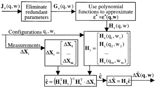
Figure 4.1 -Flow-chart of the Method to Identify Generalized Errors...52

Figure 4.2 -Joint Parameter Definition for the PPS ... 53

Figure 4.3 -Leica 3D Laser Tracking System...54

Figure 4.4 -Close-up View of the PPS Couch ... 54

Figure 4.5(a) -Measured and Residual Errors After Compensation...56

Figure 4.5(b) -Measured and Residual Errors After Compensation ... 57

Figure 4.6 -Repeatability D istribution... 58

Figure 4.7 -Measured and GEC Predicted Errors along the X Axis at NTP ... 60

Figure 4.8 -Measured and GEC Predicted Errors along the Y Axis at NTP ... 61

(8)

Figure 4.9 -Measured and GEC Predicted Errors along the Z Axis at NTP...62

Figure 4.10 -Statistics of the Compensated PPS Errors at NTP ... 63

Figure 4.11 -Schilling Titan II M anipulator ... 64

Figure 4.12 -Base Sensor Control and Error Compensation Scheme ... 65

Figure 4.13 -Nozzle Dam Experimental System...66

Figure 4.14 -Repeatability with and without BSC ... 68

Figure 4.15 -Measured and Residual Errors After Compensation...69

Figure 5.1 -Real and Ideal Positions of a Manipulator End-Effector...74

Figure 5.2 -Calibration of Elastic Errors due to an Arbitrary Force ... 75

Figure 5.3 -Stabilization of the Arm Self-M otions ... 76

Figure 5.4 -ICR Volume as a Function of the Fixture Location...80

Figure 5.5 -ICR Volume as a Function of SEC Fixture Location...81

Figure 5.6 -Measurement Configurations for an SEC Fixture at (6,0)...82

Figure 5.7 -Extrapolated and Interpolated Regions for an SEC Fixture at (6,0) ... 82

Figure 5.8 -Extrapolated and Interpolated Regions for an SEC Fixture at (10,0) ... 83

Figure 5.9 -RMS Residual Error as a Function of the Number of Measurements...85

Figure 5.10 -Experim ental System ... 86

Figure 5.11 - SEC Fixture Using Four Spheres ... 87

Figure 5.12 - SEC Fixture Using Three Rotary Joints ... 88

Figure 5.13 -SEC Fixture Using a Spherical Joint ... 89

Figure 5.14(a) -Measured and Residual Errors After Compensation...91

Figure 5.14(b) -Measured and Residual Errors After Compensation...92

Figure 6.1 -Contact Force and Wrist Force/Torque Sensor Readings...96

(9)

Figure 6.2 -Real (a) and Simulated (b) Experimental System...99

Figure 6.3 -Base Sensor Control and Contact Force Estimation Scheme ... 101

Figure 6.4 - Typical Placement Steps Using Contact Force Visualization...102

Figure B. 1 -Parameter Definitions for the PPS...124

Figure C. 1 -Side view of the Schilling Titan II...130

Figure C.2 -Top View showing the Base Force/Torque Sensor Frame...131

List of Figures 99

(10)

List of Tables

Table 3.1 - Number of Independent Generalized Errors...44

(11)

Chapter

1 Introduction

1.1 Background and Literature Review

Large robotic manipulators are needed in field, service, manufacturing and medical applications to perform high accuracy tasks. Examples are manipulators that perform decontamination tasks in nuclear sites, space manipulators such as the Special Purpose Dexterous Manipulator (SPDM) and manipulators for medical treatment (Vaillancourt et al. 1994; Flanz 1996; Hamel et al. 1997). In these applications, a large robotic system is often needed to have very fine precision while exerting substantial task forces and torques. Its accuracy specifications may be very small fractions of its workspace. Achieving such high accuracy is difficult because of the manipulator's size and its need to carry heavy payloads, as well as high joint friction. Further, many tasks, such as space applications, require systems to be lightweight, and thus structural deformation errors can be large.

A number of approaches exist for improving fine motion manipulator performance through friction compensation. Some of these require modeling of the difficult to characterize joint frictional behavior (Canudas de Wit et al. 1996; Popovic,

I1I Chapter 1: Introduction

(12)

Shimoga and Goldenberg, 1994). Some require the use of specially designed manipulators that contain complex internal joint-torque sensors (Pfeffer, Khatib and Hake, 1989). A simple, yet effective control method has been developed that is modeless and does not require internal joint sensors (Morel and Dubowsky, 1996; lagnemma et al., 1997; Morel et al., 2000). The method, called Base Sensor Control (BSC), estimates manipulator joint torques from a self-contained external six-axis force/torque sensor placed under the manipulator's base. The joint torque estimates allow for accurate joint torque control that has been shown to greatly improve repeatability of both hydraulic and electric manipulators, but not their absolute accuracy. Here repeatability is defined as how well the system returns to its original configuration after being moved to arbitrary configurations.

Even with fine repeatability, high absolute positioning accuracy is still difficult to achieve with a large manipulator. Two principal error sources create significant end-effector errors. The first is kinematic errors due to the non-ideal geometry of the links and joints of manipulators, such as errors due to machining tolerances. These errors are often called geometric errors.

The second error source that can limit the absolute accuracy of a large manipulator is the elastic errors due to the distortion of a manipulator's mechanical components under large task loads or even its own weight.

Task constraints often make it impossible to use direct end-point sensing in a closed-loop control scheme to compensate for these errors. Therefore, there is a need for model-based error identification and compensation techniques, often called robot calibration. However, classical error compensation methods cannot correct the errors in

(13)

large systems with significant elastic deformations, because they do not explicitly consider the effects of task forces and structural compliance. Methods have been developed to deal with this problem (Drouet et al. 1998; Drouet 1999), however they depend on analytical models of the manipulator structural properties that are not easy to obtain.

Considerable research has been performed in classical robot calibration without consideration of elastic deformations (Roth et al. 1986; Hollerbach 1988; Hollerbach et al. 1996; Zhuang et al. 1996). In these methods robot position accuracy is improved using compensation methods that identify a functional relationship between the joint transducer readings and the workspace position of the end-effector based on experimental calibration measurements. The process requires the identification of the manipulator generalized errors from calibration measurements. Generalized errors characterize the relative position and orientation of frames defined at the manipulator links. These errors are found from measured data and used to predict, and compensate for, the end-point errors as a function of configuration. A major component of this process is the development of manipulator error models, some of which consider the effects of manipulator joint errors, while others focus on the effects of link dimensional errors (Waldron et al. 1979; Wu 1984; Vaishnav et al. 1987; Mirman et al. 1993). Error models have been developed specifically for use in the calibration of manipulators (Broderick et al. 1988; Zhuang et al. 1992). Some researchers have studied methods to find the optimal configurations during the calibration measurements to reduce the manipulator errors by calibration (Borm et al. 1991; Zhuang et al. 1996). Solution methods for the identification of the manipulator's unknown parameters have been studied for these

(14)

model-based calibration processes (Dubowsky et al. 1975; Zhuang et al. 1993). Most calibration methods have been applied to industrial or laboratory robots, achieving good accuracy when geometric errors are dominant and elastic errors can be neglected.

In the past, calibration methods have not explicitly compensated for elastic errors due to the wrench at the end-effector. Recently in our laboratory a method to address this problem has been developed, however it requires explicit structural modeling of the system (Drouet et al. 1998; Drouet 1999). While conceptually very similar to the classical geometric problem, the combined problem is far more complex. Compensating for geometric errors requires building a model that is a function of the n (usually 6) joint variables. To compensate for a general 6 variable end-point task wrench (three end-point forces and three end-point moments) requires a model that is a function of both the joint variables and the end-point wrench variables, or a function of at least 12 variables. The number of measurements required to characterize this 12 dimensional space is far larger than required for the 6 dimensional space. The time and cost of the physical calibration measurements often dominates the calibration problem. Simple calculations suggest that a brute force identification would require several million calibration measurements.

In addition, when implementing the above methodologies, a fundamental problem inherent in robot calibration is encountered that has not been addressed in previous research. That is, in the calibration process some of the generalized errors are redundant, and thus the effects of these redundant errors are not observable in the manipulator output. These redundant error parameters must be eliminated from the error model prior to the identification process to perform calibration with improved accuracy (Hollerbach and Wampler 1996; Ikits and Hollerbach, 1997).

14

(15)

A number of coordinate system representations have been considered to model the manipulator errors. The four-parameter representations (such as the Denavit-Hartenberg representation) are attractive since they are the minimal parameter set required to locate the reference frames of the joints (Roth, Mooring and Ravani, 1987). Such representation reduces the number of error combinations to be found, however the redundant parameters are not necessarily eliminated. In addition, the Denavit-Hartenberg (D.H.) error representation does not model some of the generalized errors in the presence of parallel joints. The entire calibration can be compromised if such errors are significant. Also, the D.H. representation is ill-conditioned when neighboring joint axes are nearly parallel. Incorporating Hayati's proposed modification to the D.H. parameterization (Hayati, 1983) eliminates the ill-conditioning problem, however it has a singularity when axes are nearly perpendicular (Hollerbach, 1988). Some authors have proposed a five-parameter representation (Hsu, Everett, 1985), however this parameterization has a sensitivity problem when neighboring coordinate origins are close together (Ziegert and Datseris, 1988).

Many papers have abandoned the D.H. representation of the errors, treating the general case of two coordinate systems related by six parameters. The six-parameter representation of the errors, called generalized error model, does not have the sensitivity problems of the D.H. representation. However, it has the disadvantage of increased redundancy (Hollerbach, 1988). Numerical methods have been proposed to eliminate redundant errors (Schr6er, 1983; Everett and Suryohadiprojo, 1988; Zhuang, Roth and Hamano, 1992), however they must be formulated in a case-by-case basis (Hollerbach and Wampler, 1996). An analytical algorithm has been proposed to eliminate the

(16)

redundant errors in the D.H. error representation (Khalil, Gautier and Enguehard, 1991), however it cannot be applied to the generalized error formulation.

After choosing an appropriate identification model and eliminating the redundant error parameters it is still necessary to measure the manipulator pose as a function of the joint angles and task loads. However, most manipulator calibration techniques require expensive and/or complicated pose measuring devices, such as theodolites. Obtaining pose measurements is generally very costly and time consuming, and must be performed regularly for very high precision systems (Everett and Lin, 1988). Many pose measurement devices have been proposed. The theodolite triangulation method consists of two or more theodolites aimed at a common target on the robot wrist (Johnson, 1980). Vira and Lau used laser interferometers with steerable reflectors to measure position and orientation of a target in space (Vira and Lau, 1986). Telescoping ball bars have been used to measure contouring accuracy along a circular contour (Lau et al., 1984).

Bennett and Hollerbach defined a general class of calibration methods, called closed-loop calibration, in which constraints are imposed on the end-effector of the robot (Bennett and Hollerbach, 1991). In this method the easily-measured joint angles are adequate to calibrate the manipulator, without requiring any external metrology system. Past closed-loop methods have required the robot to move along an unsensed sliding joint at the endpoint, or constraining the end-effector to lie on a set of planes (Scheffer, 1976; Warnecke et al., 1980; Ikits and Hollerbach, 1997; Zhuang et al., 1999).

16 Chapter 1: Introduction

(17)

1.2 Objectives of this Thesis and Summary of Results

The goal of this thesis is to develop methods to substantially improve the absolute accuracy in strong powerful manipulators lacking good repeatability and having significant geometric and elastic errors - in other words, a manipulator with real characteristics. In this work, a method that compensates for the position and orientation errors caused by geometric and elastic errors in such large manipulators is presented. The method, called Geometric and Elastic Error Compensation (GEC), explicitly considers the task load dependency of the errors, modeling both deformation and more classical geometric errors in a unified manner. A set of experimentally measured positions and orientations of the robot end-effector and measurements of the payload wrench are used to calculate the robot generalized errors without using an explicit manipulator elastic model (Meggiolaro, Mavroidis and Dubowsky, 1998). Generalized errors are those parameters that characterize the relative position and orientation of frames defined at the manipulator links. They are determined from measured data as a function of the system configuration and the task wrench. Knowing these generalized errors, the manipulator end-effector errors are compensated at any configuration. In the GEC method each generalized error parameter can be represented as a function of only a few of the system variables. As a result, the number of measurements required to characterize the system is dramatically smaller than might be expected (Meggiolaro, Dubowsky and Mavroidis, 2000). The GEC method is applied in concert with a previously developed concept called Base Sensor Control (BSC), which ensures good repeatability by compensating for joint friction. The combined methods do not require joint velocity or acceleration measurements, a model of the actuators or friction, or the

(18)

knowledge of manipulator mass parameters or link stiffnesses, yet they are able to improve substantially its absolute positioning accuracy (Meggiolaro, Jaffe and Dubowsky, 1999).

As discussed before, to improve calibration accuracy, redundant error parameters must be eliminated from the error model prior to the identification process. In this thesis, analytical expressions and physical interpretation of all redundant error parameters are developed for any serial link manipulator. These expressions allow for systematic calibration with improved accuracy of any serial link manipulator (Meggiolaro and Dubowsky, 2000).

After choosing an appropriate identification model and eliminating its redundant error parameters, it is still necessary to measure the manipulator pose at different configurations. However, most manipulator calibration techniques require expensive and/or complicated pose measuring devices, such as theodolites. This thesis presents a calibration method, called Single Endpoint Contact (SEC) calibration, where the manipulator endpoint is constrained to a single contact point while the robot executes

self-motions. From the easily-measured joint angle readings and an identification model, the manipulator is calibrated (Meggiolaro, Scriffignano and Dubowsky, 2000).

1.3 Applications

Two real applications are studied in this thesis. They are a patient positioning system for radiation therapy and a maintenance task in the nuclear power industry.

Chapter 1: Introduction 18

(19)

1.3.1 Patient Positioning System

The robotic Patient Positioning System (PPS) at the proton therapy research facility constructed at the Massachusetts General Hospital (MGH), the Northeast Proton Therapy Center (NPTC), is an example of a large medical manipulator (Flanz et al. 1995; Flanz et al. 1996). The PPS places a patient in a high energy proton beam delivered from a proton nozzle carried by a rotating gantry structure (see Figure 1.1). The PPS is a six degree-of-freedom manipulator that covers a large workspace of more than 4m radius while carrying patients weighing as much as 300 lbs (see Figure 1.2). Patients are immobilized on a "couch" attached to the PPS end-effector. The PPS, combined with the rotating gantry that carries the proton beam, enables the beam to enter the patient from any direction, while avoiding the gantry structure. Hence programmable flexibility offered by robotic technology is needed.

Figure 1.1 -The PPS and the Gantry [Ref. Flanz, 1996]

Chapter]: Introduction 19

(20)

Longitudinal _{6 Axis Force/} _Treatment

Axis _{Torque Sensor} _Volume

Couch

Vertical Axis

Roll/Pitch Drive Rotary Drive

Lateral Axis

Figure 1.2 -_{The Patient Positioning System [Ref. Flanz, 1996]}

The required absolute positioning accuracy of the PPS is ±0.5 mm. This accuracy is critical as larger errors may be dangerous to the patient (Rabinowitz 1985). The required accuracy is roughly 104 _{of the nominal dimension of the system workspace.}

This is a greater relative accuracy than most industrial manipulators. In addition, FEM studies and experimental results show that with a changing payload (between 1 and 300 pounds) and changing configuration the end-effector errors due to elastic deformations and geometric errors are of the order of 6-8 mm. Hence the accuracy is 12 to 16 times the system specification (Mavroidis et al. 1997). However, since the repeatability error of the PPS, defined here as how well the system returns to certain arbitrary configurations, is less than 0.15mm, it is a good candidate for a model based error correction method.

(21)

The GEC calibration method was applied to the PPS with a force/torque sensor built into the system to measure the wrench applied by the patient's weight. It was found that using only 450 calibration measurements the end-point errors could be reduced to well within the required specification. In fact, experimental results show that the maximum error is reduced by a factor of 18.

1.3.2 Nozzle Dam Placement

Another application of large robotic manipulators is in the nuclear power industry. The dangerous task of steam generator maintenance is currently performed by workers, who are referred to as "jumpers." Once a year, each nuclear reactor is shutdown for a month to swap old fuel rods in the reactor core with new ones (Figure 1.3 shows a graphical overview of the process for a Westinghouse type F steam generator). At the same time the fuel cells are replenished, the U-tubes in the steam generator must be inspected for damage. In order for workers to enter the steam generator, the water in the reactor core must be prevented from entering the steam generator's water chamber. This is achieved by covering the two large portals, one meter in diameter, that connect the hot and cold pipes to the steam generator (Cho, 1997). Each portal has a nozzle ring into which a device referred to as a nozzle dam is inserted with a tolerance of approximately 1mm. The nozzle dam is installed in two phases, the first of which is fitting the nozzle dam side plate in the nozzle ring (Figure 1.4a), and then the nozzle dam center plate is placed within the side plate (Figure 1.4b). This provides the necessary seal to prevent water leakage, thereby allowing workers to enter the steam generator and inspect the U-tubes.

(22)

Recor RefueliinR vessel Machine CoIer . LOOP CONCENSER FEOWATER SYSTEM SEAWATER / FSEAWATER 0 m Steamn Geneator NOZZLE DAM V/

H(;Leg Nuzzle Darn Placement

Provides Simutancous

Operation of Refueling

ndS/C U-Ttbe lnspeaaion (ECT)&

Cdld Lex Maintenance

Figure 1.3 -Nuclear Reactor [Ref. Cho, 1997]

Nozzle Dam Center Plate

Side Plate

(a) (b)

Figure 1.4 -Simulated Robotic Nozzle Dam Task

Installing one nozzle dam requires hours of manual labor during which time the workers are exposed to high doses of residual radiation. Jumpers can only remain in the steam generator chamber for three minutes before receiving their maximum acceptable

(23)

yearly radiation dosage. At this point, the worker leaves the chamber through the 0.8 m diameter access portal and another worker enters to resume the task (Zezza, 1985). The manpower and time required to complete this task, as well as the health risks imposed on the workers, make this task well suited to investigations in automating the process. Recent attempts to place the nozzle dam with a manipulator have taken very long because of the combination of poor teleoperator visibility and lack of manipulator accuracy. Successful completion of the task with a manipulator would eliminate radiation exposure as well as save money by reducing the time required to place the nozzle dam. For each hour that the reactor is off line, $40,000 in potential revenues is lost. The key to achieving this task is improving manipulator accuracy as well as the operator interface. The typical repeatability of manipulators capable of handling the required load, such as the Schilling Titan II manipulator, is in the range of 10 to 20 mm. The absolute accuracy can be several times these amounts. The automation of this task would require absolute

accuracy of only a few millimeters.

Also, contact force information between the manipulator end-effector and the environment is fundamental for teleoperated placement tasks with small tolerances. However, a wrist force/torque sensor alone provides limited information to locate the contact point. In the case where there is only one contact point with the environment and where the contact torque is zero, it is possible to calculate the contact information required for control. This can be obtained from wrist force/torque information combined with knowledge of the geometry of the manipulator end-effector. A method is developed to estimate the contact forces between the manipulator end-effector and the environment

Chapter 1: Introduction 23

(24)

from wrist sensor and task geometry, and graphically displays this contact force information to a teleoperator (Meggiolaro, Jaffe, lagnemma and Dubowsky, 1999).

In addition, a virtual viewing system based on 3-D kinematic models is developed to perform the nozzle dam task. The system contains 3-D kinematic models of the manipulator and the workspace, reflecting the actual system configuration. The interface provides improved operator visibility by allowing virtual viewing of physically obscured regions using virtual cameras. The virtual cameras also allow for magnifying the mating edges in order to aid in teleoperated insertion tasks. The virtual viewing system is combined with real-time contact force measurements to improve teleoperation. Laboratory experiments show that successful nozzle dam placements could be performed using the combined GEC/BSC techniques and the visualization system with a

conventional Schilling hydraulic manipulator.

1.4 Outline of this Thesis

This thesis is divided into seven chapters. This chapter serves as an introduction and overview of the work. Chapter 2 reviews the Base Sensor Control method as applied to the fine-motion positioning problem, and presents the generalized error formulation applied to classical manipulator calibration.

Chapter 3 presents a general analytical method to eliminate the redundant error parameters in robot calibration. Simulation results are presented for a PUMA 560 and for an Adept SCARA manipulator.

(25)

Chapter 4 describes the GEC (Geometric and Elastic Error Compensation) theory and shows experimental results for the calibration of the Patient Positioning System and of a Schilling Titan II manipulator used in the nozzle dam placement task.

Chapter 5 investigates the SEC (Single Endpoint Contact) calibration method, where the robot endpoint is constrained to a single contact point. Optimization of the SEC fixture location is discussed. Simulations and experimental results are presented for a Schilling Titan II manipulator.

Chapter 6 explores a method to obtain contact force information between the manipulator end-effector and the environment. This method is applied to a virtual environment teleoperator interface developed for the nozzle dam placement task. This system is then integrated with control hardware to provide a comprehensive teleoperation package.

Chapter 7 summarizes the conclusions regarding the integration of the above methodologies. Finally, suggestions for further work are presented.

The appendices to this thesis give detailed information on specific topics related to the practical implementation of the work presented. Appendix A provides the proof of the linear combination expressions of the columns of the Identification Jacobian matrix. These expressions are used to eliminate the redundant parameters from the error model in robot calibration. Appendix B provides a kinematic description of the Patient Positioning System, including the associated error matrices. Appendix C provides the error matrices for the Schilling Titan II manipulator.

(26)

Chapter

2 Analytical Background

2.1 Introduction

This chapter reviews the analytical background for Base Sensor Control and classical calibration techniques. Section 2.2 reviews the theoretical framework for the BSC method, and discusses important simplifications that can be made for the fine-motion case. Section 2.3 presents the generalized error formulation applied to classical robot calibration.

2.2 Base Sensor Control (BSC)

The following is a brief review of the basis for BSC (Base Sensor Control) based on (Morel et al., 2000), where the complete development is presented. A simplified version of the algorithm sufficient and effective for fine-motion control is formulated in (lagnemma, 1997).

BSC has been developed to compensate for nonlinear joint characteristics in robotic manipulators, such as high joint friction, to improve system repeatability. BSC estimates manipulator joint torques from a self-contained external six-axis force/torque

(27)

sensor placed under the manipulator's base. The joint torque estimates allow for accurate joint torque control that has been shown to greatly improve repeatability of both

hydraulic and electric manipulators.

As shown in Figure 2.1, the wrench, Wb, exerted by the manipulator on its base sensor can be expressed as the sum of three components:

Wb = Wg + Wd + We (2.1)

where Wg is the component due to gravity, Wd is caused by manipulator motion, and We is the wrench exerted by the payload or task on the end-effector. Note that joint friction does not appear in the measured base sensor wrench. In the fine-motion case, it is assumed that the gravity wrench is essentially constant, and this wrench can be approximated by the initial value measured by the base sensor. Hence, the complexity of computing the gravitational wrench, such as identification of link weights and a static manipulator model, is eliminated. Under this assumption, the Newton Euler equations of the first i links are:

WO, _{= -Wb}

Wl) = WO ₁- Wd,

Wi-A+1 = W-l-- - Wd. (2.2)

We = Wn_-. - Wd.

where Wie+ is the wrench exerted by link i on link i+1, and Wd, is the dynamic wrench for link i.

Chapter 2: Analytical Background 27

(28)

Wd Wee W 1 Wrist Force/ Torque Sensor _Wd, W Wb W + W + We 91 Base Force/ Torque Sensor Figure 2.1 -_{External and Dynamic Wrenches [Ref. Morel et al., 1996]}

For fine tasks it is assumed that the manipulator moves very slowly so that Wd

can be neglected. Therefore, for slow, fine motions, only the measured wrench at the base is used to estimate the torque in joint i+1. The estimated torque in joint i+1 is obtained by projecting the moment vector at the origin O of the ith reference frame along the joint axis zi:

ri+I = -ziT. Wb (2.3)

The value of 'ri,1 depends only on the robot's kinematic parameters, joint angles

and base sensor measurements.

With estimates of the joint torque, it is possible to perform high performance torque control that can greatly reduce the effects of joint friction and nonlinearities. This results in greatly improved repeatability. Figure 2.2 shows BSC schematically.

Chapter 2: Analytical Background 28₂₈

(29)

A Virtually Frictionless Robot Base Force/Torque Desired Sensor Position _Torque Estimation Motor + -Current Position esedTorque

Control Toqe +Control

Joint Position Sensors

Figure 2.2 -BSC Control Loop [Ref. Morel et al., 1996]

However, the BSC method will not compensate for sources of random repeatability errors, such as limited encoder resolution. In addition, a manipulator with good repeatability may not have fine absolute position accuracy. After improving the system repeatability using BSC, a model-based error correction method can be applied to reduce the absolute accuracy errors. The next section presents a classical formulation for manipulator calibration.

2.3 Classical Manipulator Calibration

There are many possible sources of errors in a manipulator. These errors are referred to as "physical errors," to distinguish them from the generalized errors defined in Chapter 1. In most cases, while the actual physical errors are relatively small, their effect at the end-effector is large. The main sources of physical errors in a manipulator are: * Mechanical system errors: These errors result from machining and assembly

tolerances of the manipulator's mechanical components.

29 Chapter 2: Analytical Background

(30)

" Deflections: Elastic deformation of the manipulator's members under task loads and

gravity can result in large end-effector errors, especially in long reach manipulator systems.

" Measurement and Control: Measurement, actuator, and control errors that occur in the control systems will create end-effector positioning errors. The resolution of encoders and stepper motors are examples of this type of error.

" Joint errors: These errors include bearing run-out in rotating joints, rail curvature in linear joints, and backlash in manipulator joints and actuator transmissions.

Further, errors can be distinguished into "repeatable" and "random" errors (Slocum, 1992). Repeatable errors are those whose numerical value and sign are constant for a given manipulator configuration and task load. An example of a repeatable error is an assembly error. Random errors are errors whose numerical value or sign changes unpredictably. An example of a random error is the error that occurs due to backlash of an actuator gear train. Classical kinematic calibration and correction can only deal with repeatable errors. It will be shown experimentally in Chapter 4 that repeatable errors dominate in the performance of the PPS and of the Schilling manipulator.

To describe the kinematics of a manipulator, Denavit-Hartenberg reference frames are defined at the manipulator base, end-effector, and at each manipulator joint (Craig, 1989). The position and orientation of a reference frame Fi with respect to the previous reference frame Fi- is defined with a 4x4 matrix Ai that has the general form:

A1=[Ri T] (2.4)

10 1](.4

(31)

The Ri term is a 3x3 orientation matrix composed of the direction cosines of frame Fi with respect to frame Fi-1, and Ti is a 3x1 vector of the coordinates of center Oi of frame Fi in Fi-1, see Figure 2.3. The elements of matrices Ai depend on the geometric parameters of the manipulator and the manipulator joint variables q.

Frame F ideal

A 1 E.

1 No errors 1

Frame F real _ii Frame F.real

1

o ideal With errors

Otrea

o

_i-Ireal

Figure 2.3 -Frame Translation and Rotation Due to Errors for ith Link

Physical errors cause the geometric parameters of a manipulator to be different from their ideal values. As a result, the frames defined at the manipulator joints are slightly displaced from their expected, ideal locations, creating significant end-effector

real

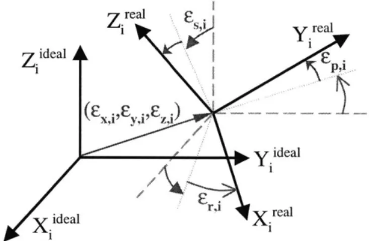
errors. The position and orientation of a frame Fa with respect to its ideal location Fiideal is represented by a 4x4 homogeneous matrix Ei, see Figure 2.3. The translational part of matrix Ei is composed of the 3 coordinates Ex,i, Ey,i and Ez,i of point Oireal in Fiideal (along the X, Y and Z axes respectively, defined using the Denavit-Hartenberg representation), see Figure 2.4. The rotational part of matrix Ei is the result of the product of three consecutive rotations cs,i, Er,i, -p,i around the Y, Z and X axes respectively

real ideal

(also shown in Figure 2.4). These are the Euler angles of Fa with respect to Fii . The subscripts s, r, and p represent spin (yaw), roll, and pitch, respectively. The 6 parameters

Exi, E'yi, £zi, Esj, Er,i and epi are called generalized error parameters, which can be a

(32)

function of the system geometry and joint variables. For an n degree of freedom manipulator, there are 6(n+1) generalized errors which can be written in the form of a

6(n+1) x l _{vector E = [EX,O,..., Exi, Eyji EzJ, EsJ , Er,i, Epi,..., Ep,n] , with i ranging from 0 to n,} assuming that both the manipulator and the location of its base are being calibrated. If the manipulator is being calibrated with respect to its own base, then the error matrix EO (which models the errors of the base location) is eliminated, reducing the number of generalized errors to 6n. The generalized errors that depend on the system geometry, the system task loads and the system joint variables can be calculated from the physical errors link by link. Note that system weight effects can be included in the model as a simple function of joint variables.

Zi rea real

Z ideal

y ideal

X iideal Xira

Figure 2.4 -Translational and Rotational Generalized Errors for ith Link

With generalized errors the manipulator loop closure equation takes the form: ALC(q,e,s) = E0A1E1A2E2... AnEn (2.5)

where ALC is a 4x4 homogeneous matrix of the form of Equation (2.4) that describes the position and orientation of the end-effector frame with respect to the inertial reference frame as a function of the configuration parameters q, the vector of the generalized errors

32

(33)

E, and the vector of the structural parameters s. The translational components of the matrix ALc and the three angles of its rotational components are the six coordinates of the end-effector position and orientation vector Xreal.

The end-effector position and orientation error AX is defined as the 6x1 vector that represents the difference between the real position and orientation of the end-effector and the ideal one:

AX = Xreal - Xideal (2.6)

where Xreal and Xideal are the 6x1 vectors composed of the three positions and three

orientations of the end-effector reference frame in the inertial reference system for the real and ideal cases, respectively.

Since the generalized errors are small, AX can be calculated by the following linear equation in E:

AX = Je E (2.7)

where Je is the 6x6(n+1) Jacobian matrix of the end-effector error AX with respect to the elements of the generalized error vector E, also known as Identification Jacobian matrix (Zhuang et al. 1999). As with the generalized errors, Je depends on the system

configuration, geometry and task loads.

If the generalized errors, E, can be found from calibration measurements, then the

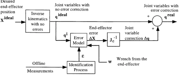
correct end-effector position and orientation error can be calculated using Equation (2.7) and be compensated. Figure 2.5 shows schematically an error compensation algorithm

based on Equation (2.7). The method to obtain E from experimental measurements is explained below.

(34)

Desired end-effector position Xideal

Joint variables with Joint variables with

no error correction error correction

Inverse qideal ₊ _qreal

kinematics + q

with no

errors End-effector Joint +

qi error variable

Error AX -1 correction Aq

Model J

Wrench from the

Offline Identification end-effector

Measurements Process

Figure 2.5 - Error Compensation Scheme

To calculate the generalized errors , it is assumed that some components of vector AX can be measured at a finite number of different manipulator configurations. However, since position coordinates are much easier to measure in practice than orientations, in many cases only the three position coordinates of AX are measured.

Assuming that all 6 components of AX can be measured, for an n degree of freedom manipulator, 6(n+1) generalized errors e can be calculated by measuring AX at

m different configurations, defined as qi, q2,..., qm, then writing Equation (2.7) m times:

AX,

HJ(q)

~ (2.8

A

e(qi)

AX2 Je(2) _IFj.

A, =

I

... | | ...

I

,-E(2.8)

LAXmJ LJe(q.)j

where AXt is the m x 1 vector formed by all measured vectors AX at m different configurations and Jt is the 6m x 6(n+l) matrix formed by the m Identification Jacobian matrices Je at m configurations, called here Total Identification Jacobian. To reduce the effects of measurement noise, the number of measurements m is, in general, much larger than n.

(35)

If the generalized errors E are constant, then a unique least-squares estimate $ can be calculated by:

s=(JTJ,)J T -AX, (2.9)

However, if the Identification Jacobian matrix Je(qi) contains linearly dependent columns, Equation (2.9) will produce estimates with poor accuracy due to poor matrix conditioning (Hollerbach et al. 1996). This occurs when there is redundancy in the error model, in which case it is not possible to distinguish the error contributed by each generalized error component. Conventional calibration methods also cannot be successfully applied when some of the generalized errors depend on the manipulator configuration q or the end-effector wrench w, namely E(q,w), such as when elastic deflections that depend on the configuration and applied forces at the end-effector are significant. Chapters 3 and 4 present respectively methods for finding the generalized errors (E) for the case where there is a singular Identification Jacobian matrix and where there are significant elastic deformations combined with conventional geometric errors.

2.4 Summary and Conclusions

This chapter presented the theoretical framework for the BSC method, and a simplified form of the algorithm was formulated for the fine-motion case. A generalized error formulation was presented for classical manipulator calibration, which can be used to identify the system geometric errors. However, classical calibration methods do not explicitly compensate for elastic errors due to the wrench at the end-effector. In addition, redundant error parameters must be eliminated from the error model prior to the identification process to perform calibration with improved accuracy. Chapters 3 and 4

(36)

present an analytical method to eliminate the redundant parameters, and introduce a calibration method that identifies both geometric and elastic deformation errors.

Chapter 2. Analytical Background 36

(37)

Chapter

3 Elimination of Redundant Error Parameters

3.1 Introduction

This chapter presents a general analytical method to eliminate redundant error parameters in robot calibration. Section 3.2 presents analytical expressions and physical interpretation of the linear combinations of generalized errors. Section 3.3 contains simulation results for a PUMA 560 and an Adept SCARA manipulator, showing the number of identifiable error parameters in each case and comparing the analytical formulation to ad-hoc methods.

3.2 Eliminating Redundant Errors

In robot calibration, redundant errors must be eliminated from the error model prior to the identification process. This is usually done in an ad-hoc or numerical manner by reducing the columns of the Identification Jacobian matrix Je to a linearly independent set (Hollerbach, 1988). Here, an analytical method is presented to eliminate the redundant parameters. Section 3.2.1 presents the linear combinations of the columns of the Identification Jacobian matrix and the method to eliminate the redundant errors to obtain the non-singular Identification Jacobian matrix. Section 3.2.2 discusses physical

(38)

interpretations of the linear combinations. Section 3.2.3 presents additional linear combinations introduced when only the end-effector position is measured. Section 3.2.4 shows the number of independent error parameters for a general serial link manipulator. Section 3.2.5 extends the results obtained using the six-parameter representation to the Denavit-Hartenberg error parameterization. It also shows that the D.H. representation of errors does not model some of the generalized errors in the presence of parallel joints, which can adversely affect the identification process.

3.2.1 Linear Combinations of the Identification Jacobian matrix

In this section, the linear combinations of the columns of the Identification Jacobian matrix Je are presented. The six-parameter representation is used to define the errors, and the linear combination coefficients are expressed through the robot's D.H.

parameters. Defining

Jx,

1, Jyj, Jzi, Jsi, Jri and

Jp,i

as the columns of

J,

associated with the

generalized error components Ex,i, Ey,i, EzJi EsJ9 E-r,i and Ep,i respectively (i between 0 and n),

Equation (2.7) can be rewritten as

AX = [,.J4I yJ I,'I S, JOI J J , .,]

[EX,... E ,-J E Y, EJ -,i , 01 E P, . .. , E p] T(3.1)

For each link i, between 1 and n, the following linear combinations are always valid (see Appendix A for proof):

Jz~i-1) =sin cc JJ + o ij Z'i _(3.2)

Jr,(i-) _{aa cosiJYJ -a sinxiJz, +sinxiJs}

1 +coscJrO (3.3)

(39)

where the manipulator parameters are defined using the D.H. representation: link lengths ai, joint offsets di, joint angles

ei,

and skew angles ci. If joint i is prismatic, then additional combinations of the columns of Je are found:

J x,(i-1) JX,i _(3.4)

Jy,(i-1) _{= cos aiJ yj - sin aciJz'i}

(3.5)

The linear combinations shown above are always present, independently of the values of ai and

oi,

even for degenerate cases (such as ai=O). As shown in Appendix A, if the full pose of the end-effector (both position and orientation) is measured, then Equations (3.2-3.5) are the only linear combinations for link i.

To obtain the non-singular Identification Jacobian matrix, called here Ge, columns

Jz,(i-I) and Jr,(i-1) must be eliminated from the matrix J, for all values of i between 1 and n.

If joint i is prismatic, then columns Jx,(i-1) and Jy,(i_1) must also be eliminated. For an n

DOF manipulator with r rotary joints and p (p equal to n-r) prismatic joints, a total of

2r+4p columns are eliminated from the Identification Jacobian Je to form its submatrix

Ge. This means that 2r+4p generalized errors cannot be obtained by measuring the end-effector pose.

By definition, the dependent error parameters eliminated from E do not affect the end-effector error, resulting in the identity

AX = Je E = Ge E* (3.6)

Using the above identity and the linear combinations of the columns of J, from Equations (3.2-3.5), it is possible to obtain all relationships between the generalized error set E and

(40)

its independent subset, E* (see Appendix A). If joint i is revolute (i between 1 and n),

then the generalized errors EZ,(i1) and r,(i-1) are eliminated, and its values are incorporated

into the independent error parameters E*yi, e* zj, e s,i and E r,i:

si *c+r~1 a COWOC

E i +Ezi- sin +Er(i-1) - i ci

Ez'= Ez,i + Ez,(i-1 cos(X - Eri-1 -ai sin cci

C= ESJ + Er,(i-l sin oi

6ri=ErJi + Eri-l) C c i

(.7

If joint i is prismatic, then the translational errors Exi-1) and ey,(i_1) are eliminated,

and its values are incorporated into the independent error parameters e*x,i, E*y,i and E*z,i- In this case, Equation (3.7) becomes:

F + +E

y i E +i y ,(i-1) + z,(i-1) sin i + Er,(i-) ai cos ci z'i _ez'i- E_1) sin cx + Esi-g cosOc - Ei- ai sin oi

z,(-1 ii1

sin-1 aasn c

ssE + (_1 sin cc

r r,i + r,(i-1) cos _(3.8)

If the vector &* containing the independent errors is constant, then the matrix _Ge

can be used to replace Je in Equation (2.7), and Equation (2.9) is applied to calculate the estimate of the independent generalized errors E*, completing the identification process. However, if non-geometric factors are considered (e.g. link compliance, gear eccentricity), then it is necessary to further model the parameters of E* as a function of the system configuration prior to the identification process. This situation will be discussed in Chapter 4.

(41)

3.2.2 Physical Interpretation of the Linear Combinations

In this section the physical interpretation of Equations (3.2-3.5) is presented. Each equation associates a generalized error from link i-1 with a combination of errors from link i that result in end-effector errors of the same magnitude and direction. Since it is not possible to distinguish the amount of error contributed by each generalized error, the errors associated with link i-I are indistinguishable.

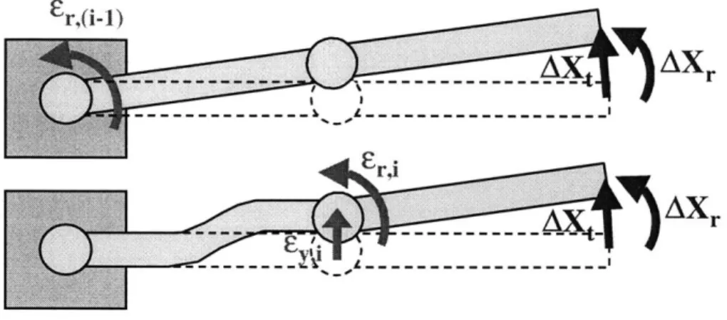
Equation (3.2) reflects the fact that the translational error along the Z-axis of frame i- 1 has the same effect as a combination of the translational errors along the Y and Z axes of frame i (see Figure 3.1). This relation is easily explained by the fact that the skew angle xi between the axes of joints i-1 and i is constant.

Figure 3.1 -Linear Combination of Translational Generalized Errors

Equation (3.3) states that the rotational error along the Z-axis of frame i-I has the same effect as a combination of the rotational and translational errors along the Y and Z axes of frame i. For simplicity, a planar manipulator is used to explain this combination (see Figure 3.2). The top figure shows the end-effector translational and rotational errors AXt and AXr caused by the rotational generalized error Eri1 of frame i-1. The bottom figure shows that the same end-effector errors can be reproduced by a specific combination of the translational error Eyi and the rotational error Er,i of frame i. To obtain

(42)

the same end-effector errors in this case, it is required that Eyi = Er,(i-1) - ai and Er,i = Er,(i-1)

(see the relationship between E* and , in Appendix A).

--- -- -- - -- - - . AXr

Fr,i

X

~)AXr

--- 1

---Figure 3.2 - Error Combinations Resulting in Same End-Effector Errors

If joint i is prismatic, then Equations (3.4) and (3.5) are also valid. These combinations simply state that the effects of the generalized errors along the X and Y

axes of frame i-I can always be reproduced by a combination of the three translational

generalized errors of frame i (see Figure 3.3). This is always true for prismatic joints, since such joints only move along the Z-axis of frame i-1 (using the D.H. frame definition).

FiEr

Figure 3.3 - Linear Combinations of Generalized Errors in Prismatic Joints

(43)

3.2.3 Partial Measurement of End-Effector Pose

The linear combinations of the columns of the Identification Jacobian matrix Je shown in Equations (3.2-3.5) are obtained when both position and orientation of the end-effector are considered. In the case where only the end-end-effector position is measured, its orientation can take any value, resulting in additional linear combinations. In this case, the three last columns of Je are zero vectors (see Appendix A):

Js,n : Jr,n Jp,n 0 (3.9)

Equation (3.9) means, as expected, that the three rotational errors of the end-effector frame Es,n, Fr,n and Ep,n do not influence the end-effector position (they only affect the orientation, which is not being measured). As a result, these generalized errors are not obtainable.

If the last joint is prismatic, then no further linear combinations are found. However, if the last joint is revolute and its link length a,, is zero, then three more linear combinations are present (see Appendix A):

Js,(n-1) dn Jx,(n-1) (3.10)

Jp,(n-1) - dn Jy,(n-1) (3.11)

Jr,(n-1) 0 (3.12)

meaning that the effects of Es,(n-1) and Ep,(n-1) cannot be distinguished from the ones caused

by Ex,(n-1) and Ey,(n-1), and also the generalized error Er,(n-1) is not obtainable. If both link length an and joint offset dn are zero, then the origin of frames n-I and n coincide at the end-effector position. In this case, Equations (3.9-3.12) can be recursively applied to frames n-I, n-2, and so on, as long as the origin of these frames all lie at the end-effector position. See Appendix A for more details.

(44)

3.2.4 Number of Independent Generalized Errors

As a corollary of Equations (3.2-3.12), the number of independent generalized errors for a generic serial link manipulator can be calculated. Upper bounds of this number have been presented in the literature (Roth, Mooring and Ravani, 1987; Zhuang, Roth and Hamano, 1992), but not its exact value. Table 3.1 shows the number of generalized errors, the number of linear dependencies, and the number of independent generalized errors for both robot calibration (without modeling its base frame errors) and robot plus base location calibration.

Table 3.1 - Number of Independent Generalized Errors

Robot+Base Calibration Robot Calibration

# generalized errors 6(n+ 1) 6n

# linear dependencies 2r + 4p + k 2r' + 4p' + k

# independent errors 6(n+1) - (2r + 4p + k) 6n - (2r' + 4p' + k)

where

n: # of joints in the manipulator

r; r' : # of revolute joints including/excluding joint 1

p ; p': # of prismatic joints including/excluding joint 1 0 if measuring end -effector position and orientation

3 if only measuring end -effector position and either the last joint is prismatic or an 0 3+2q if only measuring end -effector position, the last q joints are revolute,and

an-q+1 an-q+2a n-q+3 an and dn-q+2 dn-q+3 n =0