A three-dimensional model study of long-term mid-high latitude lower stratosphere ozone changes

HAL Id: hal-00295320

https://hal.archives-ouvertes.fr/hal-00295320

Submitted on 27 Aug 2003

HAL is a multi-disciplinary open access

archive for the deposit and dissemination of

sci-entific research documents, whether they are

pub-lished or not. The documents may come from

teaching and research institutions in France or

abroad, or from public or private research centers.

L’archive ouverte pluridisciplinaire HAL, est

destinée au dépôt et à la diffusion de documents

scientifiques de niveau recherche, publiés ou non,

émanant des établissements d’enseignement et de

recherche français ou étrangers, des laboratoires

publics ou privés.

latitude lower stratosphere ozone changes

M. P. Chipperfield

To cite this version:

M. P. Chipperfield. A three-dimensional model study of long-term mid-high latitude lower

strato-sphere ozone changes. Atmospheric Chemistry and Physics, European Geosciences Union, 2003, 3 (4),

pp.1253-1265. �hal-00295320�

www.atmos-chem-phys.org/acp/3/1253/

Chemistry

and Physics

A three-dimensional model study of long-term mid-high latitude

lower stratosphere ozone changes

M. P. Chipperfield

School of the Environment, University of Leeds, Leeds, UK

Received: 8 January 2003 – Published in Atmos. Chem. Phys. Discuss.: 25 February 2003 Revised: 1 August 2003 – Accepted: 4 August 2003 – Published: 27 August 2003

Abstract. We have used a 3D off-line chemical transport

model (CTM) to study the causes of the observed changes in ozone in the mid-high latitude lower stratosphere from 1979–1998. The model was forced by European Centre for Medium Range Weather Forecasts (ECMWF) analyses and contains a detailed chemistry scheme. A series of model runs were performed at a horizontal resolution of 7.5◦×7.5◦and covered the domain from about 12 km to 30 km. The basic model performs well in reproducing the decadal evolution of the springtime depletion of ozone in the northern hemi-sphere (NH) and southern hemihemi-sphere (SH) high latitudes in the 1980s and early 1990s. After about 1994 the modelled in-terannual variability does not match the observations as well, which is probably due in part to changes in the operational ECMWF analyses – which places limits on using this dataset to diagnose dynamical trends. For mid-latitudes (35◦–60◦) the basic model reproduces the observed column ozone de-creases from 1980 until the early 1990s. Model experiments show that the halogen trends appear to dominate this mod-elled decrease and of this around 30–50% is due to high-latitude processing on polar stratospheric clouds (PSCs). Dy-namically induced ozone variations in the model correlate with observations over the timescale of a few years. Large discrepancies between the modelled and observed variations in the mid 1980s and mid 1990s can be largely resolved by assuming that the 11-year solar cycle (not explicitly included in the 3D model) causes a 2% (min-max) change in mid-latitude column ozone.

1 Introduction

The determination of the cause of the observed downward trend in ozone at mid-latitudes has been a focus of strato-spheric research over the past decade (e.g. WMO, 1999).

De-Correspondence to: M. P. Chipperfield

(martyn@env.leeds.ac.uk)

spite the identification of many possible contributing chem-ical and dynamchem-ical processes, and a range of modelling and observational studies, a quantitative attribution of the trend has not yet been obtained. Such quantitative attribution de-pends greatly on comprehensive model simulations which can account for all known processes. Due to the limitations of different types of model, such simulations have not yet been performed. In this paper we apply for the first time a detailed full chemistry 3D stratospheric chemical transport model to the study of decadal mid-latitude ozone changes.

In contrast to the large ozone loss observed in the Antarc-tic spring, and in the ArcAntarc-tic during recent cold winters, ozone depletion at mid-latitudes is much smaller. At northern hemi-sphere (NH) mid-latitudes (35◦_N–60◦_{N) the annual} aver-aged ozone was observed to decrease by about 2% from 1979 values during the 1980s. Additional larger losses occurred during 1992–1993, following the eruption of Mt. Pinatubo in 1991. Subsequently, during the mid-late 1990s ozone levels increased and by the late 1990s the mean ozone column was around 3–4% below the 1979 values. In contrast, the mean ozone column in the southern hemisphere (SH) mid-latitudes (35◦–60◦S) exhibited a relatively steady decline from 1979 without a large decrease after the Mt. Pinatubo eruption. By the late 1990s mean SH mid-latitude columns were about 5% less than 1979. This hemispheric asymmetry, and the appar-ent lack of a Pinatubo signal in the SH, has not yet been ex-plained.

Different processes have been proposed to explain the ob-served mid-latitude trends. Chemical processes are essen-tially related to halogen (chlorine/bromine) trends which are known to be responsible for the large seasonal depletion in the polar regions. At mid-latitudes halogen chemistry may deplete ozone by:

– The export of O3-poor air from the polar vortex at the

end of spring (“dilution”).

– The export of activated air during the winter/spring from

– The “in-situ” activation of chlorine at mid-latitudes on

cold liquid aerosol particles.

(Note that the chemical depletion of ozone around 40 km in the upper stratosphere by chlorine makes only a relatively small contribution to the column (see Chipperfield and Ran-del, 2003). More recently other “dynamical” process have been suggested as contributing to the trend. These processes include

– Changes in wave-driving. – Trends in tropopause height.

It is likely that the observed trend has contributions from more than one of these processes, and the relative contribu-tions vary between the hemispheres and possibly interannu-ally.

Early studies which addressed the role of halogen trends in mid-latitude ozone used two-dimensional (2D) latitude-height models (e.g. Solomon et al., 1996, 1998; Jackman et al., 1996; Callis et al., 1997). These studies, and subsequent updates (e.g. Portmann et al., 1999), have suggested that in-creasing halogens are likely to have been a major cause of the decreasing trend observed in the NH. Furthermore, pro-cessing on mid-latitude liquid aerosol is a key step in acti-vating the chlorine and causing ozone depletion. In partic-ular, a strong argument for the link between halogen activa-tion on mid-latitude aerosol and ozone loss came from the 2D models’ ability to simulate the enhanced loss during the 1992–1993 period. Unfortunately, the published 2D model results have focused on the NH mid-latitudes and there is no information about the modelled trends in the SH. Also, as po-lar processes are a potentially important contributor to mid-latitude changes the different extent of vortex depletion and meteorological conditions in the south provide an important test of models.

Three-dimensional (3D) models are now being applied to multiannual simulations of the stratosphere (e.g. Chipper-field, 1999; Rummukainen et al., 1999; Egorova et al., 2001). These models have some advantages over two-dimensional models. The models are better able to represent the dynam-ics of the polar vortices and hence the associated chemical depletion. Also, when these models are forced by meteoro-logical analyses, they capture much of the dynamical vari-ability on timescales from days to a few years which affect the distribution of long-lived chemical tracers (see Chipper-field, 1999). However, the ability of CTMs forced be mete-orological analyses over longer (decadel) timescales remains to be established.

Recently, Hadjinicolaou et al. (2002) used an off-line 3D transport model (SLIMCAT) with a parameterised ozone tracer to investigate the role of dynamical trends on NH mid-latitude ozone. The model was forced by ECMWF analyses of winds and temperatures and the chemical parameters as-sociated with the ozone tracer had no imposed trend (e.g. no

account of halogen trends). Their modelled time series of NH mid-latitude ozone captured many observed variations and produced an overall downward trend, though the agree-ment with observations varied with the time period consid-ered. The modelled trend captured the latitude dependence of the observations, though in the profile the largest trends occurred at lower altitudes than the observations. Based on these studies Hadjinicolaou et al. (2002) argued that the dy-namically driven model trend accounts for at least half of the observed NH trend averaged over December-February. While these results are very interesting, and support the no-tion that dynamical changes have contributed to mid-latitude ozone trends, they do depend on the suitability of meteoro-logical analyses for trend studies.

In this paper we have used the SLIMCAT 3D off-line chemical transport model (CTM) with a detailed strato-spheric chemistry scheme to investigate the role of halogen trends and dynamics in causing the observed changes in SH and NH mid-latitude ozone from 1979–1998. This extends on the work of Hadjinicolaou et al. (2002) by investigat-ing the role of known chemical processes in causinvestigat-ing the ob-served changes. A number of different model experiments have been performed to isolate different processes. Section 2 describes the models used. Section 3 shows results of the 3D model runs and compares the output with observed O3

changes. Section 4 discusses the results and Sect. 5 sum-marises our conclusions.

2 Model and experiments

In this paper our aim is to use a full chemistry 3D CTM to ex-amine observed mid-latitude ozone changes over the period 1979–1998. However, because of the limited vertical domain of the 3D model and ECMWF meteorological analyses cur-rently available for this period, we first used a 2D model to obtain tracer mixing ratios to constrain the 3D model at its upper and lower boundaries. The 2D and 3D models are de-scribed in the following subsections.

2.1 2D model

We have used the isentropic 2D dynamical-radiative model of Kinnersley (1996). The model extends from pole to pole and from the ground to ∼80 km with a resolution of 9.5◦in the horizontal and ∼3.5 km in the vertical. A parameteri-sation of the three longest Rossby waves is included in the model and the model calculates its own temperature field. To ensure that the 2D model is as consistent as possible with the 3D model, the SLIMCAT 3D model chemistry scheme (see Sect. 2.2) was inserted into the 2D model. (Note, however, that the 2D model did not include the effect of solid polar stratospheric clouds at high latitudes). The time-dependent aerosol loading was also the same as that used in the 3D model runs.

The 2D model was integrated from 1970 until 2000 (run TD). Time-dependent scenarios for halogen-containing source gases and other species (i.e. CH4, N2O, CO2) were

specified from scenario A1 of WMO (1999). Output from the 2D model was saved every 20 days and this was used as the time-dependent (monthly varying) upper and lower bound-ary condition of the subsequent 3D model runs (interpolated in latitude and applied as a zonal mean).

2.2 SLIMCAT 3D CTM

SLIMCAT is an off-line 3D CTM first described in Chipper-field et al. (1996). Horizontal winds and temperatures are specified using meteorological analyses. Vertical advection is calculated from heating rates using the MIDRAD radia-tion scheme (Shine, 1987) and chemical tracers are advected by conservation of second-order moments (Prather, 1986). The model contains a detailed gas-phase stratospheric chem-istry scheme (for more information see Chipperfield, 1999) and the runs here use photochemical data from Sander et al. (2000). The model also contains a treatment of hetero-geneous reactions on liquid aerosols, nitric acid trihydrate (NAT) and ice (see Chipperfield, 1999). The SLIMCAT model has been used in a wide number of previous studies where it has been shown that the model gives a realistic sim-ulation of chemistry and transport in the stratosphere. Time-dependent monthly fields of liquid sulfate aerosol for 1979– 1995 were taken from WMO (1999). When the model simu-lations extended beyond 1995 the aerosol was kept constant at the December 1995 values.

In the experiments described here the 3D model resolu-tion was 7.5◦_×7.5◦_{×with 12 isentropic levels from 350 K} to 900 K (approximately 10 to 30 km). (Note that the model will not therefore simulate the small contribution to the O3

column change from the upper stratosphere trends). The model was forced using the 6-hourly 31-level European Cen-tre for Medium-Range Weather Forecasts (ECMWF) analy-ses. Note that these analyses were not produced with an iden-tical assimilation model throughout the whole of the period studied. From 1 January 1979 to 28 February 1994 we have used the standard “ERA” product. After this data we have used the operational analyses which are subject to periodic update. Some notable changes include the change to 3D Var on 30 January 1996 and the change to 4D Var on 25 Novem-ber 1997. The model was initialised on 1 January 1979 using output from the 2D model (and θ as the vertical coordinate) and integrated for 20 years in a series of experiments (see Table 1). Run A used the basic model and time-dependent values for the halogen loading and aerosols. Run B was sim-ilar to A but used a halogen loading fixed at 1979 values. Run C was similar to A but used constant aerosol loading (set to the background 1980 values). Run D was similar to

A but did not include the effect of chlorine-activating

hetero-geneous reactions (on solid or liquid particles) poleward of 60◦.

Table 1. Model experiments

Run Model Dates Halogens Aerosol TD 2D 1/1/1970–1/1/2000 t-dependent varying A 3D CTM 1/1/1979–18/9/1998 t-dependent varying B 3D CTM 1/1/1979–18/9/1998 fixeda varying C 3D CTM 1/1/1979–18/9/1998 t-dependent fixedb D 3D CTM 1/1/1979–18/9/1998 t-dependent varyingc a_{1979 values.} b_{Background (1980) loading.} c_{No Cl-activation poleward of 60}◦ . 3 Results 3.1 Trace species

First we need to verify that the 3D model produces a re-alistic trend in the stratospheric chlorine species. Figure 1 shows a comparison of ground-based FTIR observations of the main inorganic chlorine reservoirs at the Jungfraujoch (46◦N, 8◦E) (Mahieu et al., 1997; Rinsland et al., 2003) with results from the 2D model run TD and 3D run A. The 2D model captures the general trend of chlorine species – the increase in the 1980s and 1990s and the turnover in the late 1990s. However, the 2D model generally underestimates the column ClONO2 and overestimates HCl. In particular,

the 2D model (which does not contain Cl-activating hetero-geneous chemistry on solid PSCs) does not reproduce the enhanced columns of ClONO2observed in springtime. The

2D model run does show that the total column of Cly (here taken as the sum of HCl and ClONO2) should have peaked

in 1997. The tropical ascent in the 2D model is too fast, but the Jungfraujoch data shows that the peak in column Clyis likely to have occurred in the period 1997–1999 (Waugh et al., 2001). Figure 1b is a similar plot which compares the Jungfraujoch data with output from 3D model run A. (Note that the model data here are only the partial columns between 350 K and 900 K and so the model will tend to underestimate the observed Cl∗_y). The 3D model results clearly show much more variability, related to the realistic representation of hor-izontal transport in the model forced by analysed winds. The 3D model has larger values of ClONO2than the 2D model,

in better agreement with the observations. This is related to much more realistic temperatures which cause activation of chlorine, followed by recovery into chlorine nitrate, in the polar region and on cold aerosols outside the vortex. Un-fortunately, the 3D model run ends around the time of the predicted peak in Cly. However, the 3D model Clycolumn for 1998 is larger than previous years indicating that the peak will occur later in in this model due to the slower meridional circulation.

Fig. 1. Comparison of ground-based FTIR observations of HCl, ClONO₂and their sum (labelled Cl∗_y) at the Jungfraujoch (46◦N, 8◦E) with 2D and 3D model results. (top) Monthly mean observa-tions compared with 2D model run TD (output every 20 days). The red dotted line is the model total inorganic chlorine (Cly). (bottom)

Monthly mean observations compared with 3D model run A (output every 2 days). (The Jungfraujoch observations were provided by R. Zander and E. Mahieu).

3.2 Polar ozone

Before examining mid-latitudes we should first examine that the model captures the variability of ozone observed at high latitudes. Chipperfield and Jones (1999) used a similar ver-sion of SLIMCAT forced by UK Met Office analyses to show that the model performed well in capturing the observed vari-ability of springtime average column ozone in the polar re-gions in the 1990s. Figure 2 now compares the modelled mean springtime column ozone poleward of 63◦ with up-dated satellite observations of Newman et al. (1997). In

Fig. 2. Mean TOMS column O3poleward of (top) 63◦N in March

and (bottom) 63◦S in October (updated from Newman et al., 1997). Also shown are the corresponding model (chemically integrated and passive ozone) results from runs A and B. (The passive O3tracer is

reset equal to the chemically integrated O₃every 1 June and 1 De-cember then advected in the model without any further chemical change. The difference between the passive O3and the

correspond-ing chemically integrated O3indicates the chemical O3loss since

this time). Note different ranges on y axes. A tropospheric con-tribution has been added to the model columns based on a mean mixing ratio of 50 ppbv between the surface and the model bottom boundary.

the NH (Fig. 2a) the basic model (run A) captures well the magnitude and variability of the observations in the 1980s. However, the model does not capture the observed variability around 1994. In the SH run A also performs well in capturing the magnitude and variability of the mean October columns. The model also captures much of the observed downward trend in ozone. The contribution to this trend from halogen increases can be seen by comparing run A and run B, and

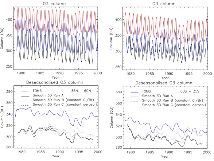
Fig. 3. Zonal mean column O3averaged between (top left) 35◦N–60◦N and (top right) 35◦S–60◦S from the 2D model (red line) and 3D

model run A (partial column, black line) compared with SBUV/TOMS monthly mean total column data (blue line) averaged over the same region. Panels (bottom left) and (bottom right) show the deseasonalised time series of TOMS/SBUV observations and the 3D model runs A, B and C. The deseasonalised values were obtained by subtracting the mean for each month (averaged over the whole run) and adding the annual mean (averaged over the whole run). All the datasets in panels c and d have been smoothed over 1 year.

amounts to 80 DU by 1998 relative to 1979. However, in the SH the model also fails to capture the observed interannual variability in the period 1994–1996. As noted above the ERA analyses finished in 1994 and this is a period when the oper-ational ECMWF analyses used to force the model were pe-riodically updated which can explain differences from 1994 onwards. Given that the results of Chipperfield and Jones (1999) showed good agreement of the NH March variability in the early 1990s, the discrepancies in March 1993 are likely also due to the impact of the analyses even though this is in the ERA15 period. This indicates that many years of simu-lation need to be compared to estimate the overall quality of CTM simulations.

Overall, based on the Fig. 2 and previous studies, the model appears to produce a realistic simulation of polar ozone in both hemispheres. This is a region where 3D models are expected to be better than 2D models. Given the likely

importance of the polar regions on mid-latitude ozone, this aspect is an improvement on such previous studies.

3.3 Mid-latitude column ozone

Figure 3 shows a comparison of zonal mean column O3in the

NH and SH mid latitudes from satellite observations and the model runs. The observations are the merged TOMS/SBUV dataset of R. Stolarski (personal communication, 2001). This dataset uses Nimbus 7 TOMS and SBUV, the NOAA 9, 11, and 14 SBUV/2 and the Earth Probe TOMS. Both the 2D model and the 3D model reproduce the timing of the an-nual cycle in the mid-latitudes, although the 2D model over-estimates the observations by about 40 DU. The 3D model partial column (above 350 K) is less than the observed to-tal column by about 30 DU which could be largely explained by including a tropospheric contribution. (The further col-umn differences with the 2D model just after the initialisation

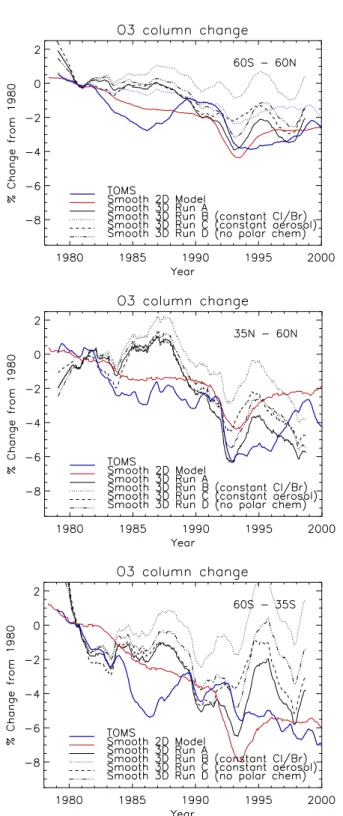
Fig. 4. Change in satellite-observed zonal mean, monthly mean col-umn ozone compared to 1980 averaged within latitude bands (top) 60◦S–60◦N, (middle) 35◦N–60◦N, and (bottom) 35◦S–60◦S. Also shown are model results from 2D run TD and 3D runs A, B, C and D. The 2D model output was saved every 25 days and the 3D model output was saved every 20 days. All the model results were smoothed over 2 years. The smoothing can cause the model change to appear non-zero in 1980.

date are due to the use of θ levels to convert the 2D model values to initial 3D model values; the 2D model does not have the same temperature field as the CTM). As expected the 2D model shows very little interannual variability, except during 1992–1993 after the eruption of Mt. Pinatubo when the peak O3column in both hemispheres decreased by about

20-30 DU. In contrast the 3D model shows much more in-terannual variability which is driven by the meteorological analyses used to force the model. This is shown more clearly in deseasonalised column O3comparisons in Figs. 3c and d.

The basic 3D model captures a number of variations which are seen in the observations. In particular, it is interesting to note that the 3D model does indicate a relative dip in SH mid-latitude O3during 1985. The modelled dip (of around

10 DU) is somewhat smaller than the observations, though it does indicate that this so-far unexplained feature in the ob-servations has at least partly dynamical origin.

Figures 3c and d also include results from the 3D model sensitivity runs. Over the 20 year model run, the chemical ef-fect of the increase in halogens leads to a reduction of around 20 DU in the SH and 10 DU in the NH. Note that as the model O3is used in the heating rate calculation which drives

the vertical transport, differences in O3between runs A and

B could potentially affect the circulation, causing further

dif-ferences between the two runs. However, using a coupled general circulation model with interactive O3, Braesicke and

Pyle (2003) found only a small feedback of long-term lower stratospheric O3changes on circulation. Therefore, we can

assume that the differences between runs A and B are domi-nated by the different imposed halogen trends.

Comparison of C, with constant (background) aerosol, with A indicates the chemical effect of aerosol variations on stratospheric ozone. Previously, using a CTM with pa-rameterised O3, Hadjinicolaou et al. (1997) argued that at

least some of the decrease in NH mid-latitudes after the Mt. Pinatubo eruption was “dynamical” in origin, though the analysed winds used to force the model may have contained perturbations due to the increased aerosol. In contrast, 2D models reproduce the post-Pinatubo NH decrease through increased chemical processing (e.g. see Chipperfield and Randel, 2003). Figure 3c shows that run C also produces a dip around 1993, confirming that information in the analyses makes a “dynamical” contribution to the observed decrease. However, the decrease is not as marked as in run A indicating a role for both direct aerosol-related chemistry and transport. This is discussed in more detail in Chipperfield (1999). Our run with constant (background) aerosol shows that the en-hanced aerosol increases the sensitivity of the atmosphere to the halogen trend. In the early 1990s the enhanced aerosol increased O3loss while in the early 1990s run C had more

O3than run A.

Figure 4 compares the observed anomaly (expressed as % change since 1980) for global (60◦N–60◦S), NH (35◦N– 60◦N) and SH (35◦S–60◦S) column ozone. (Note that the longer smoothing period used in Fig. 4 compared to Figs. 3c

removes the signal of the 1985 dip in the SH). Overall, model run A reproduces the observed decrease in column ozone in these three regions between 1980 and the early 1990s. In ad-dition some of the observed variability on the timescale of a few years is reproduced by the model, especially before the early 1990s. Later in the 1990s the modelled variations do not agree as well and this again is likely related at least in part to the changing ECMWF analyses. A notable feature of the 3D comparison in Fig. 4 are the differences with the observations in the mid 1980s; this is discussed in Sect. 3.4 (below).

3.4 Possible solar cycle effects

Global ozone observations display considerable interannual variability which is approximately in phase with the 11-year solar cycle. This variability is driven by changes in solar ul-traviolet irradiance which modifies the rate of odd-oxygen production in the mid-upper stratosphere (e.g. Huang and Brasseur, 1993). Observations show that the variation in col-umn ozone in the tropics is approximately 2–3% between solar maximum and solar minimum with relatively flat latitu-dinal structure (W. Randel, personal communication, 2002). Model studies (e.g. Huang and Brasseur, 1993; Flemming et al., 1995) also support this broad latitudinal structure to the solar cycle signal and produce a typical amplitude of 1.5–2% (solar maximum – solar minimum).

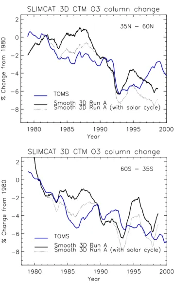
The 3D CTM used here does not contain a parameterisa-tion of the effects of the solar cycle; the solar fluxes used in the model’s photolysis scheme are fixed and taken from WMO (1985). Therefore, it is likely that some of the large deviations seen in the column ozone comparisons in Fig. 4 are due to solar cycle effects (which have not been removed from the observations). To test this, in Fig. 5 a solar cycle variation of 2% (solar maximum – solar minimum, in phase with the F10.7 flux) has been imposed on the results of A, assuming the WMO (1985) fluxes represent solar maximum conditions. The inclusion of the solar cycle effects signif-icantly improves the comparison with the satellite observa-tions during the mid 1980s and also during the mid 1990s – the periods corresponding to minima in the 11-year solar cycle.

3.5 Ozone profile variability

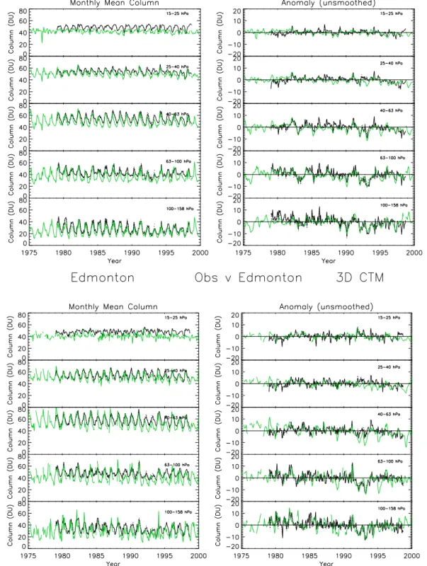
We now discuss how well the model captures the observed changes in ozone at different altitudes by comparing with long-term sonde records. Figure 6 compares the ozone from model run A with a time series of O3 sonde observations

at six different pressure levels at Hohenpeissenberg (48◦N, 11◦E) and Edmonton (53◦N, 246◦E) (Logan, 1999; Logan et al., 1999; personal communication, 2003). The observa-tions show a difference in the trend with altitude. At the higher levels at both sites there is a relatively continuous de-cline throughout the records. In contrast, in the lower

strato-Fig. 5. As strato-Fig. 4 for (top) 35◦N–60◦N, and (bottom) 35◦S–60◦S but for results of model run A with and without an assumed 2% (so-lar maximum – so(so-lar minimum) variation of column ozone during the 11-year solar cycle.

sphere, ozone shows a decrease in the early 1990s with rela-tively constant values thereafter.

The model reproduces the observed changes at the two stations well. The magnitude of ozone, and the phase of the annual cycle, is well captured, except at the highest level (15–25 hPa) where the model overestimates the obser-vations. This is near the top boundary of the 3D model. The model also reproduces much of of the observed variability and longer term changes. At 63–40 hPa the model repro-duces the essentially continuous decline, while at the lower altitudes the model reproduces the large negative anomaly in the early 1990s followed by a recovery. The model also re-produces the ozone minimum observed around 1983 (e.g. at 63–100 hPa at Hohenpeissenberg). At the levels above 40– 63 hPa both the observations and model show less variability (as the chemical lifetime of ozone becomes shorter) and less

Fig. 6. Left: Observations of monthly mean ozone sonde observations (green line) averaged onto ∼3 km layers for (top) Hohenpeissenberg (48◦N, 11◦E) and (bottom) Edmonton (53◦N, 246◦E). Also shown are the monthly mean results from model run A averaged over the vertical levels (black line). Right: Deseasonalised ozone anomalies on the same 6 pressure levels along with the results from model run A. Observed anomaly has 3-month running mean. In the top panel, the Hohenpeissenberg observations are compared with model output from the nearby Jungfraujoch station as this was one of the sites for which output was saved more frequently than the global fields. (Ozone data courtesy of J. A. Logan).

of an anomaly in the early 1990s. Especially in the lower stratosphere (LS), the success of the CTM in reproducing the O3variability is due to the quality of the ECMWF winds used

to forced the model. The results from this relatively coarse resolution model run are therefore encouraging. A higher horizontal resolution would, however, be expected to have an impact, and likely improve, the comparison.

Logan et al. (1999) discuss differences in the observations between European and Canadian sonde stations which are captured by the model. For example the model reproduces the minima in 1990, 1992, and 1993 over Europe, while over Canada only the last two of these are observed and modelled; in 1990 no minimum is occurs over Edmonton. The mini-mum in 1995 is not modelled at either location.

3.6 Mid-latitude profile changes

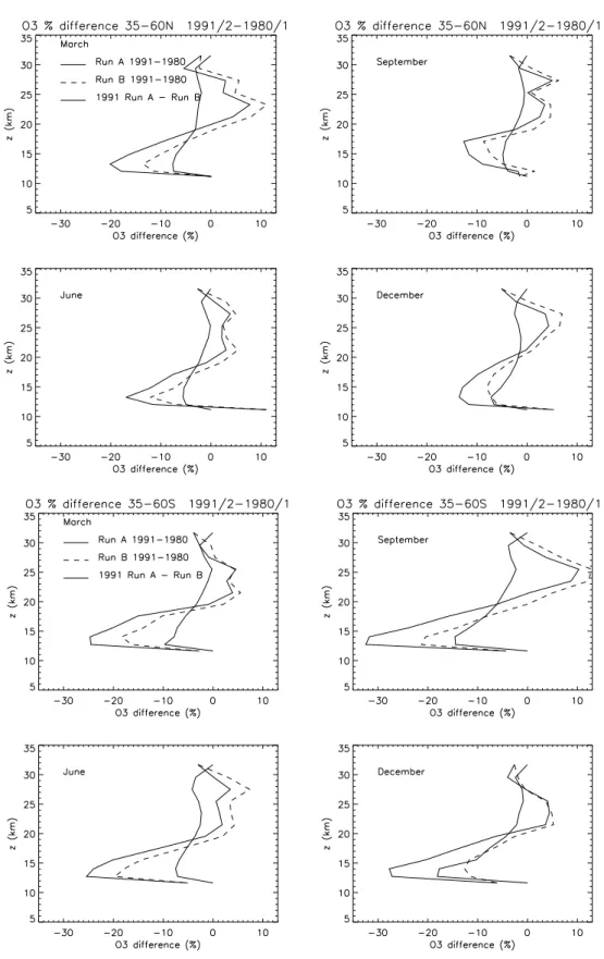
Figure 7 shows the percentage difference in zonal mean, monthly mean O3for the NH and SH mid-latitudes between

1991/92 and 1980/81 for runs A and B. (This restricts the differences to the ERA15 period and the monthly mean was averaged over two years to reduce any QBO effects). These differences include both the effects of chemical loss due to increased halogens over this time period (in run A) and me-teorological variability. Also shown in Fig. 7 is the profile difference between runs A and B for 1991. In this case the O3difference is just due to the difference in halogen loading

between these two runs and can be described as the (halogen-induced) “chemical loss”. These profiles show the largest signal of model O3chemical loss occurs in the lower

strato-sphere with another smaller depletion near the top boundary at 30 km. This profile shape is similar to profiles of the esti-mated trend (e.g. WMO, 1999) but is displaced to somewhat lower altitudes. In the NH this maximum LS chemical loss is around −8% in December–June and slightly less in Septem-ber. In the SH the differences are larger with a maximum of −19% in December. For the NH in March, Fig. 7a shows that the 1991/92–1980/81 LS differences for run A are much larger (−20%) than the chemical loss. This emphasises the effect of dynamical variability on changing the O3profile at

these lower altitudes. At other times of year the 1991/92– 1980/81 O3 profile differences in run A are more similar

to the chemical loss – i.e. the impact of dynamical vari-ability is slightly less. In the SH the 1991/92–1980/81 run

A differences are also different to the chemical loss. In this

hemisphere the impact of meteorological variability chang-ing the O3profile is least evident in December. Evidently

the difference in the O3profiles between two time periods is

strongly affected by meteorological variability (as in the col-umn comparisons in Fig. 4). The difference between the two model runs gives the cleanest signal of the modelled chemi-cal “trend”.

3.7 Ozone trends

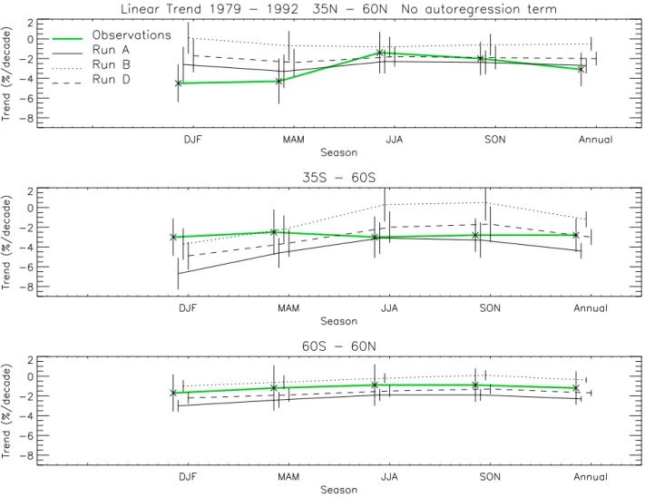
The trend model of V. Fioletov (described in WMO, 1998) was used to calculate linear trends of the model output from 1979 to 1992 over the latitude bands 35◦N-60◦N, 35◦S– 60◦S, and 60◦N–60◦S. This time period was chosen as it is a period over which the ECMWF analyses used to force the CTM were produced with a single meteorological model. The calculated trends for four seasons and the whole year are shown in Fig. 8 along with values for the merged satel-lite O3dataset. When applying the statistical model to the

CTM output the autocorrelation coefficient for the residuals for the 35◦S–60◦S and 60◦N–60◦S belts was about 0.95, while for 35◦N–60◦N and the observations the autocorrela-tion coefficient was around 0.75–0.8. To prevent large model error bars in the global and SH values the trend model was applied in two ways: with no autoregression term and with the autoregression coefficient specified with the observation value (0.77). Figure 8 shows the results which ignore the au-toregression term; results for the specified auau-toregression co-efficient (not shown) are very similar but with slightly more negative trends for the 35◦S–60◦S and 60◦N–60◦S regions. Overall, the magnitude of the trends from model run

A generally agree with the observed values (around 2–

4%/decade). Model run B which uses a constant halogen loading naturally shows smaller trends and the difference be-tween these two runs indicated the modelled halogen chemi-cal trend. Although the trends chemi-calculated from run B are of-ten still within the error bars of the observations, for 35◦N– 60◦N and 35◦S–60◦S the agreement is better between the observations and run A. Globally (60◦S–60◦N) the observed trends are smaller and both runs A and B lie within the error bars. For the NH in DJF however, although the model and observation error bars still overlap the model agreement is poorer. In the NH the observations indicate a maximum trend in the winter/spring period, while the model shows less sea-sonal variation. This underestimate in the springtime trend may be related to an underestimation of polar loss. This is a known problem of chemical models for winters in the mid-late 1990s (e.g. Becker et al., 1998) and may also occur in earlier winters.

In contrast, in the SH model run A exhibits more seasonal-ity in the trend (maximum negative trend in DJF) than the ob-servations which do not show much variation. The modelled trend agrees with the observations (within the error bars) ex-cept for this DJF period. The calculated trends from D in-dicate the effect of the large springtime polar loss (Fig. 2) on the mid-latitude trends. Although the difference between the trends from run A and run D is larger in SON (and DJF), run D also displays a similar seasonality to run A. Model run

B also display this seasonality with a trend near 0% in JJA

and SON and −4% in DJF. From this it would seem that the model’s chemical (halogen) signal of the SH trend is of a similar magnitude to the observed trend all year round, but other factors are causing a larger summer/autumn trend (see

Fig. 7. Percentage difference in the zonal-mean monthly mean ozone profile for March, June, September and December averaged over the latitude bands (top) 35◦N–60◦N and (bottom) 35◦S–60◦S. The panels show the percentage difference between the 1991/92 and 1980/81 profiles for run A (solid line) and run B (dashed line), and the percentage difference between A and B for the 1991/92 average (thick solid line).

Fig. 8. Estimated linear trends (%/decade) over the time period 1979-1992 from model runs A, B and D for 4 seasons and the whole year for (top) 35◦N–60◦N, (middle) 35◦S–60◦S and (bottom) 60◦S–60◦N. The error bars indicate the 2 sigma uncertainty. The statistical trend model used to analyse the CTM results did not include an autoregression term.

Fig. 7). This could be due to errors in the model dynam-ics during the summer/autumn causing the wrong transport of O3 or errors in summertime chemistry coupled with the

neglect of other chemical forcings.

4 Discussion

As discussed above, Hadjinicolaou et al. (2002) used a ver-sion of the SLIMCAT CTM with parameterised ozone chem-istry to investigate the role of dynamics on the long-term variability and trend of O3. They concluded that trends in

dy-namics have contributed strongly to the observed trend in NH mid-latitude spring time ozone. These conclusions appear somewhat contradictory to ours, although both studies have used similar models and data and so the model runs should be consistent. This apparent discrepancy is one of interpretation and can likely be explained by remembering that (i)

Hadjini-colaou et al. (2002) focused on NH spring, while our dis-cussion of the chemistry covers all seasons and hemispheres, and (ii) the agreement between the modelled and observed “dynamical tracer” time-series varies with the time period considered (possibly due to both real changes in the relative role of dynamics and changes in the ECMWF assimilation system). Hadjinicolaou et al. (2002) obtained the best fit to the column trends over the period 1998–1979. This is out-side of the ERA15 period and, due to dynamical variability anyway, there will be periods with better model/observation agreement than others. Here we concentrate on diagnosing the role of chemistry (through different model experiments) and wish to emphasise the problems and care needed in us-ing a CTM forced by analyses to quantify dynamical trends in ozone.

5 Conclusions

We have used a 3D off-line CTM to study the causes of the observed changes in ozone in the mid-high latitude lower stratosphere from 1979–1998. A series of model runs were performed to investigate the dependence of the modelled changes on trends in source gases, changes in aerosol and to diagnose the impact of polar processing on mid-latitudes.

Overall, the 3D model runs presented here support the con-clusion that trends in chlorine and bromine have been major causes of the observed decrease in mid-latitude ozone in both the SH and NH. These runs extend on previous 2D model simulations, however, in producing a better description of polar processes and capturing much of the observed (dynam-ically induced) variability.

The basic model performs well in reproducing the decadal evolution of the springtime depletion in the northern hemi-sphere (NH) and southern hemihemi-sphere (SH) high latitudes in the 1980s and early 1990s. After about 1994 the mod-elled interannual variability does not match the observations as well, which is probably due in part to changes in the op-erational ECMWF analyses. This indicates care needs to be taken when using such meteorological datasets to diagnose dynamical trends.

For mid-latitudes (35◦–60◦) the basic model reproduces the observed column ozone decreases from 1980 until the early 1990s. Model experiments show that the halogen trends dominate this modelled decrease and of this around 30– 50% is due to high-latitude processing on polar stratospheric clouds (PSCs). Dynamically induced ozone variations in the model correlate with observations over the timescale of a few years.

The model runs suggest that the 11-year solar cycle may play and important role in causing column ozone variations in mid-latitudes. Large discrepancies between the modelled and observed variations in the mid 1980s and mid 1990s can be largely resolved by assuming that the 11-year solar cycle (not explicitly included in the 3D model) causes a 2% (min-max) change in mid-latitude column ozone.

The runs presented here are a first attempt at applying a de-tailed 3D chemical model to the study of past mid-latitude O3

trends. In the future the availability of meteorological analy-ses over longer time periods and a larger vertical domain will permit more extensive studies.

Acknowledgements. We thank P. Hadjinicolaou, A. Jrrar and J.

A. Pyle for helpful discussions of their work and V. Fioletov for the trend calculations. We are also grateful to the coauthors of WMO/UNEP 2002 Chapter 4, in particular B. Randel, for useful discussions and J. Logan for supplying the sonde data. We thank R. Zander and E. Mahieu for the Jungfraujoch data. This work was supported by the UK Natural Environment Research Council and by the EU through the SAMMOA project (EVK2-CT-1999-000049). We thank the reviewers for their comments.

References

Becker, G., M¨uller, R., McKenna, D. S., Rex, M., and Carslaw, K. S.: Ozone loss rates in the Arctic stratosphere in the win-ter 1991/1992: Model calculations compared with Match results, Geophys. Res. Lett., 25, 4325–4329, 1998.

Braesicke, P., and J.A. Pyle, Changing ozone and changing circu-lation in northern mid-latitudes: Possible feedbacks? Geophys. Res. Lett., 30 (2), 1059, 2003.

Callis, L. B., Natarajan, M., Lambeth, J. D., and Boughner, R. E.: On the origin of midlatitude ozone changes: Data analysis and simulations for 1979–1993, J. Geophys. Res., 102, 1215–1228, 1997.

Chipperfield, M. P.: Multiannual simulations with a three-dimensional chemical transport model, J. Geophys. Res., 104, 1781–1805, 1999.

Chipperfield, M. P., Santee, M. L., Froidevaux, L., Manney, G. L., Read, W. G., Waters, J. W., Roche, A. E., and Russell, J. M.: Analysis of UARS data in the southern polar vortex in September 1992 using a chemical transport model, J. Geophys. Res., 101, 18 861–18 881, 1996.

Chipperfield, M. P. and Jones, R. L.: Relative influences of atmo-spheric chemistry and transport on Arctic O3trends, Nature, 400,

551–554, 1999.

Chipperfield, M. P. and Randel, W. J. (Lead Authors), Bodeker, G. E., Dameris, M., Fioletov, V. E., Friedl, R. R., Harris, N. R. P., Logan, J. A., McPeters, R. D., Muthama, N. J., Peter, T., Shep-herd, T. G., Shine, K. P., Solomon, S., Thomason, L. W., and Za-wodny, J. M.: Global Ozone: Past and Future, Chapter 4 in Sci-entific Understanding of Ozone Depletion: 2002, Global Ozone Research and Monitoring Project – Report No. 47, World Mete-orological Organization, Geneva, 2003.

Egorova, T. A., Rozanov, E. V., Schlesinger, M. E., Andronova, N. G., Malyshev, S. L., Karol, I. L., and Zubov, V. A.: As-sessment of the effect of the Montreal Protocol on atmospheric ozone, Geophys. Res. Lett., 28, 2389–2392, 2001.

Fleming E. L., Chandra, S., Jackman, C. H., Considine, D. B., and Douglass, A. R.: The middle atmospheric response to short and long-term solar UV variations – analysis of observations and 2d model results, J. Atmos. Terr. Phys., 57, 333–365, 1995. Hadjinicolaou, P., Jrrar, A., Pyle, J. A., and Bishop, L.: The

dynam-ically driven long-term trend in stratospheric ozone over northern mid-latitudes, Q. J. Roy. Met. Soc., 128, 1393–1412, 2002. Huang, T. Y. W. and Brasseur, G. P.: Effect of long-term solar

vari-ability in a 2-dimensional interactive model of the middle atmo-sphere, J. Geophys. Res., 98, 20 413–20 427, 1993.

Jackman, C. H., Considine, D. B., Chandra, S., Considine, D. B., and Rosenfield, J. E.: Past, present and future modeled ozone trends with comparisons to observed trends, J. Geophys. Res., 101, 28 753–28 767, 1996.

Kinnersley, J. S.: The climatology of the stratospheric THIN AIR model, Q. J. R. Meteorol. Soc., 122, 219–252, 1996.

Logan, J. A.: An analysis of ozonesonde data for the lower strato-sphere: Recommendations for testing models, J. Geophys. Res., 104, 16 151–16 170, 1999.

Logan, J. A., Megretskaia, I. A., Miller, A. J., et al.: Trends in the vertical distribution of ozone: A comparison of two analyses of ozonesonde data, J. Geophys. Res., 104, 26 373–26 399, 1999. Mahieu, E., Zander, R., Delbouillle, L., Demoulin, P., Roland, G.,

abun-dances of atmospheric gases from IR solar spectra recorded at the Jungfraujoch, J. Atmos. Chem., 28, 227–243, 1997. Newman, P. A., Gleason, J. F., McPeters, R. D., and Stolarksi, R.

S.: Anomalously low ozone over the Arctic, Geophys. Res. Lett., 24, 2689–2692, 1997.

Portmann. R. W., Brown, S. S., Gierczak, T., Talukdar, R. K., Burkholder, J. B., and Ravishankara, A. R.: Role of nitrogen oxides in the stratosphere: A reevaluation based on laboratory data, Geophys. Res. Lett., 26, 2387–2390, 1999.

Prather, M. J.: Numerical advection by conservation of second-order moments, J. Geophys. Res., 91, 6671–6681, 1986. Rinsland, C. P., Mahieu, E., Zander, R., et al.: Long-term trends

of inorganic chlorine from ground-based infrared solar spectra: Past increases and evidence for stabilization, J. Geophys. Res., (accepted), 2003.

Rummukainen, M., Isaksen, I. S. A., Rognerud, B., and Stordal, F.: A global model tool for three-dimensional multiyear strato-spheric chemistry simulations: Model description and first re-sults, J. Geophys. Res., 104, 26 437–26 456, 1999.

Sander, S. P., Friedl, R. R., DeMore, W. B., et al.: Chemical ki-netics and photochemical data for use in stratospheric modeling, Update to Evaluation no. 12, JPL Publ., 00-3, 2000.

Shine, K. P.: The middle atmosphere in the absence of dynamical heat fluxes, Q. J. R. Meteorol. Soc., 113, 603–633, 1987.

Solomon, S., Portmann, R. W., Garcia, R. R., Thomason, L. W., Poole, L. R., and McCormick, M. P.: The role aerosol varia-tions in anthropogenic ozone depletion at northern mid-latitudes, J. Geophys. Res., 101, 6713–6727, 1996.

Solomon, S., Portmann, R. W., Garcia, R. R., Randel, W., Wu, F., Nagatani, R., Gleason, J., Thomason, L., Poole, L. R., and Mc-Cormick, M. P.: Ozone depletion at mid-latitudes: Coupling of volcanic aerosols and temperature variability to anthropogenic chlorine, Geophys. Res. Lett., 25, 1871–1874, 1998.

Waugh, D. W., Considine, D. B., and Fleming, E. L.: Is upper strato-spheric chlorine decreasing as expected? Geophys. Res. Lett., 28, 1187–1190, 2001.

World Meteorological Organization (WMO): Scientific Assessment of Ozone Depletion: 1985, Global Ozone Research and Monitor-ing Project – Report No. 16, Geneva, 1985.

World Meteorological Organization (WMO): SPARC/IOC/GAW Assessment of Trends in the Vertical Distribution of Ozone, Har-ris, N., Hudson, R., and Phillips, C. (Eds), SPARC Report No. 1, WMO Ozone Rep. 43, Geneva, 1998.

World Meteorological Organization (WMO): Scientific Assessment of Ozone Depletion: 1998, Global Ozone Research and Monitor-ing Project – Report No. 44, Geneva, 1999.