Improvement of coarse root detection using time and frequency induced polarization: from laboratory to field experiments

HAL Id: hal-01730246

https://hal.archives-ouvertes.fr/hal-01730246

Submitted on 13 Mar 2018

HAL is a multi-disciplinary open access

archive for the deposit and dissemination of sci-entific research documents, whether they are pub-lished or not. The documents may come from teaching and research institutions in France or abroad, or from public or private research centers.

L’archive ouverte pluridisciplinaire HAL, est destinée au dépôt et à la diffusion de documents scientifiques de niveau recherche, publiés ou non, émanant des établissements d’enseignement et de recherche français ou étrangers, des laboratoires publics ou privés.

B. Mary, F. Abdulsamad, G Saracco, L. Peyras, M. Vennetier, P. Mériaux,

Christian Camerlynck

To cite this version:

B. Mary, F. Abdulsamad, G Saracco, L. Peyras, M. Vennetier, et al.. Improvement of coarse root detection using time and frequency induced polarization: from laboratory to field experiments. Plant and Soil, Springer Verlag, 2017, 417 (1-2), pp.243-259. �10.1007/s11104-017-3255-4�. �hal-01730246�

1

Improvement of coarse root detection using time and frequency

induced polarization: from laboratory to field experiments

Benjamin Mary1,2, Feras Abdulsamad3, Ginette Saracco2,4, Laurent Peyras1, Michel Vennetier*1,4, Patrice Mériaux1, Christian Camerlynck3

1

Irstea, unité de recherche RECOVER, 3275 route de Cézanne, Aix-en-Provence 2

CNRS – UMR7330, CEREGE, AMU, Equipe Modélisation, Europole de l’Arbois, BP80 F-13545 Aix-en-Provence-cedex4

3

Sorbonne Universités, UPMC Univ Paris 06, UMR 7619 METIS, Paris 05, France 4

ECCOREV FR 3098, Université Aix-Marseille, France * Corresponding author

Email address:

benjamin.mary@irstea.fr, feras.abdulsamad@upmc.fr, saracco@cerege.fr, laurent.peyras@irstea.fr michel.vennetier@irstea.fr *, patrice.meriaux@irstea.fr, christian.camerlynck@upmc.fr

Research highlights

1. We added induced polarization to the concept of classical resistivity to map in-situ root systems in soil.

2. Both TDIP and SIP are applicable for identifying root polarization.

3. High resolution images showed a correlation between root location and complex resistivity anomalies under semi-controlled conditions.

4. Using a frequency band provided useful information for locating coarse roots.

Abstract

Aims

Over the last decade the induced polarization (IP) method has emerged as a promising tool for subsurface investigation with growing interest for biogeophysics.

Methods

In this work, in addition to electrical resistivity methods, IP was tested experimentally as a proxy for identifying and discriminating tree coarse roots from the surrounding soil. This study permitted to show the effect of polarization at low frequencies (<25 Hz) using spectral (SIP) and temporal (TDIP) approaches both in laboratory and in the field.

Results

(i) the resistivity of woody roots samples was higher than that of a silty soil; (ii) the root polarized at frequencies lower than that of the soil; (iii) the effects of polarization increased with the volume of the buried roots (iv) the direction of roots relatively to current lines influenced the amplitude of IP response.

Applying the SIP method in-situ in semi-controlled conditions gave promising results since phase variations around 1 Hz frequency were correlated with buried root position.

Conclusions

SIP and TDIP approaches in the lab demonstrated their potential efficiency for detecting coarse roots. This was further demonstrated in field with SIP. Using maps at several frequencies was useful as variable environmental conditions may change the polarization relaxation frequency and amplitude. Additional works in semi-controlled conditions are necessary to study the dependence of IP response on different parameters of more complex and larger root systems.

Keywords

Coarse root detection; Electrical measurements; Induced polarization; Wood properties; Earth dike materials

2

Introduction

Understanding root development is of great importance for a wide range of disciplines including biology, agronomy (Allred et al., 2008; Amato et al., 2009; Green et al., 2006) and mechanical engineering (Dupuy et al., 2005; Ghestem et al., 2014; Stokes et al., 2009; Veylon et al., 2015). In civil engineering, understanding root development is essential for the safety of hydraulic structures such as river dikes and dams. Hydraulic structures built with earth fill (often silty) may be degraded by woody vegetation growing on them (Corcoran et al., 2010; Vennetier et al., 2015a, 2015b; Zanetti et al., 2009, 2011). The main coarse roots, especially those that cross the structure, are the most dangerous: they form a hole during their decomposition, inducing internal erosion that may lead to a breach (Foster et al., 2000). So far, ground penetrating radar (GPR) and electrical resistivity tomography (ERT) have been the methods used most frequently for imaging root systems and used to evaluate buried root mass (Guo et al., 2013) either for direct root detection or indirectly by monitoring soil drying due to root absorption. They have sometimes been tested to map root spatial distribution (Barton and Montagu, 2004; Loperte et al., 2006) but rarely root extension or architecture (Wu et al., 2014) though this would permit detecting isolated roots in embankment hydraulic structures. Root detection relies on:

(i) contrasts of dimension between the target and the surrounding material: many scales of heterogeneity are involved, especially in the case of embankment dikes and dams often composed of varied materials (Serre et al., 2008). A single coarse root may be embedded in different materials. Moreover, root systems are complex hierarchical systems composed of many interconnected roots of different sizes that adapt to soil conditions (Zanetti et al., 2015);

(ii) contrasts in the magnitude of physical parameters, linked to the intrinsic nature of soils and roots according to the type of source used. In the case of electric current (e.g., chargeability, resistivity), the external layers of bark and root heartwood (when present) are electrically insulating (Hagrey, 2007). As a result roots embedded in the soil appear mainly in the form of positive resistance anomalies (Amato et al., 2008; Zenone et al., 2008). The amplitude of contrasts varies according to the soil resistivity and tree species (Zanetti et al., 2011), to the water content and the decay state of the wood itself (Martin et al. 2012) and to variations in soil water content (Beff et al., 2013; Cassiani et al., 2015; Garré et al., 2011). Another proxy for detection is required and may be obtained using the properties of porous materials. Heterogeneous material can also be described by their dependence on frequency regarding the amplitude of conductivity and the phase shift between the injected signal and the resulting potential: this is the induced polarization method (IP), initially developed for mining prospection by Schlumberger brothers (Schlumberger, 1920), then for soil studies (Olhoeft, 1985; Vanhala et al., 1998). At frequencies lower than 103 Hz, the polarization mechanisms, that account for charge local displacement or reorientation when an extern electric field is applied, are either those linked to electrode polarization (redox reactions), or polarizations linked to the electric double layer (EDL) described by Chapman (1913); Gouy, (1910) and Stern (1924). Electrode polarization is linked to the coexistence of conduction made by electrons (from metallic particles) and ions contained in the electrolyte. Wood does not contain charge carriers like electrons since wood cells mainly consist of cellulose, which has a slightly negative surface charge. When the solid phase (surface charged negatively) is in contact with ions from the electrolyte an EDL layer is formed in order to reestablish the electro-neutrality. Depending of the size of the pores, the EDL may prevent movements of

3

large ions (selective zone) when an external electrical field induces the displacement of the anions and cations present in the electrolyte. In the selective zone, cations are stored and accumulate which causes a disequilibrium of the ionic concentration (Thierry et al., 2001; Weller et al., 2006). When stopping the electric field, the disequilibrium of the ionic concentration returns to normal by diffusion, thus producing the IP response measured. Several experiments have demonstrated that polarization of wood is governed by the macro and microstructure of wood cells and, related to its porosity (50-60% according to Niemz (1993)).

For wood samples alone as well as for tree stump measurements, Martin (2012); Schleifer et al. (2002) and Zanetti et al. (2011) showed a polarization peak lower than 25 Hz with variable amplitudes from 33 to 70 mrad depending on tree species and water saturation of wood (Table

2). Zanetti et al. (2011) showed that the amplitude of polarization depends on the species,

which porosity patterns differ greatly according to the size, shape and spatial distribution (homogeneous, concentrated in rings, at random, isolated or clustered) of sap conducting vessels (Schweingruber and Bosshard, 1982). Other parameters such as decomposition, water content and anisotropy govern the amplitude and frequency of the polarization peak. The decomposition of wood is characterized by the destruction of wood cells and a subsequent reduction of polarization effects (Martin and Günther, 2013).Following Martin et al. (2012) differences in the phase are mainly affected by the electrolytic conductivity (ions contained in the electrolyte). Thus amplitude and direction of polarization effects depend on the level to which the roots are saturated with water (free water and bound water). Amplitude of the phase when the sample is oriented in radial position is expected to be lower than measurements in axial position for which the current is transmitted along wood fibers and vessels since most of the fluid transports occurs in axial measurement directions.

When a current is applied into a medium with wood material embedded, polarization may have several origins: polarization due to the soil, an ionic gradient concentration at roots/soil interface and finally membrane polarization when current passes through the root as described above. Although the polarization phenomenon is also valid for clayey materials (Scott and Barker, 2003; Slater and Lesmes, 2002), it is expected that roots polarize more strongly than soil (Vanderborght et al., 2013), since the polarization of the soil is generally weak (<10 mrad) in metal-free soil (Zimmermann et al., 2008a, 2008b). According to Schleifer et al. (2002) the contrast in the module of resistivity is insufficient to detect an archeological woody plankway while the phase contrast is high. In conclusion, field IP measurements are expected to improve the success of in situ investigations of roots compared to ERT alone, especially when ERT presents limits such as in a resistive soil (low water content or resistive material).

Our objective in this study was to implement the IP method to detect and locate woody root in the soil. We focused on evaluating the experimental applicability of the method via experiments performed in the laboratory, and then in situ in controlled environments. The originality of our study lies in the combination of SIP (spectral induced polarization) and TDIP (time domain induced polarization) applied for the first time together in this context. The work was carried out on a set-up allowing a fast and relatively straightforward methodology to achieve two objectives: (i), to evaluate experimentally the IP response as a function of buried root mass using SIP and TDIP; (ii) to identify the preferential instrumental measurement domain (time or frequency) to be used for in-situ prospections to detect the presence of coarse roots, by evaluating the most discriminating physical parameters for each method.

4

Materials and methods

Measurement of polarization and comparison of spectral and temporal

approaches

Measuring in the time domain (TDIP)

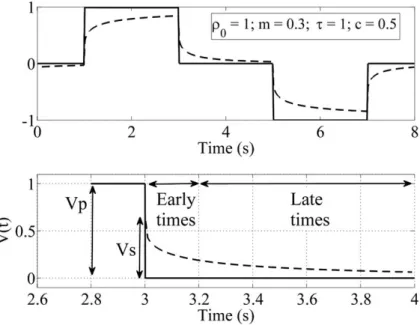
Acquisition of time domain IP data is technically similar to ERT (it provides data on resistivity and chargeability at the same time), but it is much more difficult from the standpoint of measurement due to the much smaller signal (Dahlin et al., 2013). The principle of time domain IP involves injecting a direct current (Figure 1) into the subsurface by using two injection electrodes. This current creates a potential difference in the soil which is measured by another pair of electrodes. The partial chargeability mi (in mV/V) is calculated

by integrating the decrease of the voltage V (Figure 1) with time by defining the windows between the times 𝒕𝒊

(1) 𝒎_𝒊= _𝑽 𝟏

𝒑(𝒕𝒊+𝟏−𝒕𝒊) ∫ 𝑽(𝒕) 𝒅𝒕

𝒕𝒊+𝟏

𝒕𝒊

with Vp the primary voltage measured just

before the current cut off (i.e. the potential used for DC resistivity), Vs the secondary potential.

The apparent total chargeability is defined by the sum of the partial chargeabilities .

(2) 𝒎 = ∑𝒏_𝒊=𝟏𝒎_𝒊 with n the number of partial chargeabilities

measured (n = 20 in Syscal-Pro used in this study).

The measured chargeability depends on the properties of the medium and the time of current (Ton) transmitted (Gurin et al., 2013; Johnson, 1984). The choice of Ton must take the constant

of time τ characteristic of the anomaly into account (or its inverse the relaxation frequency, cf.

Figure 2b and the Cole-Cole model below). The longer τ is, the larger Ton must be in order to

measure the polarization correctly.

Figure 1: Illustration of polarization effect during TDIP measurement (ρ0 in Ω.m, m in V/V, τ in s, c is dimensionless): rectangular current injection (plain line) and simulated voltage response (dashed line determined with arbitrary Cole-Cole parameters using the equation of Duckworth and Brown (1996). (b) Selection of one shut-off time window illustrating Vp and Vs (inspired by Gurin et al. (2013))

5

Measuring in the spectral domain (SIP)

In the frequency domain, an alternative sinusoidal current of known frequency f (or pulsation ω = 2πf) is injected between the injection electrodes and induces a voltage response which is also sinusoidal but delayed compared to the current (Figure 2a). The results are expressed in terms of resistivity modulus |ρ(ω)| (or conductivity) and phase φ (Figure 2b) according to equation 3 or equivalently equation 4:

(3) 𝝆(𝝎) = 𝝆′(𝝎) + 𝒊𝝆″(𝝎) (4) 𝝆(𝝎) = |𝝆(𝝎)| 𝒆−𝒊𝝋(𝝎)

where ρ' and ρ″ are the real and the imaginary parts (i=√−𝟏√−𝟏) of the complex resistivity respectively, |ρ| is the modulus (Ω.m) and – φ is the phase (rad).

Figure 2: (a) Illustration of polarization effect during the SIP measurement: one injected sinusoid current and the voltage response shifted in phase (φ);

(b) Phase of the complex resistivity (derived from equations 2 and 3). Influence of chargeability (m) and time constant (τ) characteristics of the medium on relaxation frequency (fr)

Comparison of the two domains

Types of IP measurements differentiate because: (i) SIP allows measurements of polarization processes occurring between 0.001 Hz and 20 kHz whereas TDIP, with classical instruments, is limited to a frequency range between 0.25 Hz and 64 kHz according to Florsch et al. (2011); (ii) generally, TDIP carries out the measurement with a single time of injection, whereas with SIP, the section of complex resistivity is obtained with the whole range of desired frequencies; (iii) in real conditions, sites can be subject to considerable compaction (especially at the crest of a dike) and it is much more practical to use stainless steel electrodes.

6

Unfortunately these electrodes polarize, adding noise to soil signal. However, Dahlin et al. (2013) and Hördt et al. (2007) showed that the use of non-polarizable electrodes in-situ with TDIP does not give better results when: (1) the study site has low electrical resistivity; (2) the electrodes used for injection are not used immediately for the following potential measurement. The TDIP approach appears easier to implement on a dike.

Cole-Cole model

A number of phenomenological models exist that can be used to fit the IP spectra, among which the most commonly used is the Cole–Cole model (CCM) (Cole and Cole, 1941; Pelton et al., 1978). The Cole–Cole model assumes that the polarization spectra exhibits a peak frequency (𝑓_𝑟) (Figure 2) and involves four parameters describing the shape of this spectrum.

The Cole–Cole model describing the complex resistivity ρ*(ω) 𝝆∗(𝝎) in the frequency domain is given by equation 5: (5) 𝝆∗_{(𝝎) = 𝝆} 𝟎[𝟏 − 𝒎 (𝟏 − 𝟏 𝟏 + (𝒊𝝎𝝉)𝒄)]

with ρ0 (Ω.m) the direct current resistivity modulus, m the chargeability, τ (s) the time constant, c (dimensionless) is a so-called CCM exponent, ω (rad) is the angular frequency and i the imaginary unit.

Pelton et al. (1978) showed that in the time domain intrinsic chargeability curves m (t) can be describes by equation 6:

(6) _Where

_m

chargeability taken at t = 0 ( m(t = 0)) and Γ is the Gamma function.

The inversion of Cole-Cole parameters in the time and frequency domains was thoroughly investigated, using both the least squares method and the Bayesian approach (Ghorbani et al., 2007; Hönig and Tezkan, 2007; Kemna et al., 2000; Yuval and Oldenburg, 1997). For this study, voltage decay curves from TDIP measurements were first fitted using the Cole-Cole parametric function defined by Pelton et al. (1978) in time domain (equation 6). A fitting algorithm, based on the minimization of the cost function using a least squares criterion was then computed in Matlab®. The initial values of the four parameters of the model were constrained allowing it to converge to physical acceptable values. To achieve this, ρ0 was fixed by the value of the corrected resistivity modulus, whereas m is contained between 0 and 0.1. This range was defined for a nonmetallic medium according to Ghorbani et al. (2007), whereas τ could vary between 0.01 and 1000 s according to Loke et al. (2006). Consequently the knowledge of parameters permitted modeling the frequency response (from equation 5 above), and comparing the measurements of different domains.

Laboratory measurements

The first two steps of this study were performed in the laboratory: (i) first on root samples alone to determine their electrical properties and differences relative to soil, (ii) then on roots embedded in the soil with different proportions of buried roots.

For the laboratory experiment, 20 cm-long poplar root samples (P) of various diameters (8-25-30-35 and 50 mm = P-8 to P-50) were cut from stumps extracted on different French dikes. Their fresh weight was recorded and part of them were kept in plastic bags in the dark for a few weeks for this experiment. The other ones were dried to measure the initial water

7

content of the roots. At the time of measurement, root samples were weighed again and root water content was inferred from their initial weight and the water content of subsamples which were fully dried just after sampling, assuming that the variations of mass were caused only by the loss of water. The water content of root samples ranged from 17 to 30% of the dry wood.

Set-up for measurements on root alone

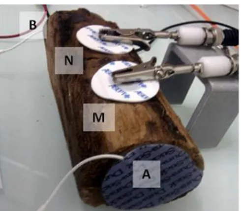
The measurements were performed on a root sample of poplar 35 mm in diameter (P-35). The experimental set-up was that proposed by Cosenza et al. (2007) and Ghorbani et al. (2009) and used for their measurements on argillite rock sample. This set-up consists of medical electrodes made of a carbon film placed in contact at the extremities of the sample to inject the current. This methodology allows conserving the whole sample, rather than working on a standardized core. The patches (Valutrode® electrodes from Axelgaard Manufacturing Co.), on which were placed a carbon mesh (50 mm diameter, 1mm thick) containing a coupling agent (AgCl gel), allowed: (i) preventing biases related to connection resistances; (ii) limiting the current to that transmitted by ions contained in the sample (which is not possible when coupling is ensured by water) and (iii) a homogeneous injection through the root. Two other electrocardiogram (ECG) type, non-polarizable Ag/AgCl electrodes (Asept Co.) were placed along the length of the root to measure the voltage drop (without removing the bark to be close to real conditions). The electrodes formed a Wenner α type system (i.e. a line of four equally spaced electrodes). So that the sample was analyzed in its axial direction: current was injected through the outer electrodes (AB) and potential was measured between the inner electrodes (MN), cf. figure 3.

Figure 3: Transmission measurement of sample P-35 using a Wenner α type set-up composed of medical electrodes; AB are injection electrodes (carbon, Ag/AgCl film), and MN the potential measurement electrodes.

Time and frequency domain measurement devices

The TDIP measurements were performed using a SYSCAL Pro® (Iris instrument) for an injection period of 4s. The voltage was set freely by the instrument in order to obtain a minimum current. The SIP measurements were performed using a SIP FUCHS III® (Radic research instrument) and a LIPPMANN® which is very easy to implement in-situ and was used for field experiment (IP Earth Resistivity Meters 4 point light 10W) in the frequency range between [0.001-103] Hz and [0.26-25] Hz respectively. Before measuring on the samples, the instrument was calibrated on an electric circuit of known response (Abdulsamad et al., 2016). Each sample was analyzed three times consecutively to evaluate the reproducibility of the measurement. On average, the measurement was stable with maximal variations of 0.1 mrad on the measured phase between each repetition. Thus plotted curves resulted from the average of the 3 measurements. The soil measurement used as reference was performed using the system presented below.

8

Set-up for measurement on root embedded in soil

Figure 4 illustrates the cylindrical sample holder (height 30 cm, diameter 20 cm) used to

measure the roots buried in soil initially designed by Okay (2011) for measurements on clays. This was done using a quadrupole electrode set-up placed in equatorial configuration. This geometry requires a geometric correction coefficient of K=0.45 determined with the COMSOL Multiphysics® software by Okay (2011). Non-polarizable electrodes formed by a copper-copper sulfate (Cu-CuS04) pair were used to measure the potential, whereas stainless

steel electrodes were used to inject the current.

Figure 4: Set-up for measuring polarization in the transversal direction of a root sample buried in soil. Description of the sample holder inspired by Okay (2011) showing the geometry of injection electrodes A and B (stainless steel), and the potential measurement electrodes M and N (non-polarizable CuS04); and the central position of the root sample.

The sample holder was filled to a height of 15 cm with a natural soil representive of dike earth fill, mostly silty with equivalent fractions (~20%) of sand and clay (Table 1). The water content of the soil, measured using a probe (WET-2- Sensor DeltaT Devices) was 10%. The soil was compacted by a press having a fixed mass for all samples.

Table 1 Soil grain size distribution. The granulometry is determined according to standards NF P 94–056 and NF P 94– 057 for sieving and sedimentation, respectively

The reference measurement was performed in the sample holder filled only with soil. Root samples of the same length (20 cm) and with increasing diameters were then introduced into the tank (Figure 4). The root sample was introduced in the transversal direction (transversal to the direct measurement of the sample). The samples varied between 8 and 50 mm in diameter (P-8 to P-50), i.e. 4 to 25% of the soil volume integrated by the measurement in the sample holder. These proportions of root volume provided a relatively realistic picture of superficial coarse roots, as studied in situ. Drill a hole (diameter slightly lower than root) disturbed the medium, which was systematically re-compacted by a press having a fixed mass. The evolution and the repeatability of the measurement during the experiment for the SIP and TDIP measurements were assessed with four different intermediate measurements (numbered

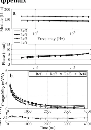
Ref1 to Ref4) on the soil alone at regular time intervals (Figure 9). The differences observed

between each of these measurements were used afterwards to determine the confidence intervals on the reference (50 Ω.m and 0.8 mrad at 1 Hz for the SIP measurement (SIP FUCHS III) and 0.5 mV/V (for TON=4 s) for the TDIP measurement (Syscal Pro) as shown in Figure 9 in appendix). For each root diameter and for an injection period of 4 s, the decay of the voltage was integrated with 20 time windows discretized logarithmically into time periods of [40-530] ms (i.e 3820 ms time recording in total) to obtain a better signal to noise ratio. A delay of 20 ms was applied before the first measurement of the voltage decay. Two series of SIP measurements were performed with the SIPFUCHS III to determine the conductivity modulus and phase in the range [9.10-2-103] Hz.

Granulometry/ Sedimentology <2 μm clay 22.7% 2 μm - 50 μm silt 51.6% 50 μm - 2 mm sand 19.2% 2 mm - 100 mm gravel 5.8%

9

Measurements under semi-controlled conditions

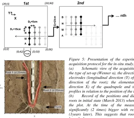
The study site was a grassland located in Aix-en-Provence, Southern France (N43°31'24.0"N, E5°30'42.0"E). Poplars (Populus Alba L. four year-old) were planted in large rectangular holes (Length x Width x Depth: 3x1x1m), filled with the same homogenous material as that used for the laboratory experiments (Table 1). Some holes were not planted in order to serve as controls. The tests were performed one year after planting. The first measured tree was 2.5 m high with a 15 cm diameter trunk at root collar. Its root system at plantation time was composed of two main superficial roots (Figure 5b) 20 and 25 mm in diameter at about 10 and 15 cm depth in the lengthwise direction of the plantation hole, and several other smaller roots oriented in the opposite direction. At the time of the measurement trees were significantly (2 times) bigger with respect to initial size (1 year later). This suggests that roots were bigger and branched.

Figure 5: Presentation of the experimental plot and the acquisition protocol for the in-situ study.

(a) Schematic view of the acquisition protocol showing the type of set-up (Wenner α), the direction of the quadrupole electrodes (longitudinal direction (Y) of the plot = assumed direction of the root); the elementary displacement (in direction X) of the quadrupole and the positions of two profiles in relation to the position of the trunk.

(b) Record of the positions and diameters of the main roots in initial state (March 2013) when planting the tree in the plot. At the time of the measurement trees were significantly (2 times) bigger with respect to initial size (1years later). This suggests that roots were bigger and branched

In-situ acquisition protocol

The first measurements were performed in January 2015. We made an horizontal mapping, with a median depth of penetration of 8 cm (Edwards, 1977) linked to a constant electrode spacing of 15 cm (Dy) using a Wenner α type set-up (Figure 5b). The arrangement of the

electrodes and the meshing of the measurements took the information on the initial position of the two large superficial roots into account, by assuming that their depth and direction had not changed. The electrodes (9 cm stainless steel nails) were fixed on a support to ensure constant distance and penetration in the soil. According to Dahlin et al. (2013) and Hördt et al. (2007), the system formed by the two injection electrodes and the two others used only for measuring the potential could lower electrode polarization effects. Four 1 m-long linear transects were

10

made across the width of the plot, i.e. perpendicular to the roots (Figure 5). Transects were spaced out 20 cm (Dl) and measurements were performed every 5 cm (Dx) along the transects

by translating the quadrupole electrodes. Measurements between profiles overlapped (in the y direction) hence one point to the neighbor point should be correlated. Points were interpolated using the kriging method which takes the spatial correlation into account.We choose to work with the LIPPMANN instrument, for which results obtained in laboratory were similar to SIP device and easier to set up in-situ. Each measurement point was repeated for each frequency (from 0.25 to 25 Hz) until the difference in amplitude between two successive measurements was lower than 0.1% (on the modulus) else at least 20 times. A similar map was made with an interval of one day according to the same protocol on a non-planted control plot under the same experimental conditions: neither precipitation nor difference in temperature was observed between the two days.

Results of laboratory and in-situ measurements

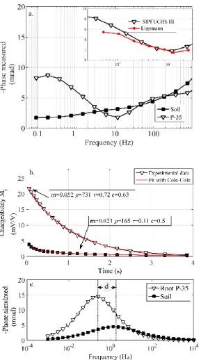
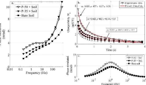
Figure 6 shows the results of the SIP measurements (6a), TDIP measurements (6b) and

simulated SIP measurements (6c). The comparison for each type of measurement was made between the P-35 sample and the measurement in the sample holder containing only soil.

Figure 6: Comparison of measurements on root sample P-35 with the reference measurement of the soil sample alone. Each sample was measured several times to ensure reproducibility.

(a) In the spectral domain, using SIPFUCHS (in black) and LIPPMANN (in red) – size of the uncertainties (0.1 mrad) are lower than marker size.

(b) In the time domain, for an injection period of 4 s; the solid red line shows the fit with the generalized Cole-Cole of voltage decay (with ρ0 in Ω.m, m in V/V, τ in s and c is dimensionless)

Figure 6a shows that the phase spectra for

measurement on the root alone and on bare soil were significantly different, their relative differences being much higher than the instrument errors, as well as the repeatability interval (0.8 mrad at 1 Hz). For the root alone, the maximum phase was located at about 0.2 Hz and the phase amplitude was about 9 mrad. For the soil-alone phase spectrum, no peak could be seen and the phase increased non linearly with the frequency, with no phase higher than 6 mrad over the frequency range lower than 400 Hz. At 0.1 Hz, the difference in amplitude between the soil sample and the root was 7 mrad. The most important result of these direct measurements was in the frequency range [0.1 - 10] Hz, for which the soil and root responses varied in opposite directions: when the frequency increased, the phase increased for the soil, whereas it decreased for the root sample. The

11

effects of the soil in comparison to the root sample predominated on the phase amplitude between 4 and 40 Hz, and for all frequencies above 200 Hz. However, the frequencies above 100 Hz could not be interpreted since the measurements were subject to undesirable effects caused by the set-up and probably due to heterogeneities at the interface electrode/samples (Abdulsamad et al., 2016). This explains the difference between the modeled response in figure 6c and the measured response in figure 6a. The measurements performed with the LIPPMANN (Figure 6) showed trends very similar to that obtained with the SIPFUCHS. However, lower polarization amplitudes (< 1 mrad) were observed with the LIPPMANN below 1 Hz.

Figure 6b illustrates the comparison between the decay curve of soil chargeability (msi) and that of the root sample (mri). This result is the equivalent, but in time domain, of results presented in Figure 6a. The differences were significant between the two decay rates when considering the uncertainty of measurements (about 0.5 mV/V) determined from Figure 9

Figure (in annex). The initial chargeability was higher on the root sample. According to

the fitted Cole-Cole parameters, the root differs from the soil by a higher resistivity modulus ρ (731 Ω.m on the root versus 165 Ω.m in the soil) and by a higher total chargeability (m), since mri was approximately 2.5 higher than msi (0.021 V/V versus 0.05 V/V). Differentiation was

also possible using the characteristic time constant, with τri higher (0.72 s) than τsi (0.11 s). According to table 2, the measured values (Figure 6a) were in accordance with those of the simulated spectrum (Figure 6c): the peak of the phase spectrum of the root was located at a lower frequency than that of the soil (f=0.2 Hz versus 0.9 Hz) and at a stronger amplitude (12 mrad versus 2 mrad). Thus results in time confirm those in frequency domain for which the same trends between soil and roots was observed but not the details of the variation.

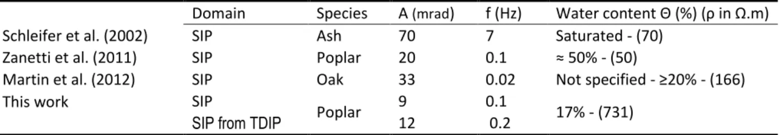
Domain Species A (mrad) f (Hz) Water content Θ (%) (ρ in Ω.m)

Schleifer et al. (2002) SIP Ash 70 7 Saturated - (70)

Zanetti et al. (2011) SIP Poplar 20 0.1 ≈ 50% - (50)

Martin et al. (2012) SIP Oak 33 0.02 Not specified - ≥20% - (166)

This work SIP

Poplar 9 0.1 17% - (731)

SIP from TDIP 12 0.2

Table 2: summary and comparison of the amplitude of the phase (A) in mrad (measured or calculated) and the relaxation frequency (f) in Hz with previous works on SIP measurements on root samples analyzed in the axial direction. Water content Θ (%) expressed on fresh weight basis. Meaning of ρ, φ and m are described in Figure 2

Measurement on root with soil: influence of root mass on resistivity and phase

Figure 7 shows the results of the SIP measurements (7a), TDIP measurements (7b) and

simulated SIP response derived from the Cole-Cole parameters (7c). For each of them a comparison was made between soil with root samples (P-35 and P-50) and soil without roots.

In Figure 7a, the phase spectra with root embedded in soil differs significantly from the soil alone, particularly between 0.2 Hz and 20Hz where the phase of the two root samples was higher than that of the soil in proportion to the diameter of the sample (ratios of 1.52 for P-50 and 1.48 for P-35 at 1.4 Hz, frequency for which ratio are the highest). Above 25 Hz, non-desirable induction effects made the interpretation impossible. On sample P-50 the local maximum of 4 mrad located at 3 Hz appears clearly whereas it did not stand out for sample diameters ≤35 mm. For sample diameters ≤30 mm (Table 3) the phase spectra was within the confidence range (Figure 9a) of the soil curve.

12

Figure 7: Comparison of measurements on root samples P-35 and P-50 buried in the sample holder (in the transversal direction) with the reference measurement of the soil only. Each sample was measured several times to ensure reproducibility.

(a) In the spectral domain; the sizes of the uncertainties (0.1 mrad) are lower than marker size.

(b) In the time domain, for an injection period of 4 s; the solid red line shows the fit with the generalized Cole-Cole of voltage decay (with ρ0 in Ω.m, m in V/V, τ in s and c is dimensionless).

(c) Simulation of the SIP response derived from the four Cole-Cole parameters fitted on fig (7b) in time domain.

In the time domain (TDIP), chargeability decay curves were significantly different between measures with and without roots (Figure 7b) only for P-50. This difference increased with root sample diameter, especially when considering the initial chargeability and early times on the curve. As shown in table 3, the fitted chargeability (m) and the time constant (τ) allowed respectively for the same and a better ratio coefficient discrimination of the samples than resistivity (ρ). The position of the simulated phase peak (Figure 7c) was located at a slightly lower frequency (1Hz versus 3 Hz), and at a higher amplitude than those obtained on the measured phase.

Table 3 shows that for the sample holder experiment the higher the volume of the root

introduced, the more charged the medium became in comparison to soil (mr/ms), ranging

between 1.02 and 1.47 (in TDIP and approximatively the same for the phase in SIP) for a 4 to 25% root/soil ratio. For both TDIP and SIP approaches, the ratio was not significantly different for root diameter lower than 30 mm (within the uncertainties range considering the evolution of the soil). No relationship between diameter and Cole-Cole parameters has been computed since the number of samples analyzed was insufficient. Nevertheless a slight trend may exist, phase and resistivity increasing with the diameter except for P-30. No trend was observed for relaxation time. No changes in these relationships were found when considering the total surface area of the sample instead of its mass or diameter.

13

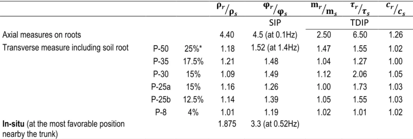
Table 1: ratio of physical quantities measured using spectral and temporal (Injection time=4s) approaches with three experimental steps: on the sample, in the sample holder (ranging from the biggest (P-50) to the smallest diameter (P-8) for respectively 4 to 25% volume occupied* or 0.026 to 0.20 cm2 of surface) and in-situ. Meaning of ρ, φ and m are described in Figure 2. 𝛒𝒓 𝛒𝒔 ⁄ 𝛗𝒓 𝛗𝒔 ⁄ 𝐦𝒓 𝐦𝒔 ⁄ 𝝉𝒓 𝝉𝒔 ⁄ 𝒄𝒓 𝒄𝒔 ⁄ SIP TDIP

Axial measures on roots 4.40 4.5 (at 0.1Hz) 2.50 6.50 1.26

Transverse measure including soil root P-50 25%* 1.18 1.52 (at 1.4Hz) 1.47 1.55 1.02 P-35 17.5% 1.21 1.48 1.04 1.27 1.00 P-30 15% 1.09 1.49 1.12 2.06 1.05 P-25a 15% 1.16 1.26 1.00 1.73 1.03 P-25b 12.5% 1.14 1.39 1.05 1.55 1.03 P-8 4% 1.01 1.19 1.02 1.01 1.02

In-situ (at the most favorable position

nearby the trunk) 1.875 3.3 (at 0.52Hz)

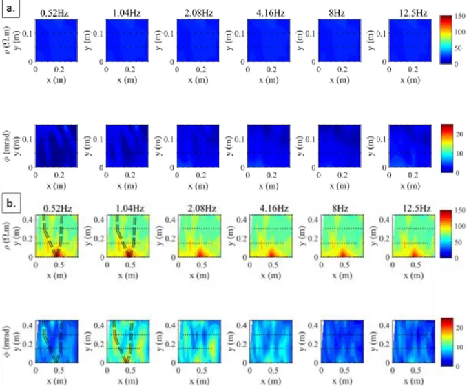
In-situ mapping of roots

The results are presented in the form of a two dimensional map (Figure 8) corresponding to the apparent resistivity and phase values for an horizontal 15 cm-deep layer, i.e. the estimated average depth of the roots. The color scales are the same for the control and the planted plot to facilitate their comparison. The resistivity modulus ρ was relatively low in the control plot, between 30 and 45 Ω.m (Figure 8a), clearly corresponding to the resistivity of a silty material. No spatial trend could be distinguished, and the soil appeared very homogeneous over the whole section whatever the space and frequency. Likewise, the variations observed for the phase (Φ) did not appear to indicate a preferential direction. However, it is noteworthy that at low frequencies (for 0.52 and 1.04 Hz), these variations of phase appeared to be correlated to resistivity. As the frequency increased, the entire plot became more highly charged to reach a maximum at ≃5 mrad.

For the planted plot (Figure 8b), there was a clear correlation between the resistivity modulus, the phase and the theoretical position of the two main roots (represented in doted lines). These two roots caused a resistivity anomaly of 130 Ω.m and positive phase anomaly of 18 mrad (at 1.04 Hz) nearby the trunk (x=0.5, y=0 cm). Farther, from 15 to 40 cm from the trunk, the distance increasing between the two main roots, the cumulative effect of superimposed roots disappeared and the resistivity varied from 70 to 100 Ω.m. The anomaly indicating the probable presence of root mass appeared more clearly at low frequencies, with the phase ranging from 10 to 18~mrad at 1.04 Hz, whereas it was only 6 mrad at 12.5 Hz (the same order of magnitude as the maximum amplitude observed on the reference plot). This was the expression of the effects of soil polarization observed on the reference plot. The position of the anomaly centered on the plot (X=0.5 m) and its extent (± 20 cm) clearly corresponded to the position and to the diameter of the two main roots. This anomaly extended in the longitudinal direction (Y). Farther than 20 cm from the trunk, the two roots could no longer be clearly differentiated from the soil, especially the smallest one and particularly for ρ. Moreover, an area of higher phase (15 mrad at 2.08 Hz at x=0.6 m; y=0.15 m) did not reflect the initial position of the main roots.

14

Figure 8: Result of the SIP map produced using the LIPPMANN device (a) on the reference plot with the soil alone (b) on a plot with the study tree. For each of them, the 1st line corresponds to the amplitude of resistivity (ρ), the second line to the amplitude of the phase (Φ). The injection frequency increases when looking from left to right of a line.

Discussion

Comparison of SIP and TDIP approaches in the laboratory

The resistivity modulus permitted discriminating soil samples (ρs=165 Ω.m, mostly silty,

with a water content of 10%) and woody root sample (ρr= 731 Ω.m, with a water content of

about 17%) with a ratio of 4.4. According to Palacky (1988) the resistivity of silts can reach 700 Ω.m when dry and if root water content increases (and its resistivity decreases), the soil/root discrimination in this case would be no longer possible using the resistivity modulus. As summarized in table 2, the direct measurements on the root samples did not result in a polarization peak similar to that obtained during previous studies on root of ash (or oak) analyzed in the same direction (axial). In particular, in comparison with the study by Schleifer et al. (2002), the amplitude was lower (10 mrad vs 70 mrad) and the polarization peak occurred at a lower frequency (0.2 Hz vs 10 Hz). The main difference is that the water content of wood samples was far higher in previous works. Logically, this points the preponderance of sample water content in the analysis of soil/root samples regarding both amplitude and the

15

position of the maximum phase of the spectral peak. When simulating the SIP response as a function of the Cole-Cole parameters estimated from the discharge curve, the amplitude and frequency of the polarization of the soil and root samples are comparable to those obtained by the SIP experimental measurement (Table 2). This result shows that both approaches are consistent and can be considered in-situ.

Parameter c varied slightly around 0.5. As can be seen in table 3, the most discriminant factor is the rate of decay (τ): on the root sample, τ is 0.6 s higher than for the soil (i.e. a ratio of 6.5). The chargeability (m) can also differ between the two types of samples (soil and root): the roots are more charged initially and globally (since τ is higher).

For the experiment on roots embedded in the soil, the IP response is expressed as a function of root diameter (equivalent to their volume or surface area in this case), representative of coarse roots. The response would not be the same for an equivalent volume of fine roots since the root surface area would be far higher. The maximum root/soil chargeability ratio of 1.47 and phase ratio 1.52 (at 1.4 Hz) were observed for a proportion of root of about 25% of the total volume. At 1.4 Hz, SIP polarization effects are approximately the same than with TDIP. In that experiment, with an increase of the surface area of the roots, both the ionic gradient concentration at roots/soil interface and the membrane polarization might act on amplitude of the polarization observed.

The comparison between the direct measurements on the sample and those performed on the sample holder showed that the results were consistent. Spectral characteristics of root P-35 showed a polarization peak of 9 mrad at 0.2 Hz (Figure 6). This root was buried in a medium which, at this frequency (0.2 Hz), was charged only at 2 mrad. In the sample holder experiment, which is the contribution of both root and soil polarization, the phase range 2-3 mrad (at 0.2 Hz) and mostly reflects the soil properties, as does the phase peak which shifted to higher frequency. For some samples, the effects of polarization for a buried root are of the same order of magnitude as those of the soil: the sample is analyzed in the transverse direction, corresponding to the anisotropy direction for which the polarization is lowest (e.g Introduction section) and including a large quantity of soil. This result is consistent with the study by Schleifer et al. (2002) who also obtained, confounded polarization effects. SIP and TDIP analyses give consistent results, so that both methods appear to be well adapted for highlighting the polarization effects of root systems in-situ. However, the information provided by SIP is better adapted for root/soil discrimination, since it covers a wider range of polarization.

Consistency of laboratory and in-situ results

During the in-situ measurements (carried out with SIP to show the frequency effects), the root is integrated in its longitudinal direction to maximize polarization effect, since the measurement quadrupole is oriented in a direction close to that of the root. Since the current is parallel to root fibers, this configuration is favorable for obtaining the maximum polarization effects reaching up to 18 mrad. This value is higher than that obtained in the laboratory, and can be explained by a higher root water and sap content in-situ and more root volume proportion in soil. Nevertheless at greater distance from the trunk (>20-30 cm), the electrical anomaly was less apparent particularly on the resistivity term. This can be explained by the decrease in diameter of the main roots with distance to trunk, which also branch out as they spread from the trunk. Their percentage in mass and volume in relation to the soil thus decreases with distance to trunk and the effects are increasingly dominated by the response of the soil.

16

In addition, the depth of the roots increases probably slightly with the distance to trunk and their ends corresponds to the limit of the set-up depth of investigation. With changes of direction of root growth, the anisotropy may also act negatively on root detection. In accordance with Martin et al. (2012), Table 3 shows that anisotropy (among other parameters) is also preponderant on the phase contrast. To overcome the problem of unknown direction of roots in situ, measurements in two perpendicular directions should be performed. Although it is time consuming it improves the accuracy of the interpretation. However, the accuracy of the determination of the real position of the roots is also conditioned by the resolution of the device protocol. We made the assumption that, even with a 2D device, measurements are affected by the 3D dimension of the roots. This contributes to detect more easily the presence of roots but may induce errors on their positioning. Other sources of uncertainties are possible and were observed. In-situ, both variations in soil bulk density close to the roots and spatial variations of water content can modify the polarization measurement (amplitude and position of the spectral peak). Figure 8b demonstrates the usefulness of the frequency information provided by SIP. It shows that the shift in relaxation frequency is slightly higher far from initial root position than close to them (2.08 Hz vs 1.04 Hz). Nevertheless this anomaly may also arise from root branching since measurements were conducted one year after the plantation.

Roots are essential drivers of soil structure and pore formation (Bodner et al., 2014). In the vicinity of woody roots, soil structure might been modified and its porosity increased by the permanent turn-over of short-lived fine roots, with probably consequences on soil resistivity and polarization. So far, these effects are not well documented. On the other hand, water uptake by fine roots may dry the soil and increase the contrast of resistivity at the interface between soil and roots and thus the potential to detect coarse roots in a low resistivity soil (Mary et al., 2017). Also, the phase is affected by the non-uniform initial distribution of water content. To differentiate effects due to water redistribution from those of roots, results can be expressed directly from the complex resistivity (equation 3). Compare to ρ' which is sensitive to electrolytic conduction, ρ″ primarily included the polarization effects.

Also monitoring water uptake of roots by studying the directions and the amplitudes of the fluxes may help detecting accurately root position. Despite the influences of different parameters on the measurements, in both the laboratory and in-situ, roots are more charged at lower frequencies than the soil. This is promising for the use of this method for detecting coarse superficial roots in real conditions.

Conclusion

Polarization effects on root samples were investigated using a simple, fast and non-destructive methodology with ECG-type non-polarizable electrodes. Measurements on the samples embedded in soil showed significant effects of polarization dependent on the root/soil volume ratio at low frequencies. For both SIP and TDIP, the results were consistent with the existing literature and showed that, under the experimental conditions, roots were more highly charged and at lower frequencies than the silty soil. The polarization effects increased with the volume of the buried roots. At this stage, superficial roots with diameter >35-40 mm proved to be detectable. However some phase anomalies didn't correspond to mapped root location. Conversely, with the decrease of the root surface area, especially when the roots were measured in their transversal direction, soil response predominated in the total signal. Our results and those from other work showed that for roots embedded in soil, anisotropy has probably an influence on the signal.

17

Our root samples had water content levels lower than in other studies with also lower amplitude of polarization, pointing probably to a direct effect of root water content on root polarization. In-situ and laboratory results were consistent: in the frequency range of the LIPPMANN (i.e. from 0.26 to 25 Hz). The polarization effects of the soil became increasingly preponderant in the global response when the frequency of injection increased and masked the information on the presence of roots. A frequency around 1 Hz seems adequate for detecting woody roots, more or less consistent between field and lab (soil and roots).

Although SIP demonstrated some efficiency in detecting shallow coarse woody root systems in situ, accurately locating roots in the field remains challenging and further studies should deal with heterogeneity of soil, water content and tackle the problem of detecting deeper roots. To better localize the roots and overcome the problem of anisotropy measurements in different directions are required. Given that the phase spectrum and notably the frequency of the polarization peak varied as a function of a large number of parameters (species, soil type and soil bulk density, soil and root water content, etc.), it appears preferable to use the SIP method in-situ in order to obtain maps at several frequencies. Additional works in laboratory and semi-controlled conditions are necessary to better understand the meaning of the variations of frequency and the amplitude of relaxation especially those associate with root water/ion content (sap chemical composition), which can vary according to season (variation of sap flow) and nutrient resources (i.e. the surrounding environment).

Acknowledgments

This research is a contribution to the Labex OTMed (No ANR-11-LABX-0061) funded by the (Investissements d’Avenir) program of the French National Research Agency through the A*MIDEX project (No ANR-11-IDEX-0001-02). It was also supported by IRSTEA. We thank the editor and two anonymous reviewers for their constructive comments, which were of great help in improving the manuscript.

References

Abdulsamad, F., Florsch, N., Schmutz, M., Camerlynck, C., 2016. Assessing the high frequency behavior of non-polarizable electrodes for spectral induced polarization measurements. J. Appl. Geophys. doi:10.1016/j.jappgeo.2016.01.001

Allred, B., Daniels, J.J., Ehsani, M.R., 2008. Handbook of Agricultural Geophysics. CRC Press.

Amato, M., Basso, B., Celano, G., Bitella, G., Morelli, G., Rossi, R., 2008. In situ detection of tree root distribution and biomass by multi-electrode resistivity imaging. Tree Physiol. 28, 1441–1448. doi:10.1093/treephys/28.10.1441

Amato, M., Bitella, G., Rossi, R., Gómez, J.A., Lovelli, S., Gomes, J.J.F., 2009. Multi-electrode 3D resistivity imaging of alfalfa root zone. Eur. J. Agron. 31, 213–222. doi:10.1016/j.eja.2009.08.005

Barton, C.V.M., Montagu, K.D., 2004. Detection of tree roots and determination of root diameters by ground penetrating radar under optimal conditions. Tree Physiol. 24, 1323– 1331. doi:10.1093/treephys/24.12.1323

18

Beff, L., Günther, T., Vandoorne, B., Couvreur, V., Javaux, M., 2013. Three-dimensional monitoring of soil water content in a maize field using Electrical Resistivity Tomography. Hydrol. Earth Syst. Sci. 17, 595–609. doi:10.5194/hess-17-595-2013

Bodner G, Leitner D, Kaul H-P., 2014. Coarse and fine root plants affect pore size distributions differently. Plant Soil 380:133–151. doi: 10.1007/s11104-014-2079-8

Cassiani, G., Boaga, J., Rossi, M., Putti, M., Fadda, G., Majone, B., Bellin, A., 2015. Soil– plant interaction monitoring: Small scale example of an apple orchard in Trentino, North-Eastern Italy. Sci. Total Environ. doi:10.1016/j.scitotenv.2015.03.113

Chapman, D.L., 1913. LI. A contribution to the theory of electrocapillarity. Lond. Edinb. Dublin Philos. Mag. J. Sci. 25, 475–481.

Cole, K.S., Cole, R.H., 1941. Dispersion and absorption in dielectrics I. Alternating current characteristics. J. Chem. Phys. 9, 341–351.

Corcoran, M.K., Gray, D.H., Biedenharn, D.S., Little, C.D., Leech, J.R., Pinkard, F., Bailey, P., Lee, L.T., 2010. Literature Review-Vegetation on Levees. DTIC Document.

Cosenza, P., Ghorbani, A., Florsch, N., Revil, A., 2007. Effects of drying on the low-frequency electrical properties of Tournemire argillites. Pure Appl. Geophys. 164, 2043– 2066.

Dahlin, T., Dalsegg, E., Sandström, T., 2013. Data Quality Quantification for Time Domain IP Data Acquired along a Planned Tunnel near Oslo, Norway, in: Procs. Near Surface Geoscience 2013.

Duckworth, K., Brown, R., 1996. A program for Fourier series synthesis of Induced Polarization waveforms. Comput. Geosci. 22, 1133–1136.

Dupuy, L., Fourcaud, T., Stokes, A., 2005. A numerical investigation into factors affecting the anchorage of roots in tension. Eur. J. Soil Sci. 56, 319–327.

Edwards, L., 1977. A modified pseudosection for resistivity and ip. Geophysics 42, 1020– 1036. doi:10.1190/1.1440762

Florsch, N., Llubes, M., Téreygeol, F., Ghorbani, A., Roblet, P., 2011. Quantification of slag heap volumes and masses through the use of induced polarization: application to the Castel-Minier site. J. Archaeol. Sci. 38, 438–451. doi:10.1016/j.jas.2010.09.027

Foster, M., Fell, R., Spannagle, M., 2000. The statistics of embankment dam failures and accidents. Can. Geotech. J. 37, 1000–1024. doi:10.1139/t00-030

Garré, S., Javaux, M., Vanderborght, J., Pagès, L., Vereecken, H., 2011. Three-Dimensional Electrical Resistivity Tomography to Monitor Root Zone Water Dynamics. Vadose Zone J. 10, 412–424. doi:10.2136/vzj2010.0079

Ghestem, M., Veylon, G., Bernard, A., Vanel, Q., Stokes, A., 2014. Influence of plant root system morphology and architectural traits on soil shear resistance. Plant Soil 377, 43–61. doi:10.1007/s11104-012-1572-1

Ghorbani, A., Camerlynck, C., Florsch, N., Cosenza, P., Revil, A., 2007. Bayesian inference of the Cole–Cole parameters from time-and frequency-domain induced polarization. Geophys. Prospect. 55, 589–605.

Ghorbani, A., Cosenza, P., Revil, A., Zamora, M., Schmutz, M., Florsch, N., Jougnot, D., 2009. Non-invasive monitoring of water content and textural changes in clay-rocks using spectral induced polarization: A laboratory investigation. Appl. Clay Sci. 43, 493–502. doi:10.1016/j.clay.2008.12.007

19

Gouy, M., 1910. Sur la constitution de la charge electrique a la surface d’un electrolyte. J Phys Theor Appl 9, 457–468.

Green, S.R., Kirkham, M.B., Clothier, B.E., 2006. Root uptake and transpiration: From measurements and models to sustainable irrigation. Agric. Water Manag. 86, 165–176.

Guo, L., Lin, H., Fan, B., Cui, X., Chen, J., 2013. Impact of root water content on root biomass estimation using ground penetrating radar: evidence from forward simulations and field controlled experiments. Plant Soil 371, 503–520. doi:10.1007/s11104-013-1710-4

Gurin, G., Tarasov, A., Ilyin, Y., Titov, K., 2013. Time domain spectral induced polarization of disseminated electronic conductors: Laboratory data analysis through the Debye decomposition approach. J App Geophys 98, 44–53. doi:10.1016/j.jappgeo.2013.07.008 Hagrey, S.A. al, 2007. Geophysical imaging of root-zone, trunk, and moisture heterogeneity. J. Exp. Bot. 58, 839–854. doi:10.1093/jxb/erl237

Hönig, Mark, and Bülent Tezkan. 1D and 2D Cole‐Cole‐inversion of time‐domain induced‐ polarization data. Geoph. Prosp. 55.1 (2007): 117-133.

Hördt, A., Blaschek, R., Kemna, A., Zisser, N., 2007. Hydraulic conductivity estimation from induced polarisation data at the field scale—the Krauthausen case history. J. Appl. Geophys. 62, 33–46.

Johnson, I.M., 1984. Spectral induced polarization parameters as determined through time-domain measurements. Geophysics 49, 1993–2003.

Kemna, A., Binley, A., Ramirez, A., & Daily, W. (2000). Complex resistivity tomography for environmental applications. Chemical Engineering Journal, 77(1), 11-18.

Loke, M., Chambers, J., Ogilvy, R., 2006. Inversion of 2D spectral induced polarization imaging data. Geophys. Prospect. 54, 287–301.

Loperte, A., Satriani, A., Lazzari, L., Amato, M., Celano, G., Lapenna, V., Morelli, G., 2006. 2D and 3D high resolution geoelectrical tomography for non-destructive determination of the spatial variability of plant root distribution: laboratory experiments and field measurements. Geophys. Res. Abstr. Wien 8, 6749.

Martin, T., 2012. Complex resistivity measurements on oak. Eur. J. Wood Wood Prod. 70, 45–53. doi:10.1007/s00107-010-0493-z

Martin, T., Günther, T., 2013. Complex resistivity tomography (CRT) for fungus detection on standing oak trees. Eur J Res. doi:10.1007/s10342-013-0711-4

Mary, B., Saracco, G., Peyras, L., Vennetier, M., Mériaux, P., & Camerlynck, C. 2017. Mapping tree root system in dikes using induced polarization: Focus on the influence of soil water content. J. Appl. Geophys.

Niemz, P., 1993. Physik des Holzes und der Holzwerkstoffe.

Okay, G., 2011. Caractérisation des hétérogénéités texturales et hydriques des géomatériaux argileux par la méthode de Polarisation Provoquée: application à l’EDZ de la station expérimentale de Tournemire (Thèse de doctorat). Université Pierre et Marie Curie, Paris, France.

Olhoeft, G., 1985. Low-frequency electrical properties. Geophysics 50, 2492–2503.

Palacky, G., 1988. Resistivity characteristics of geologic targets. Electromagn. Methods Appl. Geophys. 1, 53–129.

Pelton, W., Ward, S., Hallof, P., Sill, W., Nelson, P.H., 1978. Mineral discrimination and removal of inductive coupling with multifrequency IP. Geophysics 43, 588–609.

20

Schleifer, N., Weller, A., Schneider, S., Junge, A., 2002. Investigation of a Bronze Age plankway by spectral induced polarization. Archaeol. Prospect. 9, 243–253. doi:10.1002/arp.194

Schlumberger, C., 1920. Etude sur la prospection electrique du sous-sol. Gauthier-Villars. Schweingruber, F.H., Bosshard, W., 1982. Mikroskopische Holzanatomie: Formenspektren mitteleuropäher Stamm-und Zweig hölzer zur Bestimmung von rezentem subfossilem.

Scott, J.B., Barker, R.D., 2003. Determining pore‐throat size in Permo‐Triassic sandstones from low‐frequency electrical spectroscopy. Geophys. Res. Lett. 30.

Serre, D., Peyras, L., Tourment, R., Diab, Y., 2008. Levee performance assessment methods integrated in a GIS to support planning maintenance actions. J. Infrastruct. Syst. 14, 201–213. Slater, L., Lesmes, D.P., 2002. Electrical‐hydraulic relationships observed for unconsolidated sediments. Water Resour. Res. 38, 31–1.

Stern, O., 1924. Zur theorie der elektrolytischen doppelschicht. Z. Für Elektrochem. Angew. Phys. Chem. 30, 508–516.

Stokes, A., Atger, C., Bengough, A.G., Fourcaud, T., Sidle, R.C., 2009. Desirable plant root traits for protecting natural and engineered slopes against landslides. Plant Soil 324, 1–30. doi:10.1007/s11104-009-0159-y

Thierry, B., Weller, A., Schleifer, N., Westphal, T., 2001. Polarisation effects of wood. Ext Abst Für Tagungsband Zur EEGS P44-45 Birm.

Vanderborght, J., Huisman, J.A., Kruk, J., Vereecken, H., 2013. Geophysical Methods for Field-Scale Imaging of Root Zone Properties and Processes. Soil–Water–Root Process. Adv. Tomogr. Imaging 247–282.

Vanhala, L., Eeva, M., Lapinjoki, S., Hiltunen, R., Oksman-Caldentey, K.-M., 1998. Effect of growth regulators on transformed root cultures of Hyoscyamus muticus. J. Plant Physiol. 153, 475–481.

Vennetier, M., Mériaux, P., Zanetti, C., 2015a. Gestion de la végétation des ouvrages hydrauliques en remblai : guide technique, Irstea. ed. Cadère éditeur, Aix en Provence.

Vennetier, M., Zanetti, C., Meriaux, P., Mary, B., 2015b. Tree root architecture: new insights from a comprehensive study on dikes. Plant Soil 387, 81–101. doi:10.1007/s11104-014-2272-9

Veylon, G., Ghestem, M., Stokes, A., Bernard, A., 2015. Quantification of mechanical and hydric components of soil reinforcement by plant roots. Can. Geotech. J. 52, 1839–1849. doi:10.1139/cgj-2014-0090

Weller, A., Nordsiek, S., Bauerochse, A., 2006. Spectral Induced Polarisation – a Geophysical Method for Archaeological Prospection in Peatlands. J. Wetl. Archaeol. 6, 105–125. doi:10.1179/jwa.2006.6.1.105

Wu, Y., Guo, L., Cui, X., Chen, J., Cao, X., Lin, H., 2014. Ground-penetrating radar-based automatic reconstruction of three-dimensional coarse root system architecture. Plant Soil 383, 155–172. doi:10.1007/s11104-014-2139-0

Yuval, and Douglas W. Oldenburg. Computation of Cole-Cole parameters from IP data. Geophysics 62.2 (1997): 436-448.

Zanetti, C., Vennetier, M., Mériaux, P., Provansal, M., 2015. Plasticity of tree root system structure in contrasting soil materials and environmental conditions. Plant Soil 387, 21–35. doi:10.1007/s11104-014-2253-z

21

Zanetti, C., Vennetier, M., Mériaux, P., Royet, P., Provansal, M., 2011. Managing woody vegetation on earth dikes: Risks assessment and maintenance solutions. Procedia Environ. Sci. 9, 196–200. doi:10.1016/j.proenv.2011.11.030

Zanetti, C., Vennetier, M., Mériaux, P., Royet, P., Provansal, M., Dufour, S., 2009. Tree root systems architecture in earth dike.

Zanetti, C., Weller, A., Vennetier, M., Mériaux, P., 2011. Detection of buried tree root samples by using geoelectrical measurements: a laboratory experiment. Plant Soil 339, 273– 283. doi:10.1007/s11104-010-0574-0

Zenone, T., Morelli, G., Teobaldelli, M., Fischanger, F., Matteucci, M., Sordini, M., Armani, A., Ferrè, C., Chiti, T., Seufert, G., 2008. Preliminary use of ground-penetrating radar and electrical resistivity tomography to study tree roots in pine forests and poplar plantations. Funct. Plant Biol. 35, 1047–1058.

Zimmermann, E., Kemna, A., Berwix, J., Glaas, W., Münch, H., Huisman, J., 2008a. A high-accuracy impedance spectrometer for measuring sediments with low polarizability. Meas. Sci. Technol. 19, 105603.

Zimmermann, E., Kemna, A., Berwix, J., Glaas, W., Vereecken, H., 2008b. EIT measurement system with high phase accuracy for the imaging of spectral induced polarization properties of soils and sediments. Meas. Sci. Technol. 19, 94010.

Appendix

Figure 9: Measurement of the evolution and repeatability of the measurement during the experiment and determination of the intervals of uncertainty for the SIP and TDIP measurements.

(a) Repetition of the measurement on the soil only with a SIPFUCHS III during the day of the experiment. The absence of error bar means that the error is smaller than the size of the symbol (0.1mrad). (b) Repetition of the measurement on the soil alone using the SYSCAL PRO during the day of the experiment.

b