Active control of tensegrity structures and its applications using Linear Quadratic Regulator algorithms

Active Control of Tensegrity Structures and Its

Applications Using Linear Quadratic Regulator Algorithms

by

MASSACHUSETTS INSTITUTE

Karen E. Nelson OF TECHNOLOGY

B.S. Civil Engineering

JUN 2 4 2011

Illinois Institute of Technology, 2010

_LIBRARIES

SUBMITTED TO THE DEPARTMENT OF CIVIL AND ENVIRONMENTAL ENGINEERING IN PARTIAL FULFILLMENT OF THE REQUIREMENTS FOR THE DEGREE OF

MASTER OF ENGINEERING IN CIVIL AND ENVIRONMENTAL ENGINEERING

AT THE

MASSACHUSETTS INSTITUTE OF TECHNOLOGY _ARCHIVEs JUNE 2011

@2011 Karen E. Nelson. All rights reserved.

The author hereby grants to MIT permission to reproduce and to distribute publicly paper and electronic copies of this thesis document in whole or in part

in any medium now known or hereafter created.

Signature of Author: --. VX

Department of Civil and Environmental Engineering

A AMav 9, 2011

Certified by :___

j

JJerome

J. Connor

Profes r of Civil and Environmental Engineering

Thesis Supervisor

Accepted by:

_/Heidi

M. Nepf Chair, Departmental Committee for raduate Students

Active Control of Tensegrity Structures and Its

Applications Using Linear Quadratic Regulator Algorithms

by

Karen E. Nelson B.S. Civil Engineering

Illinois Institute of Technology, 2010

MASSACHUSETS INSTITUTE

OF TL L~

JUN 2

4 2011

LIBRA RIE

S

SUBMITTED TO THE DEPARTMENT OF CIVIL AND ENVIRONMENTAL ENGINEERING IN PARTIAL

FULFILLMENT OF THE REQUIREMENTS FOR THE DEGREE OF

MASTER OF ENGINEERING IN CIVIL AND ENVIRONMENTAL ENGINEERING

AT THE

MASSACHUSETTS INSTITUTE OF TECHNOLOGY JUNE 2011

@2011 Karen E. Nelson. All rights reserved.

The author hereby grants to MIT permission to reproduce and to distribute publicly paper and electronic copies of this thesis document in whole or in part

in any medium now known or hereafter created.

Signature of Author:

Department of Civil and Environmental Engineering Certified by:

Accepted by:

May 9, 2011

Jerome J. Connor

Profes or of Civil and Environmental Engineering Thesis Supervisor Heidi M. Nepf Chair, Departmental Committee for raduate Students

Active Control of Tensegrity Structures and Its

Applications Using Linear Quadratic Regulator Algorithms

by

Karen E. Nelson

Submitted to the Department of Civil and Environmental Engineering on May 9, 2011 in Partial Fulfillment of the

Requirements for the Degree of Master of Engineering in Civil and Environmental Engineering.

ABSTRACT

The concept of responsive architecture has inspired the idea structures which are adaptable and change in order to better fit the user. This idea can be extended to structural engineering with the implementing of structures which change to better take on their external loading. The following text explores the utilization of active control for tensegrity systems in order to achieve an adaptable structure. To start, a background of the physical characteristics of these structures is given along with the methods which are used to find their form. Next, the different methods which have been previously used to achieve active control in tensegrity are reviewed as well as the objectives they intended to achieve. From there, the Linear Quadratic Regulator (LQR) algorithm is introduced as a possible method to be used in designing active control. A planar tensegrity beam is described, whose form was found by the force density method. A simulation is then conducted, which applies the LQR algorithm to this structure for the purposes of active control. This simulation served both to demonstrate the force density and LQR methods, as well as to study how different control parameters and actuator placements effects the efficiency of the control. This text concludes with a discussion of the results of this simulation.

Thesis Supervisor: Jerome J. Connor

ACKNOWLEDGEMENTS

I would like to thank the faculty of MIT for providing me with an incredible wealth of knowledge

this past academic year and for helping me to make this degree and thesis possible. I would like to acknowledge my advisor Professor Connor and teaching assistant Simon LaFlamme in particular for their advice and constant wisdom and encouragement. To the Masters of Engineering High Performance Structures class of 2011 for their friendship and much needed distractions and moments of comic relief in the M. Eng. Room throughout the year. Lastly, to all my friends and family for their unwavering support in everything I do.

Table of Contents

S

Introduction ... 11

1.1 Overview of Tensegrity Structures ... 11

1.1.1 History ... 11

1.1.2 Advantages and Disadvantages... 13

1.2 M otivation of W ork ... 14

1.2.1 Responsive Architecture ... 14

1.2.2 Serviceability ... 16

1.2.3 Problem Statem ent ... 16

2 Physical System s...17

2.1 Definition of Tensegrity Structures ... 17

2.2 Form Finding M ethods... 18

2.2.1 Cinem atic Approach ... 18

2.2.2 Dynam ic Relaxation ... 19

2.2.3 Force Density M ethod ... 20

2.3 Elem entary Cells and Assem blies ... 21

3 Control Algorithm s... 25

3.1 Types of Control Objectives ... 25

3.1.1 M aintaining Shapes ... 25

3.1.2 Controlling Deflections ... 27

3.1.3 Optim ization...28

3.2 Review of Developed M ethods ... 29

3.2.1 Search M ethods... 29

7

3.2.2 H Controllers ... ₃₂

3.2.3 Linear Quadratic Regulator (LQR) ... 34

4 Control Application: Two-Dimensional Tensegrity Beam ... 37

4.1 Overview ... 37

4.2 Tensegrity System Form ulation... 38

4.2.1 Determ ining Geometric and M aterial Properties ... 39

4.2.2 System Properties Form ulation... 42

4.2.3 Control Parameters ... ₄₄

4.3 M odel of System ... 46

5 Results and Discussion ... 49

5.1 Control of Displacem ents... 49

5.2 Variation with W eighting M atrices ... 49

5.2.1 Variation with Actuator Placem ent ... 51

5.3 Control Effort...53

5.4 Internal M em ber Forces ... 54

6 Conclusion ... 57

6.1 Applicability of Control in Tensegrity Structures ... 57

6.2 Effects of Actuator Placement and Control Param eters ... 57

6.3 Recom m endations for Future W ork... 58

7 References...61 A P P E N D IX A ... _{6 3}

A P P E N D I X B ... _{6 7}

A P P E N D I X C ... _{8 5}

Table of Figures

Figure 1.1-a: Tensegrity system proposed by Emmerich, Fuller, and Snelson ... 11

Figure 1.1-b: Kenneth Snelson's "Needle Tower" ... 12

Figure 1.1-c: Kenneth Snelson's "X-Shape"... 13

Figure 1.2-a: Sterk's model of responsive architecture...15

Figure 2.2-a: Three-strut cell used to demonstrate cinematic approach...18

Figure 2.3-a: Sim plex (elem entary cell) ... 22

Figure 2.3-b: Expanded Octahedron (elementary cell) ... 22

Figure 2.3-c: View from bottom of Snelson's "Needle Tower"...22

Figure 2.3-d: Tensegrity arch... 23

Figure 2.3-e: Tw o-dim ensional tensegrity cell ... 23

Figure 2.3-f: Two-dimensional cell assembly as used in Wijdeven's work ... 24

Figure 3.1-a: van de Wijdeven's shape change sub-steps ... 25

Figure 3.1-b: Fest's tensegrity roof... 26

Figure 3.1-c: Area of slope m aintenance ... 27

Figure 3.1-d: Raja's structure and "tw ist angle"... 29

Figure 3.2-a: Shape control m ethodology by Fest ... 30

Figure 3.2-b: Adam's multi-objective methodology...31

Figure 3.2-c: Raja's closed loop system ... 32

Figure 4.1-a: Tensegrity pedestrian bridge in Brisbane, Queensland ... 37

Figure 4.2-a: M odel and num bering strategy ... 38

Figure 4.2-b: Color representation of force density assumptions ... 41

Figure 4.2-c: Sum m ary of m em ber properties... 42

Figure 4.3-a: Diagram of Sim ulink m odel ... 47

Figure 5.2-a: Displacement response overtime for all simulation scenarios...49

Figure 5.2-b: Zoomed in view of response with varying control parameters...50

Figure 5.2-c: Maximum system responses for all simulated scenarios...52

Figure 5.4-a: Internal forces overtime of a central cable ... 55

Figure 5.4-b: Internal forces over time of a central strut ... 55

1 Introduction

1.1 Overview of Tensegrity Structures

Tensegrity structures have long been a source of amazement in many different fields from architecture to engineering to robotics. The makeup of these structures consists of a system of tensioned cables and compressed struts. The tensioned cables of the structure are self-stressed such that the entire system is in a state of equilibrium before any external loads are added, including gravitational. Due to this characteristic, systems will consist of a network of cable members joined by discontinuous and limited compression members. R. Buckminster Fuller described such a unit as "small islands of compression in a sea of tension." (E. Fest, K. Shea and B. Domer) As the cable members are very slender, this creates the illusion that the compressed members are floating in air, which is a very attractive aesthetic for architectural applications.

1.1.1 History

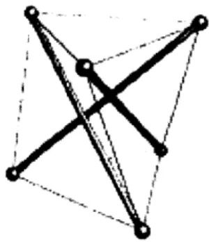
It has been reported that D.G. Emmerich was one of the first to bring attention to the idea of tensegrity structures when speaking of the research carried out by Russian constructivists in the 1920s. (Motro) It is, however, controversial as to who was the precise inventor. Documentation shows that D.G. Emmerich, R. Buckminster Fuller, and Kenneth Snelson all applied for patents for the system around the same time in the 1960s. (Djouadi, Motro and Pons) All three described a system consisting of three compressive struts and nine tensioned cables. This proposed system can be found in Figure 1.1-a.

Figure 1.1-a: Tensegrity system proposed by Emmerich, Fuller, and Snelson (Djouadi, Motro and Pons)

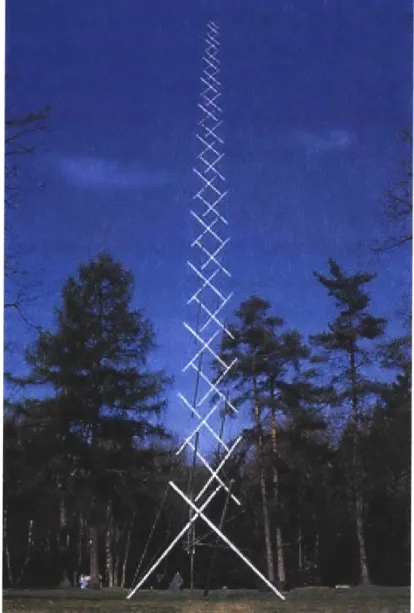
It should be noted that in this system the compressed struts do not join at any point, creating the discontinuous aesthetic described by Fuller. It is debatable whether this characteristic is required in order to fit into the category of tensegrity. As will be discussed later, a formal definition of tensegrity structures excludes systems in which the compressive struts are joined. From this basic system, Snelson produced several sculptures which modeled the concept of tensegrity and what could be accomplished with the assembly of many elements. Images of his "Needle Tower" and "X-shape" can be found in Figure 1.1-b and Figure 1.1-c.

Figure 1.1-b: Kenneth Snelson's "Needle Tower" (University of Cambridge)

Figure 1.1-c: Kenneth Snelson's "X-Shape" (Snelson)

Since their introduction, these systems have proven to be quite advantageous and useful in many applications. Snelson utilized tensegrity mostly towards artistic applications. Tensegrity has, however, been adopted into architecture, robotics, and, as will be discussed further in this paper, structural engineering.

1.1.2 Advantages and Disadvantages

There are several initial draws to tensegrity systems. Since tensegrity structures utilize self-stress to support themselves, they do not require compression rings or any other such anchorage in order to stand. Therefore, they are able to be extremely lightweight. Also as they are constructed only of cables and some compressive struts, they can be very easily assembled and disassembled. A common feature of regular tensegrity systems is to have uniform length for cable and strut members, making fabrication of members extremely simple. In some cases, they can even be made to be foldable and deployable. All these characteristics make tensegrity structures of great use in many applications, particularly in aerospace and ground structures.

---Etienne Fest suggested that applications could include temporary roofs, radio telescopes, and space antennas. (Fest, Shea and Smith)

Given the visual illusion they create of floating members, tensegrity is becoming increasingly popular in architecture. Tensegrity structures are also very flexible and moveable. Since their stiffness comes from the self-stress of the members, their stiffness can be easily adjusted. These attributes make them great candidates, as is the purpose of this paper, for shape change and active control. By using actuators in either the tensioned or compressed members, one can adjust both the shape and stiffness of the system to better meet strength or serviceability requirements.

Though their flexibility is in some ways advantageous, it can also be seen as a downfall. Tensegrity systems can be design to take on heavy loads, however, their flexibility will cause them to deflect considerably even under small loads. This can cause issues of serviceability, depending on the application. Active control can be used to mitigate these deflections and make them more suitable for structural and architectural applications.

1.2 Motivation of Work

This paper will explore the idea of utilizing actuators in tensegrity systems in order to create structures which can adapt to maintain serviceability requirements. The motivation behind this work is twofold. Firstly, it was inspired by the architectural ideal of creating structural forms which interact with their environment. Secondly, active control of tensegrity systems provide a way to minimize deformations, which can be a major downfall of the system in terms of use in structural applications.

1.2.1 Responsive Architecture

Architects and designers have long entertained the idea of "responsive architecture." The idea behind this concept involves structures and architectural elements which interact and adjust based on their environment. In recent years, Tristan d'Estree Sterk has published several papers which discuss this concept. Specific proposals of this idea include walls which move based on

the amount of room space required and building envelopes which expand based on the current programming of the building. A diagram of this concept can be seen in Figure 1.2-a. (Sterk) In his publications, Sterk has identified that the structural systems utilized in such responsive building envelopes must be lightweight, of controllable rigidity, and able to undergo asymmetrical deformations. For this reason, Sterk has suggested the use of tensegrity structures. (Sterk)

A responsive building envelope

and internal partition

4.

A single structural unit

1/ ~ I

3.

2

N

step1. wall senses activity slep2. low-level n1all response triggered step3. well sends an exception when an

obstruction is sensed, high-level processes start step4. high-level request initiates low-level envelope response

Figure 1.2-a: Sterk's model of responsive architecture (Sterk)

While the purpose of this research is not to tailor tensegrity structures to adjustability for architectural applications, responsive architecture is held as inspiration for creating adjustability in structural applications. Instead of creating structures which will be able to create more useful spaces, one can utilize tensegrity and control to create arrangements which will adapt to take on different loadings. This will lead to the design of lighter, more efficient

assemblies. Such a concept could prove extremely popular in building applications, since it utilizes a progressive architectural ideal for functional structural purposes.

1.2.2 Serviceability

As mentioned in the previous section, due to their flexible nature tensegrity structures will undergo large deformations under fairly small loads. This poses a problem for these structures in building applications where serviceability plays a big role. Raja mentioned when introducing his research that "because of their flexible nature... only limited applications of tensegrity structures for practical application are found." (Raja and Narayanan) As this paper will show, however, control can be used to mitigate these deflections. For example, if tensegrity was to be used for a roof where a consistent slope needs to be maintained, active control could be used to maintain such a slope. (Fest, Shea and Smith) By limiting deflections in tensegrity assemblies, they can be more widely applied to building applications.

1.2.3 Problem Statement

This paper will serve to further explore the idea of active control in tensegrity structures. The nature of tensegrity systems and methods of form finding will be discussed in order to give background and highlight its structural applicability. Next, ways by which active control can be integrated into these systems in order to accomplish various design objects will be discussed. The Linear Quadratic Regulator (LQR) algorithm, which can be used to incorporate actuator forces in order to control deflections, will be introduced. Lastly, this algorithm will be applied to a two dimensional tensegrity beam assembly in order to demonstrate the effectiveness of the method. This application will investigate the effects of utilizing varying weighting parameters and actuator force placement in order to draw conclusions with regard to how active control can be efficiently implemented.

2 Physical Systems

2.1 Definition of Tensegrity Structures

With knowledge of the concept of tensegrity in place, Motro provides a concrete definition of true tensegrity structures.

A tensegrity system is a system in a stable self-equilibrated state comprised of a discontinuous set of compressed components inside a continuum of tensioned components. (Motro)

As Motro states, the two major criteria which categorize tensegrity structures are their discontinuous compressed components and their initial stable, balanced state before any external loading, including gravity. In some cases, structures which contain joined compressive elements can be considered tensegrity under an "extended definition." However, for the purposes of this paper, such systems will not be discussed further. Regardless, such a definition provides very stringent requirements as to the geometry of these systems.

The portion of this definition which is most difficult to realize is the self-equilibrated state. To construct these systems, one must determine the topology and stresses which will create such a state. In the case of regular tensegrity structures, this can be accomplished through the identification of a single parameter - the ratio of the length of the cables to the length of the struts. (Djouadi, Motro and Pons) Knowing this parameter and specifying connectivity based on qualitative analysis allows one to construct a regular tensegrity system which will fit its stable criterion. Irregular shapes such as those which have different cable and strut lengths or a double curvature require additional parameters.

Specifying the necessary geometric parameters in tensegrity systems, planar or three-dimensional, requires the employment of form finding. Several commonly used form finding methods, including the one to be used in the later application, will be discussed in the subsequent section.

2.2 Form Finding Methods 2.2.1 Cinematic Approach

For very simple systems which are symmetrical, basic static equilibrium can be used to determine the system's form. This, however, is a very limited approach and in most cases, other methods need to be utilized. In his book, Motro outlines the cinematic approach for form finding, which can be utilized for small scale, regular systems. When determining the appropriate ratio of strut length to cable length, the ratio which will produce a unique and ideal shape is always the largest possible ratio. (Motro) Therefore, if this ratio is defined by a function of some other geometric parameter, the point at which the derivative of that function equals zero will be the ideal ratio.

Motro demonstrates this for a simple three strut cell, shown in Figure 2.2-a.

D D' DI

D

6

Figure 2.2-a: Three-strut cell used to demonstrate cinematic approach (Motro)

Here, the ratio of strut length to cable length can be expressed as a function of the relative angle between the triangles created by the cables, as follows.

s 2 IT

r - [1 + - * sin

0+-c 3 3

Here, s represents the length of the struts, c is the length of the cables, and 0 is the relative angle between the triangles. Since the maximum ratio of r needs to be determined, the derivative of this function can be taken with respect to 0.

d (C N/ ₂₁

=O * - Cos 60+ -*[1 + - * sin ( +--]

d6 33 V- 3

Solving for 0 such that this derived equation equals zero will provide the relative angle at which the ideal ratio is reached. By plugging this value for 0 back into the original equation, r can be determined such that the original equation is satisfied. Once r is known, along with the connectivity between the elements, the topology that will produce the ideal shape can be determined. (Motro)

2.2.2 Dynamic Relaxation

Another method of form finding is dynamic relaxation. As will be shown later on, this method can be incorporated into control in order to find and position a structure into an ideal shape. This method is often used for more irregular and large scale tensegrity systems. The major draw of this method is that it calculates nonlinear behavior directly. This is useful for tensegrity because their inherent large deflections mean that effects of nonlinear behavior need to be taken into account in most cases.

Fest utilized and described this method when speaking of his work in adjustable tensegrity structures. This method utilizes the dynamic equation of a damped system as follows.

p(t)= Md +Cd +Kd

where p(t) is the externally applied load, Mis a fictitious mass matrix, Cis a fictitious damping matrix, Kis a stiffness matrix, and dis a vector associated with the displacement of the system. This method tracks the responses of the nodes of the system over time. When the first two terms in the right side of the equation, associated with the fictitious mass and damping matrices, reach a near zero value, the structure is said to have reached a static position and to

be in a state of stable equilibrium. (Fest, Shea and Smith) The shape of the structure at this point is taken as the optimal shape.

2.2.3 Force Density Method

For larger and more irregular tensegrity structures, the specification of several parameters may be needed to find the ideal shape. For this Vassart developed the force density method, which is discussed by both Motro and Djouadi. For the purposes of this paper, this method will be outlined in detail as described by Motro, since it will be utilized later to specify the initial form of a structure to be controlled to minimize displacements. This method involves the principle of developing force density coefficients for each member as follows.

T

where 19 is the length of the member

j

before loading and T is the axial force in the same member. Equilibrium in terms of a single direction can then be written using these coefficients as follows.

(xi - xh) -q; = fix

In this case, xi and Xh are the position of the two nodes i and h of the member

j

in the x direction. Also,

fix

denotes the external loading in the x direction. Since tensegrity structures must be in a state of equilibrium prior to any external loading,

fi

is zero for this application. The equilibrium condition can be written, in matrix form, to account for all members by the following equation.

CT.Q.C.x= 0

Where C is a b _{x n the branch-node incidence matrix, corresponding to b members and n}

nodes,

Q

is a b x b matrix which is diagonal and comprises the force density coefficients, and x is a vector of the x coordinates of each node. It should be noted here that though these

equations are being written in terms of xcoordinates, the same equations can be used for the y and zdirections.

In the case of structures which are prestressed, the connection matrices would then be split based on those nodes which are "free" and those which are "fixed" in order to imply boundary conditions. This results in the following equation.

CiX T Q. CiX. Xi = -CfXT Q- CfX -xf

where terms corresponding to free nodes are denoted by 1 and those corresponding to fixed nodes are denoted by f

In order to find the form of the structure, one must determine the relations of the elements and specify the connectivity matrices, as well as the force density coefficients. Specifying the force density coefficients is generally the most difficult part of the process. Motro mentions that specifying coefficients such that the rank of the connectivity matrix is n-4 is necessary for solving the form of these systems. The best way to do this for non-simple systems is iteratively or analytically. (Motro) Once the connectivity and force density matrices are known, it is possible to determine the vector of x coordinates (as well as y and z coordinates) and to determine the position of each node. A similar procedure can also be employed in which one specifies desired nodal coordinates and conducts a static equilibrium analysis to obtain the

necessary force densities. This is the strategy which will be employed in the later application. The force density method is straightforward determining the ideal form of an irregular or large scale tensegrity system. Also, it allows one to map these systems to curved surfaces in order to

create more interesting and applicable structures. (Djouadi, Motro and Pons)

2.3 Elementary Cells and Assemblies

The simplest form of a tensegrity structure is known as a "cell." Elementary cells are often described as the "atoms" of a tensegrity system since they cannot be broken down into smaller tensegrity systems. (Motro) These small tensegrity cells are useful, as they are a known

arrangement which can be built up to create larger systems. Two different types of elementary cells are shown below in Figure 2.3-a and Figure 2.3-b.

Figure 2.3-a: Simplex (elementary cell) (Motro)

Figure 2.3-b: Expanded Octahedron (elementary cell) (Motro)

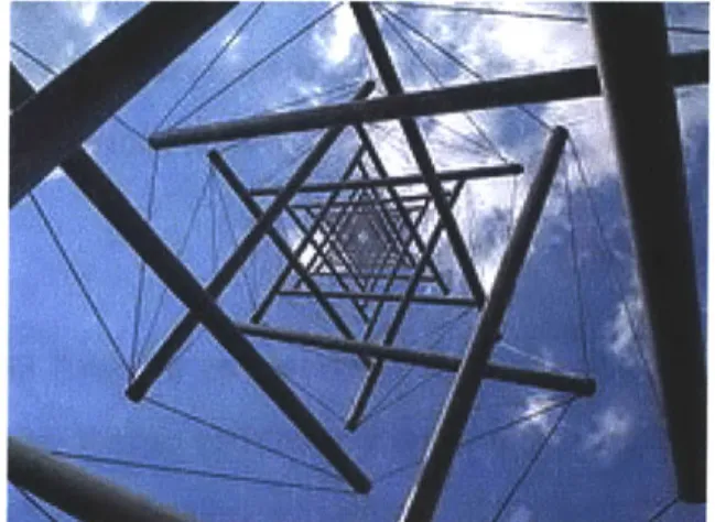
The top figure shows a "simplex," which is a three-strut system connected by nine cables. The other, an "expanded octahedron" is a six-strut system joined by eighteen cables. These cells are often assembled together to create larger structures. For example, Kenneth Snelson's Needle Tower can be viewed as a superposition of expanded octahedron cells. This is made clear when looking at a bottom view of the tower, as shown in Figure 2.3-c.

Figure 2.3-c: View from bottom of Snelson's "Needle Tower" (Wikipedia)

Expanded octahedrons were also used to create a tensegrity arch, as shown in Figure 2.3-d.

Figure 2.3-d: Tensegrity arch (Motro)

For the purposes of the application in this paper, an assembly of two-dimensional cells will be used to create a tensegrity beam. An example of such a cell can be found in Figure 2.3-e.

Figure 2.3-e: Two-dimensional tensegrity cell (Skelton)

It should be noted that here the red lines represent struts and the black lines represent cables. For the assembly to be used in this simulation, each cell will consist of two struts and six cables. As will be discussed in the next chapter, this system is similar to the system used in van de Wijdeven's research. An example of the three-cell system assembled in this fashion, as was used by van de Wijdeven, can be found in Figure 2.3-f.

6 4 10 a 12

1.25 M

15 3 9 7 1

x

Figure 2.3-f: Two-dimensional cell assembly as used in Wijdeven's work (van de Wijdeven and de Jager)

Specifying such an assembly allows for the determination of member connectivity, which will prove useful in identifying the form of the system used in the control problem.

3 Control Algorithms

3.1 Types of Control Objectives

Now that a background of tensegrity structures has been given, along with a description of how their shapes are found, an overview of recent research in tensegrity control will be presented. Tensegrity control research has utilized a variety of methods to accomplish various control objectives, depending on the context of the problem. These different control objectives and methods, along with their applicability to structural engineering applications, will be discussed. The simulation presented later on in this paper will utilize the LQR algorithm in order to maintain deflections in a two-dimensional tensegrity beam under dynamic loads. For this reason, this method will be discussed in further detail here.

3.1.1 Maintaining Shapes

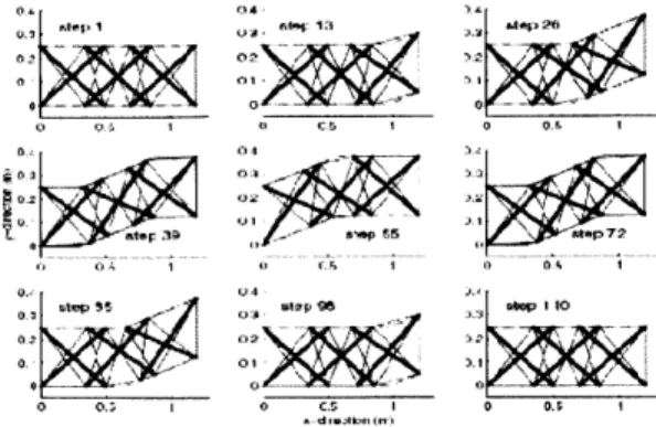
Jeroen van de Wijdeven, in his work with tensegrity control, discussed utilizing control in order to maintain shapes in moveable structures. He proposed a tensegrity beam that would move according to some user specified trajectory. This trajectory would be broken up into steps of "sub-movements," which were determined such that the step fit with the desired shape, as well as minimized forces in the members. (van de Wijdeven and de Jager) An image of the model van de Wijdeven used to conduct this procedure was already presented in Section 2.3. Given this model, an example of van de Wijdeven's various "sub-movements" is show in Figure 3.1-a.

04

-0 0 0 0 05 I

Figure 3.1-a: van de Wijdeven's shape change sub-steps (van de Wijdeven and de lager)

Control devices would be used to transform the structure into the desired shape, but more importantly would serve to mitigate vibrations during shape change such that the specified shape would be constantly preserved. Since tensegrity structures have little damping, vibrations needed to be mitigated using feedback control in addition to the feedforward control used for the shape change. (van de Wijdeven and de Jager) Though this type of control is not examined further here, as it is outside the scope of this paper, this type of control can have many structural applications. For example, this may serve useful in the design of retractable or deployable tensegrity roof structures. Also, this idea of a user-defined shape trajectory relates well to the idea of creating responsive architecture which adapts based on what is most useful for the user.

The work of Etienne Fest and Bernard Adam also focused on using control to maintain shapes on portions of tensegrity assemblies. Fest's work involved utilizing form finding and search methods, which will be discussed in Section 3.2, to maintain the slope of a tensegrity roof under static loads. (E. Fest, K. Shea and B. Domer) A diagram of the studied tensegrity structure, along with the area at which the slope was maintained can be found in Figure 3.1-b and Figure 3.1-c.

Ars ofO~eModule 4 Mode 5

Z 50 39 _. .. ... _JA PL\ -.- ~-PH __M~i!I~k T --- --- V 37 41 45

Cable in plane --- Cabl out of plano StPa

SLoaded joint

+

Dimiacent Acluor D Skope refeence points Figure 3.1-b: Fest's tensegrity roof

(Fest, Shea and Smith)

Am dahs- -mmdamnsa

/L

5

1

-. cs in vAiv _{Module 3} - Cabe uo sepine 3 - - -

-+

ngp-s 1mento

N 1 bao unaene d wa samd

Figure 3.1-c: Area of slope maintenance (Fest, Shea and Smith)

Adam's work expanded on this problem through the use of a multi-objective search method which not only maintained a consistent roof slope, but also minimized the forces in the members under various static loads. (Adam, Smith and ASCE) Both these works demonstrate the possibility of utilizing control to maintain relationships between nodal points. This could prove to be extremely applicable in building structures. For example, slopes may need to be maintained in order to facilitate drainage or preserve clearances.

3.1.2 Controlling Deflections

One of the most popular objectives in the control of tensegrity structures is minimizing deflections. As mentioned previously, tensegrity structures are inherently flexible and thus, serviceability can be a major problem. The works of M. Ganesh Raja and S. Djouadi both serve to demonstrate the use of control toward this objective. In the work of Raja, optimal control theory is used to minimize deflections in a small scale structure when subjected to random excitation at a single node. (Raja and Narayanan) Raja runs several simulations with various

27

levels of control to develop a relationship between the amount of control that can be accomplished versus the amount of voltage and control effort required.

Djouadi's work also served to minimize deflections, this time in a tensegrity beam, due to random excitations. Here, instantaneous optimal control was used along with a varying number of actuators in order to evaluate different levels of performance compared with amount of control effort. (Djouadi, Motro and Pons) Between Djouadi and Raja, a theme can be seen in balancing the amount of control desired with the amount of control effort needed. This is an important component of control, as the energy required to control a system can be very expensive. Being able to obtain enough deflection control without an excessive amount of effort or actuated members is extremely important in making these assemblies feasible in actual structures.

The simulation to be conducted later on in this paper will expand upon this control objective. Djouadi and Raja's works focused on comparing numbers of actuators and types of H controllers, respectively. In this simulation, however, variations in LQR weighting matrices and

locations of the actuators, particularly on cable versus strut elements, will be the main points of comparison.

3.1.3 Optimization

One control objective which is touched upon in the works of Adam, Raja, and Milenko Masic is the idea of utilizing control for structure optimization. As mentioned, in Adam's work an algorithm is developed which is intended to satisfy multiple objectives including minimizing stresses in the elements. (Adam, Smith and ASCE) His model predicts the behavior of the structure and then serves to optimize the shape accordingly. In a different way, Raja also aimed to simultaneously optimize and control his structure. Here, Raja identified a single shape parameter, in this case the "twist angle" of the structure, which is to be optimized such that the amount of control can be minimized. A diagram showing this studied structure and the corresponding "twist angle" can be found in Figure 3.1-d.

Excitation

Module I Actuator

W U

Figure 3.1-d: Raja's structure and "twist angle" (Raja and Narayanan)

Similar to Raja's work, Masic also sought to optimize the structure through an initial selection of parameters. His work served to select prestress forces for the members such that the LQR control output could be optimized. (Masic and Skelton) All these works aim to create simultaneous control and optimization of a tensegrity structure. This is useful as it demonstrates how deflections and vibrations can be mitigated, while at the same time adjustment of structure shape can be utilized to minimize the amount of control necessary. Control, as mentioned, can be expensive and so this type of optimization can prove to make control of tensegrity structures much more feasible. While time constraints and program capability are such that optimization is out of the scope of this particular paper, it is recommended that such optimization should be considered in further extensions of this research.

3.2 Review of Developed Methods

A variety of methods have been developed by which these control objectives can be

accomplished. A review of these methods and an evaluation of their usefulness will be discussed in the following sections.

3.2.1 Search Methods

When controlling a structure to maintain a certain slope at a specified point, Fest and Adam utilized a stochastic search algorithm. Such an algorithm is based on the assumption that

29

"better sets of solutions are more likely to be found in the neighborhood of sets of good ones." (Fest, Shea and Smith) Thus, this algorithm searches for solutions based on the probability density function. A schematic diagram of this algorithm can be found in Figure 3.2-a.

Load

YO _Yn

YO: initial state Y're adjstrent aray

Ui:

vttuotrW

response

L Ivm ]

Yn = Y, for inft loop

YnwXY,, Yn) for a4u~tmsihs( V sr: n*O)

Figure 3.2-a: Shape control methodology by Fest (Fest, Shea and Smith)

Here, the structure is subjected to a static loading and the response of the structure is sensed. This response is inputted into the search algorithm. Here, the continued response of the structure is predicted using dynamic relaxation, a form finding method as discussed in Section 2.2.2. This method was chosen due to its ease of incorporating nonlinear behavior. With the predictive model of the structure in place, the search outputs a series of strut elongations such that the slope of the roof can be maintained, keeping in mind constraints such as the elastic limit of the cables. (Fest, Shea and Smith) The search involved a very complex process of evaluating every possible shape configuration. In order to decrease the size of the solution space, Fest limited the number of adjustable bars used and the range of motion each of these bars would have. This method was applied to a physical model and proved successful in predicting responses and adjusting shapes based on these responses.

Adam's work sought to expand upon the algorithm developed by Fest. In his work, the same structure and static-type loading is used. Here, however, Adam applies multiple objectives as the goals of the search. The objectives are as follows:

e Slope: maintain top surface slope of the structure when subjected to loading

* Stroke: maintain actuator jacks as close as possible to their midpoint * Stress: minimize stress of the most stressed element

* Stiffness: maximize the stiffness of the structure

(Adam, Smith and ASCE)

Adam utilizes a ParetoPGSL algorithm in order to determine the ideal shape change. This process identifies an optimal solution set based on the criteria listed above and then selects the most optimal solution from that solution set. A schematic diagram of this process can be found in Figure 3.2-b.

Structure and Load Case

Pareto Optimal Solutions

ParetoPGSL

Slope Stroke Stress Stiffness

Hierarchical Selection

1) Reject solutions with less than 95% of Slope compensation,

2) Reject the worst third for stroke,

3) Reject the worst half for stress,

4) Identify the best solution for stiffness.

(Control Command

Figure 3.2-b: Adam's multi-objective methodology (Adam, Smith and ASCE)

As shown, Adam takes the four objectives and ranks them such that solutions can be eliminated based on their compliance with each of the objectives. From his results, Adam determines that

this type of approach produces robust results and more efficient control than in a single objective search. (Adam, Smith and ASCE)

Adam and Fest's work show that search algorithms, in particular those that use multiple objectives, can be made very useful, as they will produce shape changes to provide more efficient tensegrity structures based on loading. These methods may, however, have some downfalls. Firstly, though Adam's model did eliminate some solutions which required much control effort and amount of control effort was thus decreased, minimal information was given as to how much control effort would still be needed. This would need to be evaluated in order to determine how feasible such a scheme would be. Also, these models demonstrated such an algorithm with respect to static loading and minimal information was given as to the run time of the search and shape change. This aspect would need to be evaluated when applying to this method to more realistic structures where dynamic loads exist and the required shape change would be more rapidly changing.

3.2.2 H Controllers

One of the downfalls of the search methods described above was the lack of focus on control effort. The work of Raja and van de Wijdeven employed the use of optimal control, particularly H2 and H. controller norms, to choose control parameters such that the performance index of the controllers are minimized. To describe this method, a diagram of the closed loop system used for this type of control is shown in Figure 3.2-c.

Figure 3.2-c: Raja's closed loop system (Raja and Narayanan)

Here, w(s) represents the inputs to the system, such as any disturbances. The regulated output is represented by z(s), the sensed output by y(s) and the actuator input by u(s). G(s)

represents the transfer function produced by the structure. That is, it represents the function which relates the inputs of the system to the structural response. K(s) represents the transfer function which relates the sensed outputs to the desired force produced by the actuator. (Raja and Narayanan) Optimal control theory seeks to find a controller, or function K(s), which "stabilizes" G(s), or rather effectively controls response, while minimizing the performance index. The works of Raja and van de Wijdeven collectively utilized both H2 and Hmcontroller

norms, which define the performance index in two different ways. The Hz normal characterizes the performance index as

J2(K) =

IIF(G,

K)||1

where

J2(K) = z(t)Tz(t)dt

k=1

It should be noted that here, z(t), relates to the observed output from the state space. This aspect will be discussed further in the next section, as it relates to the linear quadratic regulator

algorithm. The H. norm identifies the performance index as

J. (K) = |IF(G,K)I|

where

Jc(K) = sup

{

: w # 0

Further details as to how the state space is used to satisfy these performance indices can be found in Raja's works. (Raja and Narayanan) The work of van de Wijdeven also applies the method of H₂norms, although it is there described in less detail.

H2 and H. controller norms, in both these applications, proved to be successful in controlling

deflections. This method is also useful in that it takes into account the control effort of the system and seeks to minimize this parameter. For this reason, a variation of the method used here, the linear quadratic regulator, will be utilized in this paper's simulation.

3.2.3 Linear Quadratic Regulator (LQR)

The LQR algorithm has been used in some previous works. For example, as mentioned, Masic used LQR control to choose prestress forces which would create the most control for the least effort. (Masic and Skelton) A description of this algorithm can be found in Jerome Connor's textbook, Introduction to Structural Motion Control. A variation of the H2 control mentioned in

the previous section, LQR seeks to limit the performance index of the controllers. It does this by utilizing the state space, as well as designer specified weighting matrices. The state space of a system can be described as follows:

X = AX + BU Y = CX + DU

Here, Xis considered to be the state vector of the system, Uis the input or control vector, A is a matrix representing the system, Bis a matrix representing the inputs, Cis the output matrix, and Dis "feedthrough" matrix. Yis considered to be the "output" vector.

When using the LQR algorithm, the performance index is defined as follows:

S= u[qa U2 + qt + r(kdu + k, fu) 2] dt

Written in matrix form, this equation takes on the following form.

] = fXT(Q + K] RKf)XT dt

As can be seen, the performance index relates to X, which as mentioned is the state vector of the system. The

Q

and R matrices are diagonal weighting matrices that are determined by the designer. The matrix

Q

relates to the importance of control and R relates to the importance of

34

preserving cost, or controller force. These are specified based on what the designer deems to be the priority, control or cost. The matrix Kf relates to the gain that the system will see from the controller. Based on the matrices X,

Q,

and R, the LQR algorithm seeks to find an optimal K

such that the index

fis

minimized.

To solve this optimization problem, Jis written as a Liapunov function as follows.

d

xT(Q+ KjRKf)XT= _{f f} dt(XTHX)

dt

This equation is expanded to the following.

d

(XTHX) = XT(AcH + HAc)X

dt

Here, Ac refers to the revised A matrix in the state space equations. The right side of the side of the equation can then be substituted into the performance index equation, which reduces the integral to the following equation.

1

J = -XT (O)HX(O)

2

Here, it is necessary to require that Jbe stationary with respect to Kr, which allows one to set the condition of dH = 0. Manipulating these equations and utilizing this condition provides the

following equation for the optimal K:

Kfoptimat = R-1_{BT H}

Similarly, the matrix Hcan be found by solving the following equation.

AT H + HA - HBfR- 1BTH = -Q

where His a positive definite matrix. (Connor)

This algorithm provides a simple procedure for determining optimal control. It does, however, have a few limitations. First, LQR utilizes a full state feedback. That is, the displacement and velocity at every node is known. While this works in the theoretical realm, in real structures this

is not realistic. Methods for control based on only a few feedback points have been developed, however, such methods are out of the scope of this paper. The simulation to follow will utilize LQR and full state feedback, though this drawback should be kept in mind.

Another limitation, as it relates to this application, is the issue of nonlinearity. Tensegrity systems are susceptible to large deformations and thus, nonlinear behavior usually should be taken into account. LQR, as it utilizes only one iteration to compute system gain, relates to linear behavior, which may lead to inaccuracies in results. LQR could account for nonlinear behavior by altering the Ac matrix continuously to account for the change in stiffness and therefore continuously recalculating the optimal gain. However, due to limitations in programming this was not utilized. The application to follow will not take nonlinearity into account when determining the stiffness of the system and optimal control gain. Though this may lead to some inaccuracies, it is thought that since the control will be limiting deflections, nonlinear behavior will be minimal. This, however, should be verified in further research and ways to incorporate nonlinearity should be developed.

4 Control Application: Two-Dimensional

Tensegrity Beam

4.1

Overview

The following application will demonstrate how active control, whose gain is optimized by the LQR algorithm, can be utilized to limit deflections in a tensegrity structure. The system studied will be a planar beam that is simply supported. This system was chosen, given its potential real world applications. For instance, simply supported tensegrity spans could be used in pedestrian bridges. An example of such an arrangement is shown in Figure 4.1-a.

Figure 4.1-a: Tensegrity pedestrian bridge in Brisbane, Queensland (Sustainable Design Update)

The two-dimensional tensegrity beam will not be regular in the sense that all cable and strut lengths will be respectively the same. However, it will still be simple in layout. The force density method, utilizing some intuitive assumptions, will be used to determine the initial coordinates

37

of the nodes and prestress forces in the members. Then, the system will be subjected to a harmonic force in the vertical direction at every node. Actuator forces will be placed on nodes associated with the outer and inner struts and cables separately in order to limit the deflection towards the mid span. LQR will be used to determine the amount of control gain to be used, based on several different specified

Q

and R matrices. The level of control compared to the control effort will be examine for the different weighting matrices and different actuator placements in order to draw comparisons and conclusions with regard to efficiency and effectiveness.

4.2 Tensegrity System Formulation

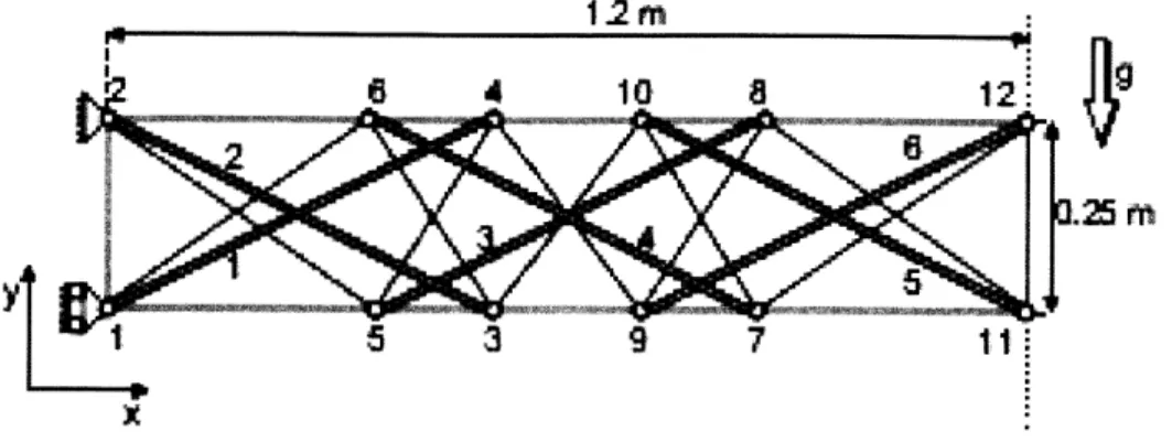
The tensegrity beam arrangement to be used was based upon the model utilized in van de Wijdeven's work, as was shown in Figure 2.3-f. Similarly, the model used in this application consists of ten struts, arranged as five "X" shapes linked by 38 tension cables. The ends of this beam are pin connected at the bottom and roller connected at the top. An image of this arrangement is shown Figure 4.2-a.

() Node Number 10!] Element Number N Compression Strut * Tension Cable (1) 33 57 1 1 11331] 137

Figure 4.2-a: Model and numbering strategy

As can be seen, the 48 members are connected to 20 nodes. Each node has two degrees of freedom - translation in the horizontal and vertical direction. The numbering strategy for the

38

numbers and element are also shown in the image above. Table 4.2-a outlines the connectivity for this system.

Element Node 1 Node 2

1 1 2 2 1 3 3 1 4 4 2 3 5 2 4 6 3 5 7 3 6 8 4 5 9 4 6 10 5 7 11 5 8 12 6 7 13 6 8 14 7 9 15 7 10 16 8 9 17 8 10 18 9 11 19 9 12 20 10 11 21 10 12 22 11 13 23 11 14 24 12 13

Element Node 1 Node 2

25 12 14 26 13 15 27 13 16 28 14 15 29 14 16 30 15 17 31 15 18 32 16 17 33 16 18 34 17 19 35 17 20 36 18 19 37 18 20 38 19 20 39 1 6 40 2 5 41 3 10 42 4 9 43 7 14 44 8 13 45 11 18 46 12 17 47 15 20 48 16 19 This connectivity assembly. will be used

Table 4.2-a: Element connectivity

in both the force density method and the stiffness matrix

4.2.1 Determining Geometric and Material Properties

The initial coordinates of and pretension forces in each member were determined using the force density method. As can be recalled from Section 2.2.3, the fundamental equations used in this method are as follows.

CiX T-

Q

-

CiXx

=

0

CiyT.

Q-

Ciy -yi = 0

It should be noted that in these equations, the right side is set to zero as opposed to the force density of the fixed nodes. In order to ensure a true, self-supported tensegrity system, the coordinates and force densities were determined assuming no pin or roller supports. The degrees of freedom associated with these connected nodes will be eliminated from the global stiffness matrix after it is assembled to model the fixity at those nodes.

Referring back to the previously listed equations, the C1 matrix is the branch-node incidence matrix that is associated with the connectivity according to Table 4.2-a. In this matrix, for each row m associated with the member m, -1 is placed in column a, associated with the first node

of the member, and 1 is placed in column b, associated with The produced C1matrix is shown, in abbreviated form, below.

C, =

the second node of the member.

As each node holds a translational degree of freedom for both the x matrix is the same in both directions. The

Q

is a diagonal matrix of the each member, which is also the same for both directions.

and y direction, the C, force density terms for

For the purposes of this application, the desired xand ycoordinates were chosen such that a regular geometry could be maintained. Table 4.2-b identifies the desired x and y coordinates of each node.

Node 1 2 3 4 5 6 7 8 9 10 11 12 13 14 15 16 17 18 19 20

X - Coord 0 0 12 12 20 20 24 24 32 32 36 36 44 44 48 48 56 56 68 68

Y-Coord 10 0 10 0 10 0 10 0 10 0 10 0 10 0 10 0 10 0 10 0

Table 4.2-b: Nodal coordinates

Using these set coordinates, the force density terms can be determined such that the fundamental equations are satisfied. There is, however, more unknown force densities than equations, so some assumptions need to be made based on intuition. For this, it is first assumed that the vertical tension cables will have the same force density. This is also assumed for the outer horizontal cables, outer angled cables, inner horizontal cables, inner angled cables, outer struts, and inner struts. Figure 4.2-b depicts these force density assumptions. Members shown in like colors are thought to have equivalent force densities.

3 500911

9 13 17-142 2963

4 6 8 1011@61

Figure 4.2-b: Color representation of force density assumptions

Given these assumptions, the force densities of each member can be determined. The geometric and material properties were also assigned reasonably estimated values. The material used was assumed to be steel for both cables and struts. The cross sectional areas were chosen such that the strut would not buckle under its initial prestress load and such that the cable is roughly one tenth the area of the strut. A summary of the force densities and material properties of each member can be found in Table 4.2-c. It should be noted that in this table the elements are sorted into categories in the same way as show in Figure 4.2-b.

Force Initial Diameter Area Length Modulus of

Element Type Density Force Elasticity

(kips/in) (kips) (in) (in2) (ft) (ksi)

Vertical Cables 1 120.000 10.0000

Outer Horizontal Cables 2.333 336.000 12.0000

Outer Diagonal Cables 187.500 3.000 15.6250

Inner Shorter Diagonal Cables 1 129.244 7.065 10.7703

29000

Inner Longer Diagonal Cables 153.674 12.8062

Inner Shorter Horizontal Cables 432.000 4.0000

9

Inner Longer Horizontal Cables 864.000 10.000 8.0000

Struts -2 -536.657 78.500 22.3607

Figure 4.2-c: Summary of member properties

These properties can then be used to formulate the stiffness and damping of the system, as identified in the next section.

4.2.2 System Properties Formulation

In order to conduct a dynamic analysis of the system, it is necessary to identify the mass, damping, and stiffness matrices of the system. With regard to the mass matrix, the mass of the tensegrity system itself is assumed to be massless. An arbitrary lumped mass of 10 kips is placed at each node. Therefore, the mass matrix is a diagonal matrix of 10 kips. The damping of the system is thought to be relatively small and proportional to the elastic component of the stiffness matrix. The damping matrix is defined by the following equation.

C = 0.003* K

where Kis the stiffness matrix.

Lastly, the stiffness matrix needs to be defined. In a tensegrity system, there exist three components of the stiffness matrix. These are as follows.

K1ocal = KL + KNL + KS

Here, KL refers to the classic linear stiffness matrix, KNL refers to the stiffness which takes into account nonlinearity, and K refers to the initial stresses matrix, or geometric stiffness. (Motro) For a given local element, each of these components is defined as follows.

1 0 -1

0-K = - -1

0 -1 0 101

(Au-L)2 (Au-L)-Av -(Au-L) 2 -(Au-L)-Av

K _NL(Au-L)Av

A

(Au - L) -AV Av2 -(Au - L) -Av -AV2

(Au-L)2

(Au - L) AV

(Au-L)-Av -AV2 (Au-L)-Av Av2

1 0 -1 0~

Ks =qo j -1

s 1 0 1 0

0 -1 0 1.

Here, E, A, and L are the material properties defined in Section 4.2.2 and qo is the specified force density of the given member. The Auand Avterms are given by the following equations.

Au = U1 - U₂

Av = V1 - V2

where ul, u2, vi, and v2are the displacements of the first and second nodes in the xand y

directions. It should, however, be noted that due to programming constraints, the nonlinear component of the stiffness was not taken into account in this application. Thus, the local member stiffness reduces to the following equation.

Klocal = KL + KS

With the local stiffness matrices for each member identified, the global stiffness matrix can be defined as the summation of the member stiffnesses in the global reference frame.

m

Kglobal = Kilobal

i=1

The global member stiffness can be defined from the local member stiffness from the following transformation.

Klocal = L (R - KLoca R )-L

The matrices Rand L _{are the rotation matrix from the local to global reference frame and the}

Boolean connectivity matrix, respectively. With the stiffness, damping, and mass matrices in place, the system is fully defined and dynamic analysis can be conducted.

4.2.3 Control Parameters

To optimize the control force on this system, the linear quadratic regulator algorithm will be used. As discussed in Section 3.2.3, this requires specifying weighting matrices,

Q

and R. To view the results of placing more weight on controlling the deflection or minimizing the control force, three different sets of Qand R matrices will be specified. These are as follows.

1 0 --- 0~

1 0 -- 0

100

0

-.

0 1

0 00 00 100 ... 0 0 0 --- 1. 0 0 0-1 0 0 --- 100 1 0 --- 0~ 100 0 ... 0 1 0 -- 0

0 1 -- 0

0 100

...

01

0

1

.-

0

0 0 --- 1. 0 0 .- 100] 0 0 _--

1-To evaluate the optimal gain, the LQR function in MATLAB will be utilized. This function, given the A and B parameters of the state space and the specified weighting matrices, R and

Q,

gives the optimal gain K. _{An example of such a gain matrix, in abbreviated form, for the case of}

actuator placement at all nodes and weighting matrices R1 and

Q

1, is shown below.