Integrating fossils, phylogenies, and niche models into biogeography to reveal ancient evolutionary history: the case of hypericum (hypericaceae)

(1)

HAL Id: hal-02638449

https://hal.inrae.fr/hal-02638449

Submitted on 28 May 2020

HAL is a multi-disciplinary open access

archive for the deposit and dissemination of

sci-entific research documents, whether they are

pub-lished or not. The documents may come from

teaching and research institutions in France or

abroad, or from public or private research centers.

L’archive ouverte pluridisciplinaire HAL, est

destinée au dépôt et à la diffusion de documents

scientifiques de niveau recherche, publiés ou non,

émanant des établissements d’enseignement et de

recherche français ou étrangers, des laboratoires

publics ou privés.

biogeography to reveal ancient evolutionary history: the

case of hypericum (hypericaceae)

Andrea Sanchez Meseguer, Jorge M. Lobo, Richard Ree, David J. Beerling,

Isabel Sanmartin

To cite this version:

Andrea Sanchez Meseguer, Jorge M. Lobo, Richard Ree, David J. Beerling, Isabel Sanmartin.

Inte-grating fossils, phylogenies, and niche models into biogeography to reveal ancient evolutionary history:

the case of hypericum (hypericaceae). Systematic Biology, Oxford University Press (OUP), 2015, 64

(2), pp.215 - 232. �10.1093/sysbio/syu088�. �hal-02638449�

(2)

non-commercial re-use, distribution, and reproduction in any medium, provided the original work is properly cited. For commercial re-use, please contact journals.permissions@oup.com DOI:10.1093/sysbio/syu088

Advance Access publication November 13, 2014

Integrating Fossils, Phylogenies, and Niche Models into Biogeography to Reveal Ancient

Evolutionary History: The Case of

Hypericum (Hypericaceae)

ANDREAS. MESEGUER1,2,∗, JORGEM. LOBO3, RICHARDREE4, DAVIDJ. BEERLING5,ANDISABELSANMARTÍN1

1_{Department of Biodiversity and Conservation, Real Jardín Botánico, CSIC, Plaza de Murillo 2, 28014 Madrid, Spain;}2_{INRA, UMR 1062 CBGP Campus}

International de Baillarguet, 34988 Montferrier-sur-Lez, France;3_{Department of Biogeography and Global Change, Museo Nacional Ciencias}

Naturales-CSIC, 28006 Madrid, Spain;4_{Department of Botany, Field Museum of Natural History, Chicago, IL 60605, USA and}5_{Department of Animal}

and Plant Sciences, University of Shefﬁeld, Shefﬁeld S10 2TN, UK

∗_{Correspondence to be sent to: Department of Biodiversity and Conservation, Real Jardín Botánico, CSIC, Plaza de Murillo 2, 28014 Madrid, Spain;}

E-mail: asanchezmeseguer@gmail.com and isanmartin@rjb.csic.es Received 31 January 2014; reviews returned 27 May 2014; accepted 7 November 2014

Associate Editor: Austin Mast

Abstract.—In disciplines such as macroevolution that are not amenable to experimentation, scientists usually rely on current observations to test hypotheses about historical events, assuming that “the present is the key to the past.” Biogeographers, for example, used this assumption to reconstruct ancestral ranges from the distribution of extant species. Yet, under scenarios of high extinction rates, the biodiversity we observe today might not be representative of the historical diversity and this could result in incorrect biogeographic reconstructions. Here, we introduce a new approach to incorporate into biogeographic inference the temporal, spatial, and environmental information provided by the fossil record, as a direct evidence of the extinct biodiversity fraction. First, inferences of ancestral ranges for those nodes in the phylogeny calibrated with the fossil record are constrained to include the geographic distribution of the fossil. Second, we use fossil distribution and past climate data to reconstruct the climatic preferences and potential distribution of ancestral lineages over time, and use this information to build a biogeographic model that takes into account “ecological connectivity” through time. To show the power of this approach, we reconstruct the biogeographic history of the large angiosperm genus Hypericum, which has a fossil record extending back to the Early Cenozoic. Unlike previous reconstructions based on extant species distributions, our results reveal that Hypericum stem lineages were already distributed in the Holarctic before diversiﬁcation of its crown-group, and that the geographic distribution of the genus has been relatively stable throughout the climatic oscillations of the Cenozoic. Geographical movement was mediated by the existence of climatic corridors, like Beringia, whereas the equatorial tropical belt acted as a climatic barrier, preventing Hypericum lineages to reach the southern temperate regions. Our study shows that an integrative approach to historical biogeography—that combines sources of evidence as diverse as paleontology, ecology, and phylogenetics—could help us obtain more accurate reconstructions of ancient evolutionary history. It also reveals the confounding effect different rates of extinction across regions have in biogeography, sometimes leading to ancestral areas being erroneously inferred as recent colonization events. [Biogeography; Cenozoic climate change; environmental niche modeling; extinction; fossils; Hypericum; phylogenetics.]

In historical biological disciplines such as

macroevolution or macroecology, which are not in general amenable to experimentation, scientists need to rely on present-day observations to make inferences about the past. For example, systematists use current variation in morphological and/or DNA traits to reconstruct phylogenetic relationships and rates of nucleotide mutation. In historical biogeography, biogeographers use phylogenetic relationships and present distribution data to infer ancestral geographic

ranges and past biogeographic events (Lomolino et al.

2010). Assuming that “the present is the key to the past”

(and the future) is to a certain extent inevitable in a comparative observational science that deals with scales of space and time at which experimental manipulation is

hardly possible (Lomolino et al. 2010). This assumption

permeates methods in biogeographic inference. For example, it is the basis for the assignment of cost values in event-based biogeographic methods, in which processes such dispersal and extinction are penalized (higher cost) because they partly erase previous distributional history—preventing the recovery of “phylogenetically conserved” distribution patterns—, whereas vicariance and within-area speciation are given a low cost because they involve inheritance of distributional ranges

(Ronquist and Sanmartín 2011). Similarly, in parametric methods such as dispersal–extinction–cladogenesis (DEC), ancestral ranges are inferred conditional on the distribution of the extant descendants; however, correct estimates can only be obtained if extinction and dispersal rates—which are modeled as stochastic processes evolving along branches—are low in relation

to cladogenesis (Ree and Smith 2008).

One scenario that is particularly damaging to the assumption that the present is the key to the past is when extinction rates are so high that the biodiversity we observe today is no longer representative of the historical diversity. Extinction erases the evidence of past speciation events and, as we move back into the past, there is less information to infer ancestral states. This results in inferences for basal cladogenetic events that are often uncertain and tend to include a large

number of areas (Ronquist and Sanmartín 2011), or

even wrong biogeographic reconstructions if extinction

has been particularly high within an area (Lieberman

2005). A possible solution comes from the fossil

record, which provides direct evidence on the extinct biodiversity fraction that we cannot observe. So far, the use of fossils in biogeography has been limited to the provision of calibration points for phylogenetic dating 215

at INRA Institut National de la Recherche Agronomique on September 11, 2015

http://sysbio.oxfordjournals.org/

(3)

(Ho and Phillips 2009). However, recent biogeographic studies have shown that incorporating the geographic distribution of fossils to the analysis may change

dramatically the inferred biogeographic scenario (Mao

et al. 2012; Nauheimer et al. 2012; Wood et al. 2012). These studies, however, have relied on using fossils as additional lineages in the phylogeny, which requires coding the morphological traits of the fossil taxa

alongside the extant molecular characters (e.g.,Mao et al.

2012), or assuming arbitrary branch lengths for the fossil

lineage (Nauheimer et al. 2012).

In addition to the temporal and spatial aspect, fossils can provide information on the climatic preferences of ancestral lineages, that is, the environmental conditions in which they reproduced and maintained viable populations, which may then be used to

reconstruct past geographic ranges (Sanmartín 2012;

Stigall 2012). Surprisingly, biogeographers have been slow to incorporate ecological information to their biogeographic models. For example, it has become common practice in parametric biogeography to include information on the past conﬁguration of areas in the time-dependent transition matrix that governs the

movement between geographic states (Buerki et al. 2011;

Mao et al. 2012). Dispersal rates are scaled to reﬂect the presence of a temporal land bridge, increasing the probability of movement between two regions (e.g., the Beringian Bridge between Asia and North America). However, land dispersal is probably as much conditioned by the presence of a physical bridge as by the existence of climatic conditions along the bridge that are within the ecological limits of the dispersing

organism (Sanmartín et al. 2001;Wiens and Donoghue

2004). For example, limiting climatic tolerances might

be behind some global biodiversity patterns such as the Latitudinal Diversity Gradient: the excess of plant species in tropical regions compared with temperate latitudes has been explained by the greater climatic stability of these regions over time, and the inability of many lineages that originated in tropical conditions to evolve the relevant adaptations required to move into

the seasonal temperate climates (Wiens and Donoghue

2004;Donoghue 2008).

Environmental niche modeling (ENM) techniques in combination with phylogenetic evidence offer one way to approximate the climatic preferences of lineages and thus identify potential evolutionary changes in climatic tolerances or detect areas that were climatically adequate

in the past (e.g., Yesson and Culham 2006; Smith and

Donoghue 2010). These studies, however, are limited by the fact that they are based exclusively on present-day distributions and assume to some extent that ancestral lineages shared the same climatic requirements as their extant descendants. Although this might be true for short time scales, it becomes less likely over geological

time scales of millions of years (Peterson 2011; Stigall

2012). To break this assumption, some paleoecologists

have used ENM models based on fossil distributions to trace the evolution of climatic preferences over longer

time scales (Stigall Rode and Lieberman 2005; Stigall

2012). But the incompleteness of the fossil record and

the lack of environmental data in the deep past have so far limited this approach to recent geological periods (Nogués-Bravo et al. 2008) and small geographical

regions (Maguire and Stigall 2009).

Here, we introduce a new approach to incorporate into biogeographic inference the temporal, spatial, and climatic information provided by the fossil record as direct evidence of the extinct biodiversity fraction. First, the spatial range of a fossil is used to constrain the inference of ancestral areas for the node to which that fossil is assigned, thus obviating the need to include it as an additional lineage in the phylogenetic analysis. Second, we use ENM techniques based on fossil and extant distribution data and new global-scale bioclimatic models that extend into the early Cenozoic (Beerling et al. 2009, 2011, 2012;Bradshaw et al. 2012) to reconstruct the climatic preferences and potential distribution of ancestral lineages over time. Finally, we use the climatic and spatial information provided by fossils to build a biogeographic model that takes into account “ecological” connectivity through time in order to detect regions that were in the past within the lineage’s climatic tolerances and might have acted as dispersal corridors, or which lacked suitable habitat and might have acted as climatic barriers or have been subjected to local extinction.

To show the potential of our approach, we used the angiosperm plant genus Hypericum L. (“St. John’s wort,” Hypericaceae). This genus, one of the 100 largest among angiosperms (ca. 500 species), has a worldwide distribution and a fossil record that extends back to

the Early Cenozoic (Fig.1a,b;Meseguer and Sanmartín

2012). A recent study (Meseguer et al. 2013) reconstructed

Hypericum ancestors as Early Cenozoic plants that

migrated from Africa into the Western Palearctic at a time when tropical climates dominated northern latitudes, and later from the Western Palearctic to other Holarctic regions while presumably developing adaptations to colder climates, such as the herbaceous habit or unspecialized corollas. Their reconstruction, however, was based only on extant taxa, and it is at odds with the Hypericum fossil record. The oldest fossil representative, Hypericum antiquum, is from

northern Asia (Fig.1c;Meseguer and Sanmartín 2012),

a region that is marginally represented across extant lineages but which harbors many described fossil

species (Fig. 1b) and had a warmer climate in the

past (Tiffney 1985a). Meseguer et al. (2013) suggested

that the disagreement between the fossil record and their biogeographic reconstruction might be explained by climate cooling and high extinction rates in Asia during the Neogene, which would have removed many early divergent lineages in this region. In this study, we test this hypothesis by reconstructing the spatio-temporal evolution of Hypericum using a fossil-informed approach to ENM and biogeographic reconstruction that integrates different lines of evidence (i.e., historical

(4)

0 10 20 30 40 50 E. Oligocene

L. Eocene _{L. Oligocene E. MioceneM. Miocene L. Miocene} Pliocene

NT AF EP WP

No. recovered fossils

a)

c) b)

FIGURE1. a) Potential distribution of Hypericum in the present (in grey); the map was created by projecting the climatic tolerances of extant

Hypericum species based on 1033 occurrences (red dots) over present climatic conditions. b) Number of fossil remains of Hypericum through time and across biogeographic regions. Line colors correspond with the discrete areas deﬁned in the inset map of Figure4. c) Fossil seeds of Hypericum antiquum Balueva & Nikitin, 4 seeds,× 33 (reproduced with permission fromArbuzova 2005). Color version of this ﬁgure is available at Systematic Biology online.

and ecological, extinct and extant). The ancient origin of Hypericum, global geographic distribution and high levels of species diversity constitute a new challenge for fossil-modeling ENM studies, focused so far on individual species with restricted ranges.

METHODS

Hypericum Fossil Record and Assignment to Phylogenetic Clades

Hypericum has a rich fossil record that extends

from the Late Eocene to present times (Fig. 1b;

Supplementary Table S1 in online Appendix 1, available at http://dx.doi.org/10.5061/dryad.5845b). This record comprises some macrofossils (leaves), but mostly consists of microfossil remains, seeds and pollen. Among them, seeds are particularly distinctive in Hypericum. The typical seeds in the family Hypericaceae are small, narrowly cylindrical to ovoid-cylindrical, or ellipsoid (Robson 1981), with a size ranging from 8 to 0.3 mm. They also present brownish to blackish tannin contents.

According toCorner(1976), the shape of the exotegmen

cells in Hypericaceae—tubular or radially elongated and with stellate-undulate or lobate facetes—is very characteristic of this family and found only in a few other families: Clusiaceae, Elatinaceae, and Geraniaceae. In addition, Hypericaceae (excluding Psorospermum with ﬂeshy tegmen cells) and Clusiaceae seeds have a unique structure with large, ligniﬁed and tabular, thick-walled stellate cells in the exotegmen. Hypericaceae seeds

are distinguishable from Clusiaceae seeds in that the former are generally smaller and do not present an aril.

Hypericum seeds can be distinguished from the seeds

of other Hypericaceae genera by their small size (<1.5 mm). They also lack the cartilaginous wing present in the seeds of tribe Cratoxyleae, and the orange or black glands exhibited by some species of genera Harungana and

Vismia from tribe Vismieae (Stevens 2007). Additionally,

Hypericum seeds possess a particular wing venation,

composition, and disposition of appendages that are not found in any other member of Hypericaceae. The wing is thin and papery and is sometimes reduced to a

carina, basal prolongation, or apiculi (Robson 1981). The

testa or outer layer presents different ornamentations or sculpture patterns that have been used to characterize

entire taxonomical sections (Robson 1981); these range

from reticulate to scaraliform, and to papillose (see

table2inMeseguer and Sanmartín 2012). Although the

reticulate pattern can be found in other Hypericaceae genera, the scaraliform and the papillose patterns are unique to Hypericum and can be used to assign fossil

seeds to this genus (Meseguer and Sanmartín 2012).

The oldest fossil remains of the genus, the Late Eocene fossil seeds of H. antiquum, have been found in West

Siberia (Arbuzova 2005, Fig.1c). These fossil seeds share

with genus Hypericum characteristics like their small size

(0.4–0.65× 0.25–0.35 mm), black color, and cylindrical

shape (i.e., seeds are longitudinally slightly bent toward the raphe). Moreover, the presence of meridian ribs on the fossil seed testa resemble the “ribbed scalariform”

(5)

pattern present in various extant sections that are

grouped into three distantly related clades inMeseguer

et al. (2013)’s phylogeny: the early diverging section

Elodes (Clade A), the New World sister-sections Brathys

and Trigynobrathys (Clade B), and the Old World section

Drosocarpium (Clade E). No additional characters in

the seeds of these sections, though, allow us to assign

the fossil to one of them. Magallón and Sanderson

(2001, p. 1766) suggested that in the absence of explicit

phylogenetic analyses including the fossil, the existence of synapomorphies could be used as an empirical criterion to determine the phylogenetic assignment of fossils. If a fossil presents the synapomorphies that characterize the extant members of a particular subclade within a larger clade, then this fossil can be assigned unambiguously to the crown group of the larger clade (e.g., H. antiquum displays the ribbed scaraliform sculpture pattern characteristic of the Elodes subclade within Hypericum so it can be identiﬁed as a crown group member of genus Hypericum). Conversely, if a fossil displays some, but not all the synapomorphies shared by extant members of a clade, then it is considered to be a stem lineage representative. Besides the scalariform seed testa, the fossil seeds of H. antiquum do not display any other particular feature (apomorphy) that distinguishes them from the seeds of other extant clades in Hypericum. Therefore, in here we chose to follow the conservative

approach of Magallón and Sanderson (2001) and we

assigned the fossil remains of H. antiquum to the crown node from which all living Hypericum are descendants, which is also the most recent common ancestor of the three clades exhibiting the scalariform seed testa, that is,

clades A, B, and E inMeseguer et al.(2013).

The next oldest fossil remains are seeds of the fossil species H. septestum, from Lower Oligocene deposits again in the Eastern Palearctic (EP) region (Tomsk,

Russia;Arbuzova 2005). This species became a common

element in the Palearctic fossil record of the genus

from the Late Oligocene to the Pliocene (Meseguer

and Sanmartín 2012). Although characters such as the size, color, and disposition of the appendages identify these seeds as belonging to Hypericum (see above), the sculpturing pattern of the testa (i.e., reticulate) is the most common within Hypericum and it is also present in other Hypericaceae genera. Thus, these fossil seeds could not be assigned with conﬁdence to any subclade within Hypericum based on this character, and we did not use them for node calibration in any subsequent dating or biogeographic analyses. The same applied to other Oligocene to Pliocene fossils such as Hypericum tertiarium Nikitin, Hypericum miocenicum Dorof. emend. Mai, or

Hypericum holyi Friis, and to other remains that have

been attributed to extant species of Hypericum, such as

Hypericum perforatum fossilis or Hypericum androsaemum fossilis (Meseguer and Sanmartín 2012), which have also reticulate testa patterns. On the other hand, all these fossils were included in the ENM analysis, because the focus of this analysis was to model the climatic niche of genus Hypericum as a whole, not of each subclade independently.

Although most fossil remains described in Hypericum are seeds, fossil pollen has also been attributed to the genus. Hypericum pollen has a basic tricolporate plan, not particularly distinctive from other angiosperm

lineages (Meseguer and Sanmartín 2012). Yet, several

basic pollen types have been described, corresponding

to major morphological sections (Clarke 1981), and

Hypericum pollen grains have been successfully

identiﬁed in ecological (Hedberg 1954) and forensic

studies (Mildenhall 2006). Fossil pollen is generally

considered less informative for biogeographic studies than macrofossil remains because pollen could be deposited a long distance away from the locality the plant inhabits, through wind, pollinators, or other dispersal vectors. Conversely, Hypericum, seeds are shed from the plant by the dehiscence of the capsule and generally fall near the parent plant. Although wind, water, or bird dispersal could occur incidentally in Hypericum, these seeds are probably not efﬁciently

dispersed over long distances (Robson 1981). We

therefore limited the use of fossil remains in our study to Hypericum seeds, with some exceptions: Oligocene

and Miocene fossil pollen from Spain (Cavagnetto and

Anadón 1996; Barrón et al. 2010) and Pliocene pollen

occurrences from Colombia (van der Hammen 1974;

Wijninga and Kuhry 1990) and Ethiopia (Bonneﬁlle et al.

1987; see Supplementary Table S1). The reason for this

is that: (i) these fossil pollen represent the only fossil record of Hypericum in Africa and South America; (ii)

Hypericum pollen is generally dispersed by insects and

occasionally by birds (Janeˇcek et al. 2007), and therefore,

it is expected to disperse over shorter distances than in anemophilous (wind-dispersed) plants; moreover, given the coarse resolution used in our ENM climate models (see below), it is unlikely that these fossil pollen grains come from a geographic region different from where they were assigned; (iii) the American Pliocene remains have been described from high altitude habitats in the Andes where Hypericum is currently a prominent

component of the Paramo ﬂora (Nürk et al. 2013b).

Distributional and Climatic Data

Distribution data for extant Hypericum species were

obtained from taxonomic monographs (Robson 1981

-onwards), herbarium collections (e.g., MA), and online databases (GBIF, http://www.gbif.org). Additionally, distribution data for species of Triadenum L., Santomasia N. Robson, and Thornea Breedlove & McClintock were included; these genera appear nested within Hypericum

in most molecular studies (Ruhfel 2011; Meseguer

et al. 2013; Nürk et al. 2013a). Distributions were georeferenced when latitudinal and longitudinal data were not provided and all data points were collated to exclude ambiguous occurrences (e.g., points in the sea or in regions where Hypericum has never been described). In total, 1033 occurrences were included, representing more than 160 identiﬁed species. Fossil distribution data (143 records; Supplementary Table S1 in online Appendix 1 available at http://dx.doi.org/10.5061/dryad.5845b.)

(6)

were obtained from the literature (Meseguer and Sanmartín 2012) and online resources (Paleobiology Database, http://paleodb.org/). We grouped non-Pleistocene fossil records into two time slices to ensure an adequate number of occurrences to model ancestral species data: “greenhouse” lineages covering the Eocene, Oligocene, and Early Miocene periods (68 records corresponding to 18 grid cells of 2.5°× 3.75°) and “coldhouse” fossil lineages, spanning the Late Miocene and Pliocene periods (65 records, 19 grid cells). The boundary between greenhouse and coldhouse time slices was set at the Late Miocene Cooling event (LMC, about 10 Ma), a dramatic drop in temperature following

the Middle Miocene Climatic Optimum (Zachos et al.

2008). This is a period when important changes in

vegetation occurred, including the replacement of the mixed-mesophytic forest by a boreal coniferous forest across the northern regions of Eurasia and North

America (Schneck et al. 2012). Fossil paleocoordinates

were calculated with the PointTracker application of the

Paleomap software (Scotese 2010).

Climatic data for current conditions (≈1950–2000)

were extracted from WorldClim (Hijmans et al. 2005).

For past scenarios, we used six Hadley Centre-coupled ocean-atmosphere general circulation models (HadCM3L) that incorporate the effect of changes

in atmospheric CO2 concentration; the latter has

been shown to be a good proxy for variations in

global temperatures (Beerling and Royer 2011). These

simulations were generated with the same underlying algorithms and the same set of variables (monthly temperature and precipitation values at a resolution of 2.5°× 3.75°), and represent major warming or cooling events in the Cenozoic: (i) an Early Eocene climate simulation with representation of Early Eocene (55 Ma) paleogeography (continental coastline and ice sheet

conﬁguration) and 1120 ppm CO2 concentration to

represent peak Eocene warmth; (ii) the same HadCM3L

model set-up but with a lower CO2 concentration of

560 ppm, to represent the drop in temperature at the

Terminal Eocene Event (TEE); (iii) a 400 ppm CO2Late

Miocene simulation representing the early warm period of the Miocene (Mid Miocene Climatic Optimum, 15 Ma); (iv) the same Miocene model set-up but with 280

ppm CO2concentration, representing the cold and dry

conditions prevalent after the LMC event—details of the HadCM3L model set-up for the Eocene and the Miocene simulations are given in Beerling et al. (2011,

2012) andBradshaw et al.(2012), respectively; (v) a 560

ppm CO2Pliocene simulation (Beerling et al. 2009) of the

conditions at the Mid-Pliocene warming event (3.6–2.6 Ma); and (vi) a simulation of the Preindustrial World

with 280 ppm CO2 to provide a baseline HadCM3L

climate before the industrial revolution from Beerling

et al.(2012).

Environmental Niche Modeling

From WorldClim we selected the seven climatic variables that were used in the paleoclimate simulations

(Beerling et al. 2012), which represent important vegetation predictors: annual precipitation, annual

variation in precipitation, maximum monthly

precipitation, maximum monthly temperature, mean annual temperature, minimum monthly precipitation, and minimum monthly temperature. Using these variables, we also estimated two bioclimatic indices: aridity and continentality, calculated following the

formulas provided byValencia-Barrera et al.(2002).

Since ENM results are highly dependent on the number and identity of the predictor variables (Beaumont et al. 2005), we ﬁrstly discriminated the most relevant climatic variables able to explain present

Hypericum distribution using an ecological-niche factor

analysis (ENFA;Hirzel et al. 2002;Calenge and Basille

2008) with the terrestrial world as the background

area. This analysis is based on occurrences of extant species and the above-mentioned climatic variables,

at a resolution of 10 arc-minutes (around 20 ×

20 km). This procedure compares the climatic data of presence localities against the climatic conditions found throughout the study area, thereby computing uncorrelated factors that can explain both species marginality (the distance between the species optimum and the average climatic conditions in the study area) and specialization (the ratio between the climatic variability in study area and the variability associated with the focal species). Marginality thus represents the deviation of the niche space in the focus species from the global conditions available, while specialization would represent the breadth of the niche space of the species against those available in the study area. Factors were retained based on their eigenvalues relative to a

broken-stick distribution (Hirzel et al. 2002). Predictor climatic

variables selected were those showing the highest correlation values (factor scores >0.3) with the retained ENFA factors: annual precipitation, annual variation in precipitation, maximum and minimum monthly precipitation, minimum monthly temperature, aridity, and continentality. The low number of fossil occurrences prevents their use in separate ENFA analyses, so we assumed that the selected climatic variables were those with the higher explanatory capacity for all time periods analyzed.

To model the potential distribution of Hypericum in the past, we estimated maximum and minimum values for the above-selected climatic variables considering the distribution localities of present, greenhouse and coldhouse fossil lineages, transferring these conditions to the geographical space by using a generalized

intersection procedure (Jiménez-Valverde et al. 2011).

This simple method based on geometrical set theory was preferred over more complex modeling techniques based on the statistical ﬁtting of data or machine-learning procedures capable of capturing complex

spatial patterns, such as MaxEnt (Phillips et al. 2006),

because it requires only “presence” data and is thus more appropriate for the often spatially biased fossil

record (Jiménez-Valverde et al. 2011;Varela et al. 2011).

Both statistical and machine-learning techniques require

(7)

pseudo or background absences generally selected at random from the whole distribution area, a risky procedure in the case of ENM models based on fossil data. The incompleteness of the fossil record connotes that occupancy probabilities can be biased by the unequal density of observations used in the analysis: some areas might simply have preserved more fossil

data than others (Aarts et al. 2011;Hastie and Fithian

2013). In all cases, both current and paleocoordinates

were resampled to a resolution similar to the one used in the paleomaps (2.50°× 3.75°). Speciﬁcally, we projected the climatic range from: (i) present-day occurrences based on extant data over present climatic world conditions, (ii) “coldhouse” fossil occurrences over the Late Miocene and Pliocene climatic simulations, and (iii) “greenhouse” fossil occurrences onto the Early Eocene, Late Eocene, and Early Miocene past climatic simulations, respectively. These models allowed us to identify areas in the underlying paleo-continental

reconstruction (Markwick 2007) with suitable climate for

Hypericum during the relevant paleotime frame using

the available occurrences of each period. These binary representations were transformed into continuous ones by calculating the scale-invariant Mahalanobis distance (MD) from the average climatic conditions representing

the lineage’s hypothetical “climatic optimum” (Varela

et al. 2011). We also examined the changes through time in the geographic area with favorable conditions for Hypericum across biogeographic regions (as deﬁned in the biogeographic analysis) by dividing the MD scores into quartiles (from Q1 to Q4). Finally, to test the sensitivity of our analyses to the boundary selected between the greenhouse and coldhouse time slices, especially in relation to the variable Miocene period (Zachos et al. 2008), we repeated all the analyses after removing all Miocene records.

Phylogenetic and Lineage Divergence Estimation

To reconstruct ancestral geographic ranges and biogeographic events in Hypericum, we used the

chloroplast data set of Meseguer et al. (2013), which

is based on three chloroplast markers (trnL-trnF,

trnS-trnG and psbA-trnH). Meseguer et al. (2013) analyzed different concatenated plastid data sets varying in the amount of missing data to evaluate its effect on phylogenetic reconstruction. Of these, we selected the matrix called “Two-markers” that only includes those specimens represented in at least two of the chloroplast

markers (N = 114). The reduction in missing data

allowed recovering a tree with higher resolution and branch support values than the complete data set

including all specimens (N=192), while at the same

time recovering most of the morphological (92% of traditionally described sections) and all geographical

variation within the genus (Robson 2012). The missing

species mainly belong to the large Brathys group from America, Ascyreia from Asia, and the Hirtella group

from the Levant region (Meseguer et al. 2013; Nürk

et al. 2013a). Most species within these clades are distributed in the same biogeographic region, and all three clades are represented in our phylogeny.

Moreover,Meseguer et al.(2013) used the “two-marker”

data set in their biogeographic analysis based only on extant taxa, and using the same data set in this study facilitates comparison with their results. A fourth

data set based on the nuclear marker ITS (N =

252) recovered a nearly identical tree than the plastid

one (Meseguer et al. 2013), but was not used here

because higher variation in substitution rates in nrDNA

compared with chloroplast genes (Kay et al. 2006), and

the possibility of incomplete concerted evolution in

ITS (Álvarez and Wendel 2003) make this marker less

reliable for phylogenetic dating. Four outgroup taxa representing the Cratoxyleae and Vismieae tribes in family Hypericaceae were also included in the analysis:

Harungana Lamarck, Psorospermum Spach, and Vismia

Vand. of the tropical tribe Vismieae sister to tribe Hypericeae and Eliea Cambess., representing the tropical tribe Cratoxyleae.

Phylogenetic relationships and absolute lineage divergence times within Hypericum were estimated

in BEAST v.1.8.1 (Drummond et al. 2012). The

“Two-marker” chloroplast data set was analyzed partitioned by-gene—that is, applying individual GTR+G substitution models to each gene—based on

the results of Meseguer et al. (2013), who carried

out sensitivity analyses to evaluate the effect of different partitioning strategies on their data. Choice

of clock and tree model priors in the Meseguer

et al. (2013) BEAST analysis was based on Bayes factor comparisons of the harmonic mean estimator of the posterior likelihood of alternative runs with different combinations of settings (e.g., strict clock vs. uncorrelated lognormal (UCLD), Yule vs. birthdeath). We repeated the analyses using the Path Sampling (PS) and Stepping Stone sampling methods, which have been shown to outperform the harmonic mean estimator in terms of reliability and consistency of results (Baele et al. 2012, 2013). We ran the analysis for 40 million generations, to which we added a chain length of 4 million generations as the power posterior runs. The highest likelihood corresponded to a birth-death tree prior with UCLD molecular clock, but this was not signiﬁcantly higher than the Yule UCLD model

(Table 1). Given that mixing, EES, and convergence

were better in the latter model we used this model in our analysis with two replicate MCMC searches. As in Meseguer et al. (2013), two calibration points were used to derive absolute ages: the Late Eocene fossil

H. antiquum to constrain the crown node of Hypericum

(=Hypericeae) using a lognormal prior (offset = 33.9

myr, standard deviation “SD”= 0.7), and a secondary

calibration point for the root of the tree (crown-node family Hypericaceae) from the calibrated clusioid clade

phylogeny of Ruhfel (2011) applying a normal prior

(mean= 65.2 myr, SD = 11) (see online Appendix 2 and

Supplementary Fig. S1 in online Appendix 3 for more details).

(8)

TABLE1. BEAST model comparison

Strict-Yule Strict-BD Uncorrelated-Yule Uncorrelated-BD

Path sampling −3334.8355 −3334.3177 −2780.1459 −2780.1296

Stepping-stone −3334.8206 −3334.3080 −2780.1439 −2780.1218

Notes: Marginal likelihood estimates for the concatenate “two-marker” data set ofMeseguer et al. (2013) under different clock models (Strict/UCLD) and speciation processes (Yule/Birth-Death) based on PS and stepping-stone methods in BEAST v. 1.8.1.

Biogeographic Analysis

Biogeographic analyses were conducted with the DEC parametric likelihood method implemented in

Lagrange (Ree et al. 2005; Ree and Smith 2008) using

the fast C++ version (Smith 2009; https://github.com/

rhr/lagrange-cpp). Species distributions were obtained

from (Robson 1981-onwards). The world was divided

into seven operational areas based on patterns of endemicity in Hypericum and the paleogeographic history of the continents Western Palearctic (WP), Eastern Palearctic (EP), Irano–Turanian–Himalayan region (ITH), Nearctic (NE), Oceania (OC), Africa (AF), and Neotropics (NT); a more detailed description on the delimitation of these areas is given in online Appendix 2. Widespread ancestral areas were limited to combinations of four areas, which is the maximum range of extant taxa.

To analyze the inﬂuence of fossils and ENM

reconstructions (past and present environmental

tolerances) in biogeographic inference, we set up four different analyses (M1–M4) in increasing order of complexity: (i) M1 used only distributions of extant species; (ii) M2 used present occurrences but incorporated a paleogeographic model with four time slices (60–35 Ma, 35–10 Ma, 10–3.5 Ma, 3.5–0 Ma; see online Appendix 2), representing major tectonic events hypothesized to have affected the migration rate of

temperate plants (Donoghue and Smith 2004; Buerki

et al. 2011); (iii) for M3 we used present occurrences and the same paleogeographic model to constrain area connectivity through time, but we integrated also the information provided by the fossil spatial ranges. The latter was done by constraining the ancestral range of crown node Hypericum to include the EP region, where the Late Eocene fossil H. antiquum was found. In this approach, fossil constraints placed on nodes are encoded as ancestral presence in the area containing the geographic locality of the fossil; Lagrange then calculates the likelihood of the data conditional on that area being included in the ancestral range at the node in question. This was done using existing functions in the C++ version, with the command “fossil = n mrca area”, where n indicates a fossil assigned to constrain a node; “mrca” denotes the node deﬁned by

the function “mrca = mrcaname species1 species2”;

and “area” designates the region where the fossil was found. Finally, (iv) M4 was identical to M3 but it also incorporated the information regarding the modeling of ancestral climatic preferences (fossil-based ENM).

The ancestral area of the crown node was constrained to include the EP and NE regions; the latter is not represented in the fossil record, but ENM projections predicted it to be part of the potential distribution of

Hypericum in the Late Eocene. In addition, we modiﬁed

dispersal rates in the paleogeographic model to reflect variations in climatic adequacy for Hypericum across regions over time, such as the availability of transient migration corridors across unsuitable areas or climatic barriers that are specific to Hypericum. Thus, unlike the paleogeographic model in M2 and M3, dispersal probabilities in M4 reflected both the physical and “ecological” connectivity between regions. The latter was interpreted as the existence of regions with suitable climatic conditions according to the climatic tolerance of the group estimated for a given time period. More details on these models are given in online Appendix 2. Analyses were run on the maximum clade credibility tree from the MCMC BEAST analysis. Additionally, we ran the integrative M4 model over 1000 trees sampled from the BEAST posterior distribution to account for uncertainty in topology and branch length estimates. Changes in ancestral area inference resulting from model and phylogenetic uncertainty are presented in Supplementary Tables S2 and S3 in online Appendix 1, respectively.

Geographic-Dependent Extinction

We used the Geographic State Speciation and

Extinction model “GeoSSE” (Goldberg et al. 2011)

implemented in the R package diversitree (FitzJohn 2010)

to investigate the existence of historical differences in speciation and extinction rates across biogeographic regions in Hypericum. In trait-dependent diversiﬁcation

models like GeoSSE or BISSE (Maddison et al. 2007),

the trait itself (transitions between character states) influences the birth–death process that generates speciation times in the phylogeny. GeoSSE extends the BISSE binary model to incorporate a third, polymorphic state for geographic characters, since taxa are often not endemic but present in more than one area/state (Goldberg et al. 2011). Biogeographic regions were defined the same as above, except that we excluded the NT and OC from the analysis: the first does not include widespread species, whereas occurrence of

Hypericum in OC is only marginal. For the selected

geographic regions we estimated ML parameters for a full GeoSSE model—in which speciation, extinction

(9)

TABLE2. Factor scores for the ENFA analysis of the study variables based on extant data

Climatic variables F1 F2

Annual precipitation 0.528 0.204

Annual variation in precipitation 0.353 −0.037

Aridity 0.155 −0.644

Continentality −0.314 −0.245

Maximum monthly precipitation 0.446 0.115

Maximum monthly temperature −0.127 0.052

Mean annual temperature 0.109 0.179

Minimum monthly precipitation 0.448 0.015

Minimum monthly temperature 0.217 −0.659

Notes: Climatic variables selected as predictors were those showing the highest correlation values (factor scores >0.30) with the retained ENFA factors. Aridity and Continentality indices were calculated following the formulas provided byValencia-Barrera et al.(2002).

and dispersal rate parameters are allowed to differ between areas—as well as for a set of GeoSSE constrained models: same rates of within-region speciation (sA ~ sB,

sAB ~ 0), of between-region speciation (sAB ~ 0), of

dispersal between regions (dA ~ dB) or of within-region extinction (xA ~ xB). Model fit comparison was assessed using likelihood ratio tests and comparing the Akaike Information Criterion values of the different models. The eight parameters estimated in the full GeoSSE model under ML were used as a prior for a Bayesian MCMC search. The MCMC chain was run for 10,000 generations, and the first 1000 were discarded. The current version of GeoSSE accounts for random incomplete taxon sampling within areas but can only manage two areas, so we compared each biogeographic region against the pooled values in all other regions, for instance, diversification and dispersal rates were estimated for species distributed in the EP region and compared with the values estimated for species in the remaining regions.

RESULTS

Environmental Niche Modeling

The ENFA analysis gave us two factors that explain 91.3% of total variability and 82.6% of specialization. The ﬁrst ENFA factor was positively correlated with annual precipitation, annual variation in precipitation, and maximum and minimum monthly precipitation variables but negatively correlated with continentality (Supplementary Fig. S2 in online Appendix 3). The second factor was negatively correlated with

aridity and minimum monthly temperature (Table 2;

Supplementary Fig. S2). Hypericum marginality and specialization values were 0.54 and 2.46, respectively, indicating that the optimum climatic conditions for

Hypericum were relatively near the average conditions

available in the Earth, whereas the range of suitable conditions for Hypericum is more than two times narrower than those available on the planet.

Figure2shows the favorability of the world at different

time periods for present (extant) and ancestral (fossil)

Hypericum lineages. The percentage of terrestrial area

with highly suitable habitat for Hypericum (MD <5, Q1, blue colors in the ﬁgure) oscillates between 23% in the Early Eocene, 29% in the Late Eocene, and 22% in the Early Miocene based on the “greenhouse” fossil optimum, and 13% (Late Miocene) and 26% (Pliocene) when based on the “coldhouse” fossil optimum. This percentage increases to 53% in the preindustrial world

considering the extant species optimum (Fig. 2). Our

models showed that—except for the Early Eocene period—the whole potential distribution of Hypericum could have remained relatively stable over the Cenozoic, showing a persistent presence of suitable climatic conditions over North America and Eurasia. In contrast, the tropical equatorial regions of South America, Africa, and Asia were as climatically unsuitable for Hypericum

ancestral lineages (Fig.2, high MDs) as they are today for

their extant descendants. Similarly, hot and cold deserts would have been barriers for both present and extinct

Hypericum lineages. During the warm and tropical

Early Eocene period (Fig. 2a), only the northernmost

areas showed suitable climatic conditions for Hypericum greenhouse ancestors, whereas the cooling event at the end of the Eocene created favorable conditions for these lineages in the intermediate latitudes of North America and Eurasia, including Beringia, and also in Australia,

southern South America and the south of Africa (Fig.2b).

As the climate became gradually cooler from the Miocene onwards, the geographical area with favorable

conditions for coldhouse ancestors increased (Fig. 2c–

f), especially in the Pliocene and Preindustrial words, whereas the Late Miocene world marked a general

reduction in geographic distribution (Fig. 2d). The

Preindustrial world shows the highest percentage of area with favorable climatic conditions for Hypericum; the latter, however, could be partially an artifact produced by a much larger number of distribution occurrences and the coarse resolution of the paleoclimate models. Similar results were obtained after removing the intermediate Miocene fossils (Supplementary Fig. S3 in online Appendix 3).

When we examined the changes in the geographic area with favorable conditions for Hypericum through time and across biogeographic regions, we found that Asia experienced a dramatic decrease in favorable and intermediate conditions (Q1 and Q2 MD values,

respectively) during the Late Miocene (Fig.3). During

the same period, the area with favorable conditions also decreased in the NE but intermediate conditions increased. Climatically suitable areas in all other regions

remained relatively constant through time (Fig.3).

Biogeographic Analyses

The four alternative biogeographic models

reconstructed the ancestor of Hypericaceae (node

143) as African (Fig. 4, Supplementary Figs. S4–S7 in

(10)

Late Eocene (560ppm) Early Miocene (400ppm) Late Miocene (280ppm) Pliocene _(560ppm) Early Eocene (1 120ppm) a) b) c) d) e) f) 0 10 20 Preindustrial (280ppm) MD

FIGURE 2. Potential distribution of Hypericum through time as inferred from fossil-based ENMs. A MD of 0 corresponds with the climatic optimum of Hypericum. Blue-green colors represent highly suitable habitat for Hypericum (MD <10). Red to black colors indicate climatically unsuitable regions for Hypericum (MD >10). These maps were created by projecting the climatic tolerances of extant and ancestral (fossil) Hypericum lineages onto six paleoclimate scenarios: Eocene-to-Early Miocene projections (a–c) were based on “greenhouse” fossil lineages, Late Miocene-to-Pliocene (d–e) on “coldhouse” fossil lineages, whereas the Preindustrial projection (f) was based on present occurrences. Dots represent the location of “greenhouse” and “coldhouse” fossil lineages in their respective maps (see text for more information).

online Appendix 3), but the timing of the ﬁrst migration event to the Holarctic varies depending on which evidence is included (Supplementary Table S2, online Appendix 1). Models based on spatial distributions, either extant (M1 and M2) or fossil-extant (M3), inferred migration to the Holarctic along the branch leading to crown-group Hypericum, about 35 Ma (node 141, Supplementary Figs. S4–S6 in online Appendix 3). In contrast, the integrative M4 model that incorporates ecological connectivity among regions as derived from ENM predictions, reconstructed the stem-lineage of

Hypericum (node 142) as already present in the Holarctic

since the Early Eocene (ca. 50 Ma), whereas migration from AF is inferred earlier, along the branch leading to

the ancestor of Hypericeae-Vismieae (Fig. 4). Another

difference between models concerns the colonization of the EP region. Models based only on extant distributions (M1 and M2) reconstructed the ancestor of Hypericum as present in the WP, NE, and AF (node 141), whereas those models including the geographic range of the fossil H. antiquum (M3–M4) inferred crown-group

Hypericum to be widespread in the entire Palearctic and

NE regions (Fig.4), with prior extinction in AF in model

M3 (Supplementary Fig. S6). Fossil-based M3 model reconstructed the New World group as widespread in the EP region, whereas M4 inferred an extinction event in this area along the branch leading to the New World

clade (node 36, Fig. 4). All models that incorporate a

paleostratigraphic scenario inferred a recolonization of the EP in the Early Miocene (ca. 16 Ma) along the branch leading to the Ascyreia clade (node 71), whereas this is inferred later in the M1 model based on the

extant distribution (node 70, ca. 12 Ma, Fig.4). The latter

model also indicates the persistence of several lineages in AF from the Paleocene to the present, whereas the paleogeographic-informed models (M2–M4) suggest

later colonization during the Late Oligocene (Fig.4and

Supplementary Figs. S4–S7).

Geographic-Dependent Extinction

The full model ﬁtted the data better than the constrained models for all biogeographic regions, suggesting that diversiﬁcation (speciation, extinction, and dispersal) has been range dependent in Hypericum.

Nevertheless, differences between models were

signiﬁcant for only a few comparisons (Table 3),

probably due to the small sample size of our phylogeny (see Davis et al. 2013). Although parameter values estimated for the different geographic regions are not directly comparable between areas (each area was evaluated independently against the rest of the world), our MCMC Bayesian estimates suggest that Hypericum lineages inhabiting the EP region have higher extinction and speciation rates (species turnover) than the lineages

inhabiting the remaining regions (Fig.5), although the

comparison was not signiﬁcant. Other regions, like ITH or WP, show the opposite pattern (lower speciation and extinction). Only AF shows posterior extinction rates

(11)

0 50 100 150 200 55 35 15 10 3.5 EP WP NE NT OC AF EP WP NE NT AF OC Q1 Q2

a)

b)

Time Number of cells Time 55 35 15 10 3.5 EP WP NE NT OC AF

FIGURE3. Evolution of area (number of cells with a resolution of 2.50°× 3.75°) with suitable climatic conditions for Hypericum through time and across biogeographic regions. a) Progression of the most favorable conditions through time (Q1). b) Progression of the intermediate conditions (Q2). Line colors correspond with the discrete areas deﬁned in the inset map of Figure4. Color version of this ﬁgure is available at Systematic Biology online.

slightly higher than in the rest of the world, but mean values are very close and there is considerable overlap

(Fig. 5). Interestingly, the between-regions speciation

parameter (sAB) is high in all regions, especially in ITH, suggesting a high frequency of vicariance and peripatric

isolation events in the history of the group (Table3).

DISCUSSION

Biogeography has traditionally been regarded as an integrative discipline, at the meeting point of geology, paleontology, systematics, and ecology. Early

biogeographers such as Joseph D. Hooker (1867) or

AlfredWallace(1876) blended in their works information

sources as diverse as the fossil record, geology, or paleoclimatology (Lomolino et al. 2010). This integrative view was somewhat lost with the rise and dominance of the cladistic biogeography school and its search for patterns of area relationships or area cladograms (Wiens and Donoghue 2004;Sanmartín 2012). The recent development of parametric methods that can integrate time into biogeographic reconstructions has allowed geological and paleogeographic information to regain its

role in biogeographic inference (Buerki et al. 2011). Two

other sources of evidence, the fossil record and ecology, have proven more difﬁcult to integrate, but as we will see below, they provide crucial information in historical biogeographic studies.

Fossils Place Ancestors in Space and Time

The importance of fossils in biogeography was

emphasized by paleontologists like Lieberman (2002,

2003), who compared it with the effect of incomplete

taxon sampling in phylogenetic inference. Failing to include all representatives within a clade can lead

to biased estimates of divergence times (Linder et al.

2005) or of evolutionary history (Litsios and Salamin

2012). Extinction causes a similar effect in biogeography.

When the geographic ranges of extinct taxa are not

included in the analysis, spurious reconstructions and artiﬁcially incongruent distribution patterns are likely

to be obtained (Lieberman 2005). The approach we

present here incorporates the geographic information provided by fossils directly into Lagrange biogeographic analyses by constraining the inference of ancestral areas in those nodes calibrated with the fossil record to include the spatial range of fossils. This avoids making assumptions about the length duration (longevity) of

the fossil (Nauheimer et al. 2012), or the need to code

fossil morphological characters for every extant taxa or introducing missing data for all molecular characters in

the fossil (Mao et al. 2012). To our knowledge, this is

the ﬁrst empirical study using this fossil functionality in Lagrange.

Integrating the spatial range of the oldest fossil of Hypericum (H. antiquum from West Siberia) in the biogeographic analysis resulted in the EP being inferred as part of the ancestral distribution of several basal nodes in the phylogeny—that is, the ancestor of the tribes Hypericeae and Vismieae (Node 142), the crown node of Hypericum, the ancestor of all extant sections excepting Elodes-Adenotrias (Node 140), and the ancestor

of the New World group (Node 141 in M3, Fig.4)—in

agreement with the fossil record (Fig.1b; Supplementary

Table S1). This contrasts with reconstructions based only

on present-day distributions (Meseguer et al. 2013, M1

and M2 in Fig.4), in which the EP is colonized in more

recent times (Miocene). However, even the fossil-based reconstructions M3 and M4 failed to show a continuous presence in the EP, as otherwise supported by the fossil record: they indicate an ancestral presence in the EP during the Eocene–Oligocene, disappearance from the area and posterior recolonization of this region in the

Early Miocene (Fig.4).

We do not think that the incongruence found between the fossil record and our biogeographic reconstructions is an artifact of the biogeographic method, because the

Bayesian diffusion approach (Lemey et al. 2009) used

by Meseguer et al.(2013) and our own DEC analyses (M1 and M2) infer similar results. Incomplete taxon

(12)

FIGURE4. Reconstruction of the spatio-temporal evolution of Hypericum showing the effects of the sequential incorporation of additional sources of information (paleogeographic, fossil and ecological preferences) into biogeographic inference. M1 results are based on a biogeographic analysis using only the distribution of extant taxa. M2 adds a paleogeographic model to reflect continental connectivity through time. Time slices (TSs) indicated by grey vertical bars. M3 incorporates fossil ranges. M4 (main figure) combines all these sources but further integrates estimations of ancestral potential distributions and predicted ecological corridors from the fossil-based ENM models (Fig.2). M1–M3 results are only shown for those nodes whose reconstruction differs between models. Ancestral ranges (colored pie charts), range division scenarios (square splits), dispersal events (arrows), and extinction events (red crosses) were inferred with Lagrange (Ree and Smith 2008) over the dated phylogeny ofMeseguer et al.(2013) and 1000 trees from the posterior distribution (see text for more details). Colored circles before the species names give present ranges; color codes for nodes and terminal taxa correspond with the discrete areas in the inset map. Global mean temperature curve at the top of the figure modified fromZachos et al.(2008). Node numbers correspond with those of Supplementary Tables S2 and S3. Clade names “A–E” represent major lineages recovered byMeseguer et al.(2013). Abbreviations: EECO, Early Eocene Climatic Optima; TEE, Terminal Eocene Event; MMCO, Mid-Miocene Climatic Optimum; LMC, Late Miocene cooling; PLI, Pliocene; P, Pleistocene. Areas: AF (Sub-Saharian Africa),

(13)

0.0 0.2 0.4 0.6 0.8 0 1 02 03 04 05 0 _dA dB dA dB dA dB 0.0 0.5 1.0 1.5 01234 xA xB 0.2 0.4 0.6 0.8 1.0 1.2 1.4 01234 sA sB 0.5 1.0 1.5 02468 10 12 sA sB sA sB 0.2 0.4 0.6 0.8 1.0 01234 sA sB 0.00 0.05 0.10 0.15 0.20 0 50 100 150 dA dB 0.0 0.2 0.4 0.6 0.8 1.0 0123 xA xB 0 1 2 3 4 0123 xA xB 0.0 0.5 1.0 1.5 2.0 0 5 10 15 _dA dB 0.0 0.5 1.0 1.5 02468 1 0 xA xB xA xB 0.0 0.1 0.2 0.3 0.4 0 2 04 06 08 0 1 0 0

Speciation

Extinction

Dispersal

0.0 0.5 1.0 1.5 2.0 2.5 01234 sA sB 0.5 1.0 1.5 2.0 2.5 3.0 3.5 012345 0 1 2 3 01234 0.0 0.2 0.4 0.6 0.8 1.0 0 5 10 15 20

EP

WP

AF

NE

ITH

Rate (per Myr)

Posterior probability density

FIGURE5. GeoSSE analysis. Posterior probability distributions estimated by Bayesian MCMC analysis for the GeoSSE “full model.” Speciation,

extinction, and dispersal values are shown for each focal region (sA, xA, and dA, respectively) against the pooled values of the other biogeographic regions (sB, xB, and dB); see text for more details. Abbreviations: dA, dispersal from A to B; dB, dispersal from B to A; AF, Sub-Saharian Africa; WP, western Palearctic; EP, eastern Palearctic; IT, Irano-Turanian-Himalayan; OC, Oceania; NE, Nearctic; NT, Neotropic. Color version of this ﬁgure is available at Systematic Biology online.

(14)

TABLE3. GeoSSE results for the concatenate “two-marker data set” ofMeseguer et al.(2013) sA sB sAB xA xB dA dB EP ML 0.762 0.344 1.532 0.669 0.201 0.090 0.016 Bayes 1.007 (0.57) 0.35 (0.07) 2.53 (1.96) 0.98 (0.62) 0.22 (0.09) 0.14 (0.09) 0.03 (0.02) WP ML 0.150 0.731 1.036 0.000 0.607 0.119 0.002 Bayes 0.187 (0.04) 0.79 (0.17) 1.31 (0.96) 0.058 (0.05) 0.67 (0.19) 0.129 (0.05) 0.003 (0.0) IT ML 0.150 0.279 12.101 0.000 0.287 0.765 0.000 Bayes 0.335 (0.28) 0.344 (0.09) 6.14 (2.95) 0.406 (0.45) 0.276 (0.1) 0.506 (0.26) 0.043 (0.06) AF ML 0.299 0.426 5.219 0.265 0.268 0.095 0.008 Bayes 0.398 (0.17) 0.427 (0.09) 3.38 (2.29) 0.383 (0.2) 0.27 (0.11) 0.127 (0.09) 0.01 (0.005) NE ML 0.238 0.475 0.240 0.100 0.312 0.020 0.002 Bayes 0.302 (0.11) 0.508 (0.11) 1.415 (1.49) 0.179 (0.12) 0.35 (0.131) 0.032 (0.02) 0.003 (0.00) Notes: Maximum likelihood and Bayesian parameters (mean and SD) under the full GeoSSE model for each biogeographic comparison. Biogeographic regions are shown in bold in those cases in which the full GeoSSE model was significantly better than the constrained models; in all other cases the full model fitted the data better but differences between models were not significant. Abbreviations: sA, speciation rate for area A, xA, extinction rate for area A; dA, dispersal rate, sAB, speciation rate for widespread area AB, where area A represents the focal area and B the other areas pooled together. Code for areas follows Figure4.

sampling in our phylogeny cannot explain this, either, since EP is actually poorly represented across extant

Hypericum clades. Nowadays, the northern part of this

regions, where most fossils are found, harbors only a few widespread species, whereas the majority of EP extant lineages are restricted to southern areas like southern China or the Himalayas, for example, the Ascyreia-group (Robson 1981). Moreover, our phylogenetic sampling included a good representation of these EP lineages, that is, species from sections Ascyreia, Roscyna, Takasagoya,

Monanthema, and Hypericum.

A more likely explanation supported by our study is that high extinction rates in the EP region— associated with the global climate cooling that started in the Late Cenozoic—are responsible for the disagreement between the fossil record of Hypericum and our biogeographic reconstructions. GeoSSE results suggested that speciation and extinction rates in EP have been considerably higher than in the rest of the

world (Fig. 5), and our fossil-based ENM projections

showed a dramatic decrease in climatically suitable areas

in the EP during the Late Cenozoic (Fig.3). A higher

extinction rate in this region might seem surprising, since Asia has traditionally been considered a refuge for temperate “mixed-mesophytic” lineages during the climatic shifts of the Late Cenozoic that extirpated this

forest from Europe and Western North America (Tiffney

1985a,1985b;Sanmartín et al. 2001;Donoghue and Smith

2004). One explanation is that the high extinction rates

inferred here refer only to the northernmost part of the EP region. Our fossil-based bioclimatic models indicate that the southeastern regions of Asia, where the Ascyreia lineage (Clade D) is now distributed, were climatically favorable for Hypericum throughout its Cenozoic history

(Fig.2). It is thus possible that Ascyreia is a relict group

of this former widespread EP distribution and not the result of a Miocene colonization event from Europe. The ﬁnding of Miocene fossil remains of Hypericum in what is considered a relict assemblage of the temperate

mixed-mesophytic forest in Yunnan, China (Meseguer

and Sanmartín 2012) supports an earlier presence in this

area. This hypothesis could be tested by adding to the analysis more fossil data from the EP region in addition to the Late Eocene H. antiquum. Unfortunately, lack of taxonomic characters in these fossils (see Methods) meant that we could not conﬁdently assign any of them to extant clades, and therefore could not take full advantage of the spatial information provided by the fossil record of Hypericum. Nevertheless, some of these fossils were useful to corroborate a posteriori the inferences made by the biogeographic analyses. For example, for some regions like South America or Africa, the age of the oldest recorded (pollen) fossil—Pliocene

according to Meseguer and Sanmartín (2012)—is in

agreement with the time when these regions were ﬁrst colonized as inferred in our biogeographic analyses

(Fig. 4). On the other hand, absence of fossil remains

does not necessarily imply a late colonization event, since the fossil record might be biased toward certain regions simply because of higher fossilization potential or more paleontological work being done in those regions. For example, the fossil record of the Nearctic

does not begin until the Pleistocene (Meseguer and

Sanmartín 2012), but fossil-based ENM models predict favorable conditions in this region throughout the entire Cenozoic, and our biogeographic analyses recovered the NE as part of the ancestral distribution of the genus

(Figs. 2 and 4). This emphasizes the importance of

an integrative approach that jointly considers different sources of information in the inference of biogeographic history.

Fossils Contain Information on Ancestral Climatic Preferences

By integrating ecological information from past and extant lineages in our fossil-based bioclimatic models, we were able to identify climatic corridors and barriers to dispersal that were speciﬁc to Hypericum and shaped its evolutionary trajectory over space and time. For any organism, the presence of a physical landbridge is not

(15)

the only requisite for its dispersal; the environmental conditions along the bridge must be also within the

climatic tolerances of the organism (Donoghue 2008).

Similarly, range division does not necessarily result only from the rising of a geological barrier, but can also be the outcome of any climatic change that causes the loss of

suitable habitat (Wiens and Donoghue 2004).Donoghue

(2008) argued that the interplay between changing

geographic intercontinental connections and climatic ﬂuctuations through the Cenozoic has determined the availability of migration routes to plants, ultimately resulting in many of the global-scale distribution patterns we observe today.

During the Cenozoic, land dispersal of temperate plants between the Palearctic and NE regions involved two main migratory routes: the North Atlantic Land Bridge (NALB) and the Beringian Land Bridge (BLB) (Tiffney 1985a). The NALB is thought to have been the main dispersal corridor between Eurasia and North America during the Early Cenozoic, peaking after the Early Eocene Warming Event, whereas the Beringian Bridge became the most important route after the

Terminal Eocene cooling event (Sanmartín et al. 2001;

Tiffney 1985a, 1985b). Our fossil-based ENM models show that the NALB has never been climatically favorable for Hypericum, and that dispersal events between Nearctic and Palearctic during the Cenozoic

probably involved the BLB (Fig.2). The cooling event in

the Late Miocene interrupted this Beringian connection

(Fig. 2d), but it was regained during the warm

Mid-Pliocene interval (Fig. 2e), in which cool temperate

deciduous forests expanded northwards, at the expense

of the taiga and tundra vegetation (Salzmann et al.

2008). The biogeographic reconstruction shows several

dispersal events followed by allopatric speciation (vicariance) between Nearctic and Palearctic regions dated around this period (e.g., Hypericum ascyron,

Fig. 4). Interestingly, our bioclimatic models indicate

that the southern temperate regions of Australia, Africa and South America presented favorable conditions for

Hypericum throughout its evolutionary history (Fig.2a– f). This stands in contrast with the current low diversity of these regions, which, except for Africa harbor mainly widespread species present in other continents. During the Late Cenozoic, these three southern continents, which once formed part of the supercontinent of Gondwana, moved closer to the Holarctic landmasses (Australia, Africa) or became geographically connected, that is, South America through the Isthmus of Panama. The presence of the tropical equatorial belt in South America and Southeast Asia, however, seems to have acted as a climatic barrier, preventing Hypericum lineages from reaching the southern temperate regions of these

continents (Fig.2). In contrast, the aridiﬁcation process

that affected Africa from the Miocene onwards, and led to the replacement of tropical forests by woodlands and savannah in the north, east, and south of the continent (Senut et al. 2009), might have generated an ecological corridor that allowed Hypericum lineages to migrate to

the south (Fig.2c–d). Increasing aridiﬁcation during the

Pliocene broke this connection and led to the formation

of large deserts across North Africa and Arabia (Fig.2e).

However, during this period, a new corridor was probably formed with the rising of mountain ranges in East AF (the Eastern Arc Mountains) and South America (the northern Andes), providing Hypericum lineages with adequate temperate habitats along the peaks and slopes of the mountains to move southwards, for example, the Andean clade in section Brathys or the

South African radiation in section Hypericum (Meseguer

et al. 2013;Nürk et al. 2013b). The coarse resolution of our fossil-based climate models—a necessary trade-off when these models are used at a worldwide scale and over longer periods of Earth history—does not allow us to test this hypothesis, for example, mountain ranges were not discriminated against the surrounding habitat

(Fig.2e). Nevertheless, our biogeographic reconstruction

(Fig.4) inferred several events of dispersal followed by

diversiﬁcation that are concurrent with the rising of the Neogene mountain chains; for example, entrance into

South America in the Brathys clade (Fig. 4) is dated

around the Pliocene, contemporary with the elevation

of the northern Andes (Hoorn et al. 2010).

Spatio-temporal Evolution of Hypericum: Evidences from an Integrative Approach

The Cenozoic period—the last 65 million years of Earth history—have been characterized by major changes in continental conﬁguration and rapid and large

shifts in global climate (Zachos et al. 2008; Scotese

2010). Reconstructing the evolution of a lineage in this

unstable world requires the integration of different sources of evidence: biogeographic (where did they come from?), temporal (when did they originate?), and ecological (which were the climatic conditions under which ancestral lineages evolved?).

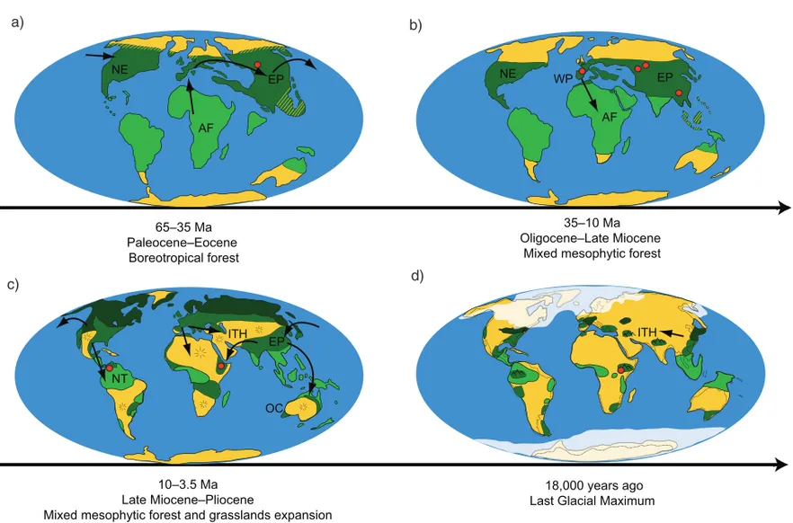
Fifty-ﬁve million years ago, the Earth experienced one of the warmest intervals in history, with global temperatures up to 10°warmer than present and tropical

climates characterizing northern latitudes (Zachos et al.

2008). The boreotropical ﬂora, a mixture of hardwood

deciduous and evergreen tropical taxa with no analog today, extended across North America and Eurasia

(Fig. 6a, Tiffney 1985, Wolfe 1975). The ancestors of

family Hypericaceae probably migrated from Africa to the Palearctic region during this warm Paleogene period and might have formed part of this boreotropical

ﬂora about 50 million years ago (Node 142, Fig. 4).

Our bioclimate model for the Early Eocene, however, does not support this scenario, showing that the tropical regions of the Southern Hemisphere and a large area in the Holarctic where, the boreotropical forest

was distributed (Fig. 6a), as climatically unfavorable

(Fig. 2a). Nevertheless, the fossil record of Hypericum

only extends back to 35 Ma, and the Early Eocene bioclimatic model is only based on Late Eocene to Mid-Miocene occurrences. Thus, it is possible that this ENM reconstruction does not correctly represents the potential