Co-variations between plant functional traits emerge from constraining parameterization of a terrestrial biosphere model

HAL Id: hal-02371849

https://hal.archives-ouvertes.fr/hal-02371849

HAL is a multi-disciplinary open access archive for the deposit and dissemination of sci-entific research documents, whether they are pub-lished or not. The documents may come from teaching and research institutions in France or abroad, or from public or private research centers.

L’archive ouverte pluridisciplinaire HAL, est destinée au dépôt et à la diffusion de documents scientifiques de niveau recherche, publiés ou non, émanant des établissements d’enseignement et de recherche français ou étrangers, des laboratoires publics ou privés.

Co-variations between plant functional traits emerge

from constraining parameterization of a terrestrial

biosphere model

Marc Peaucelle, Cédric Bacour, Philippe Ciais, Nicolas Vuichard, Sylvain

Kuppel, Josep Peñuelas, Luca Belelli Marchesini, Peter Blanken, Nina

Buchmann, Jiquan Chen, et al.

To cite this version:

Marc Peaucelle, Cédric Bacour, Philippe Ciais, Nicolas Vuichard, Sylvain Kuppel, et al.. Co-variations between plant functional traits emerge from constraining parameterization of a terrestrial biosphere model. Global Ecology and Biogeography, Wiley, 2019, 27 (9), pp.1351-1365. �10.1111/geb.12937�. �hal-02371849�

Co-variations between plant functional traits emerge from constraining 1

parameterization of a terrestrial biosphere model. 2

Running title: Functional traits variability inferred from data assimilation 3

4

Marc Peaucelle1,2, Cédric Bacour3, Philippe Ciais1, Nicolas Vuichard1, Sylvain Kuppel4, 5

Josep Peñuelas2,5, Luca Belelli Marchesini6,7, Peter D. Blanken8, Nina Buchmann9, Jiquan 6

Chen10, Nicolas Delpierre11, Ankur Desai12, Eric Dufrene11, Damiano Gianelle6, Cristina 7

Gimeno-Colera13, Carsten Gruening14, Carole Helfter15, Lukas Hörtnagl9, Andreas Ibrom16, 8

Richard Joffre17, Tomomichi Kato18,19, Thomas E. Kolb20, Beverly Law21, Anders Lindroth22, 9

Ivan Mammarella23, Lutz Merbold24, Stefano Minerbi25, Leonardo Montagnani25,26, Ladislav 10

Šigut27

, Mark Sutton15, Andrej Varlagin28, Timo Vesala29,30, Georg Wohlfahrt31, Sebastian 11

Wolf32, Dan Yakir33 and Nicolas Viovy1. 12

1Laboratoire des Sciences du Climat et de l'Environnement, CEA/CNRS/UVSQ, Gif-sur-Yvette, France 13

2CREAF, Cerdanyola del Vallès, Barcelona 08193, Catalonia, Spain 14

3NOVELTIS, Labège, France 15

4Northern Rivers Institute, School of Geosciences, University of Aberdeen 16

5CSIC, Global Ecology Unit CREAF -CSIC-UAB, Bellaterra, Barcelona 11 08193, Catalonia, Spain 17

6Department of Sustainable Agro-Ecosystems and Bioresources, Research and Innovation Centre, Fondazione 18

Edmund Mach, San Michele all'Adige, Italy 19

7Department of Landscape Design and Sustainable Ecosystems, Agrarian-Technological Institute, RUDN 20

University, Moscow, Russia 21

8Department of Geography, University of Colorado, Boulder, Colorado 22

9Institute of Agricultural Sciences, ETH Zurich, Zurich, Switzerland 23

10LEES Lab, Department of Geography and Spatial Sciences, Michigan State University, East Lansing, 24

Michigan 25

11Ecologie Systématique Evolution, Univ. Paris-Sud, CNRS, AgroParisTech, Université Paris-Saclay, Orsay, 26

France 27

12Department of Atmospheric and Oceanic Sciences, University of Wisconsin–Madison, Madison, Wisconsin 28

13Fundación CEAM, Parque Tecnológico, Paterna, Spain 29

14European Commission, Joint Research Centre, Ispra, Italy 30

15Centre for Ecology and Hydrology, Penicuik, UK 31

16Department of Environmental Engineering, Technical University of Denmark, Lyngby, Denmark 32

17CEFE, CNRS – Université de Montpellier – Université Paul-Valéry Montpellier – EPHE – IRD, Montpellier, 33

France 34

18Research Faculty of Agriculture, Hokkaido University, Sapporo, Japan 35

19Global Station for Food, Land and Water Resources (GSF), GI-CoRE, Hokkaido University, Sapporo, Japan 36

20School of Forestry, Northern Arizona University, Flagstaff, Arizona 37

21Forest Ecosystems and Society Dept, College of Forestry, Oregon State University, Corvallis, Oregon 38

22Department of Physical Geography and Ecosystem Science, Lund University, Lund, Sweden 39

23Institute for Atmosphere and Earth System Research/Physics, Faculty of Science, University of Helsinki, 40

Helsinki, Finland 41

24Mazingira Centre, International Livestock Research Institute (ILRI), Nairobi, Kenya 42

25Forest Services, Autonomous Province of Bolzano, Bolzano, Italy 43

26Faculty of Science and Technology, Free University of Bolzano, Piazza Università, Bolzano, Italy 44

27Department of Matter and Energy Fluxes, Global Change Research Institute CAS, Brno, Czech Republic 45

28A.N. Severtsov Institute of Ecology and Evolution, Russian Academy of Sciences, Moscow, Russia 46

29Institute for Atmosphere and Earth System Research/Forest Sciences, Faculty of Agriculture and Forestry, 47

University of Helsinki, Helsinki, Finland 48

30Viikki Plant Science, University of Helsinki, Helsinki, Finland 49

31Institute for Ecology, University of Innsbruck, Innsbruck, Austria 50

32Institute of Terrestrial Ecosystems, ETH Zurich, Zurich, Switzerland 51

33Earth and Planetary Sciences, Weizmann Institute of Science, Rehovot, Israel 52

53

Marc Peaucelle: [email protected] (corresponding author) 54

55

Acknowledgments 56

This work was performed using HPC resources from GENCI-TGCC (Grant

2017-57

A0030106328). The authors would like to acknowledge the financial support from the

58

European Research Council Synergy grant ERC-SyG-2013-610028 IMBALANCE-P. The

59

study was supported by the National Centre of Excellence (272041), ICOS-Finland (281255)

60

and Academy professor project (284701) funded by the Academy of Finland. N.B.

61

acknowledges various funding sources for the Swiss FluxNet, particularly from the SNF

62

(grants: 20FI21_148992, 20FI20_173691). L.M. was supported by the Swiss National Science

63

Foundation under the 40FA40_154245/1 grant agreement. This work used eddy covariance

64

data acquired and shared by the FLUXNET community, including these networks:

65

AmeriFlux, AfriFlux, AsiaFlux, CarboAfrica, CarboEuropeIP, CarboItaly, CarboMont,

66

ChinaFlux, Fluxnet-Canada, GreenGrass, ICOS, KoFlux, LBA, NECC, OzFlux-TERN,

67

TCOS-Siberia, and USCCC. The ERA-Interim reanalysis data are provided by ECMWF and

68

processed by LSCE. The FLUXNET eddy covariance data processing and harmonization was

69

carried out by the European Fluxes Database Cluster, AmeriFlux Management Project, and

70

Fluxdata project of FLUXNET, with the support of CDIAC and ICOS Ecosystem Thematic

71

Center, and the OzFlux, ChinaFlux and AsiaFlux offices. L.B.M. acknowledges the support of 72

the RUDN University program 5‐100. L L.Š. was supported by the Ministry of Education, 73

Youth and Sports of CR within the National Sustainability Program I (NPU I), grant number 74 LO1415. 75 76 77 78

Co-variations between plant functional traits emerge from constraining 79

parameterization of a terrestrial biosphere model. 80

Running title: Functional traits variability inferred from data assimilation 81

Key words: Plant functional traits, ORCHIDEE, terrestrial model, optimization, data 82

assimilation, plant acclimation. 83 84 Abstract 85 Aim 86

Mechanisms of plant trait adaptation and acclimation are still poorly understood and 87

consequently lack a consistent representation in terrestrial biosphere models (TBMs). Despite 88

the increasing availability of geo-referenced trait observations, current databases are still 89

insufficient to cover all vegetation types and environmental conditions. In parallel, the 90

growing number of continuous eddy-covariance observations of energy and CO2 fluxes has 91

enabled modelers to optimize TBMs with these data. Past attempts to optimize TBMs 92

parameters mostly focused on model performance overlooking the ecological properties of 93

ecosystems. The aim of this study is to assess the ecological consistency of optimized trait-94

related parameters while improving the model performances for gross primary productivity 95 (GPP) at sites. 96 Location 97 World 98 Time period 99 1992-2012 100

Major taxa studied 101

Trees and C3 grasses 102

Methods 103

We optimized parameters of the ORCHIDEE model against 371 site-years of GPP estimates 104

from the FLUXNET network and we looked at global co-variation among parameters and 105

with climate. 106

Results 107

The optimized parameter values are shown to be consistent with leaf-scale traits, in particular 108

well-known trade-offs observed at the leaf level, echoing the leaf economic spectrum theory. 109

Results show a marked sensitivity of trait-related parameters to local bio-climatic variables 110

and reproduce observed relationships between traits and climate. 111

Main conclusions 112

Our approach validates some biological processes implemented in the model and enables us 113

to study ecological properties of vegetation at the canopy level, as well as some traits that are 114

difficult to observe experimentally. This study stresses the need for 1) implementing explicit 115

trade-offs and acclimation processes in TBMs, 2) improving the representation of processes to 116

avoid model-specific parameterization as well as 3) performing systematic traits 117

measurements at FLUXNET sites in order to gather information on plant ecophysiology and 118

plant diversity, together with micro-meteorological conditions. 119

Introduction 121

Terrestrial biosphere models (TBMs) describe the different processes controlling exchanges 122

of energy and trace gases between the atmosphere and the biosphere. Process-based TBMs are 123

useful tools for understanding the dynamics of ecosystems under changing environment, for 124

present-day to future conditions. 125

In most TBMs, the worldwide vegetation is divided into plant functional types (PFTs) based 126

on general characteristics of the photosynthetic pathways, phenology, structure and 127

physiology. Different PFTs usually share the same equations but use different parameter 128

values to describe generic processes (photosynthesis, respiration), while biome-specific 129

equations may be used for phenology and allocation. Therefore, for a given PFT, only the 130

differences in climate and soil properties can determine spatial and temporal gradients in 131

ecosystem state variables. 132

The prescribed values of PFT-specific parameters are derived from discrete observations 133

obtained at varying spatial scales (organs, individuals, ecosystems; Reich et al., 2007; Kattge 134

et al., 2009) and in specific environmental conditions, despite the modulation of real world

135

plant traits by climate (Wright et al., 2005; Ordoñez et al., 2009; van Ommen Kloeke et al., 136

2012; Maire et al., 2015) and soil properties (Fisher et al., 2012). In addition, some TBM 137

parameters relate to traits that are difficult to measure experimentally (e.g. root turnovers or 138

carbon allocation), or are model-specific. These parameters can hardly be directly optimized 139

from observations and their adjustment to varying environmental conditions can only be 140

determined by labor intensive multi-factorial ecosystem manipulation experiments (Luo et al., 141

2017). This rigid determination of parameter values, combined with the use of single PFT to 142

cover a range of different species (Peaucelle et al., 2016), hinders a realistic representation of 143

the past, present and future ecosystem dynamics both at the local or regional scale, and their 144

response to global drivers such as climate, elevated CO2 and nutrient fertilization (Hartig et 145

al., 2012, Atkin et al., 2015; Kroner & Way, 2016; Reich et al., 2016).

146

To overcome the rigidity of the PFT representation, various approaches have been proposed 147

to provide continuous distributions of plant functional traits related to model parameters. 148

These approaches range from extrapolating trait observations across spatial gradients 149

(Verheijen et al., 2015), to estimating optimal trait values according to ecological theories and 150

plant-centered approaches (Reu et al., 2011; Pavlick et al., 2013; Prentice et al., 2014). The 151

drawback of these different approaches is that they require both spatial and temporal 152

observations for model calibration and/or validation. Despite the increasing number of geo-153

referenced trait observations (Kattge et al., 2011), current databases are insufficient to cover 154

all vegetation types and environmental conditions for projections at the ecosystem level 155

(Musavi et al., 2015, 2016). Moreover, trait observations should be co-located with process 156

and meteorology data to understand linkages between traits and ecosystem function (Law et 157

al., 2008), which is rare in existing databases although increasingly addressed for some

158

biomes (Bjorkman et al., 2018). Long-term monitoring of functional traits is needed to assess 159

the adjustments to climate. As such information is still lacking, approaches have been 160

developed that confound the spatial and temporal dimensions of trait variability. 161

Another modeling strategy consists in optimizing TBMs against observed variables sensitive 162

to ecosystem-level parameters in order to overcome these limitations. This approach assumes 163

that the model structure is unbiased, so that realistic parameters values can be estimated when 164

model simulations best match observations. Because biometric variables are sparse and often 165

depend on processes not represented in models (Thum et al., 2017), energy and trace gas flux 166

measurements are more appealing to optimize TBM parameters. Eddy-covariance data 167

provide near-continuous observations of CO2, latent heat and sensible heat fluxes, and are 168

therefore well suited for better constraining photosynthesis, respiration, transpiration and 169

carbon phenology model parameters. Eddy-covariance measurements have been extensively 170

used to improve specific performances of TBMs, i.e. their ability to reproduce specific 171

observed ecosystem behaviors (Carvalhais et al., 2010; Kuppel et al., 2012; Santaren et al., 172

2014; Schürmann et al., 2016). However, such model calibrations are disconnected, by 173

construction, from ecological theory or trait-based relationships, and do not exploit the full 174

potential of continuous flux observations across the globe, which provide both spatial and 175

temporal information. 176

In this study, we aim at assessing the consistency of model trait parameters optimized against 177

eddy-covariance flux tower measurements of growth primary productivity (GPP) using the 178

state-of-the-art ORCHIDEE land surface model (Krinner et al., 2005). In addition to classical 179

optimization analyses (i.e. looking for the optimal parameter sets resulting in the highest 180

model improvement), we focus here on the variability of optimized parameter values and on 181

inter-traits correlations or trait-environment correlations. By doing so, we address the 182

following research questions: 1) Are the parameters retrieved by optimizing the model against 183

flux tower records consistent with known relationships between traits (i.e. trade-offs) ? or 2) 184

between traits and environmental variables? and 3) What new relationship can be identified 185

with this approach? 186

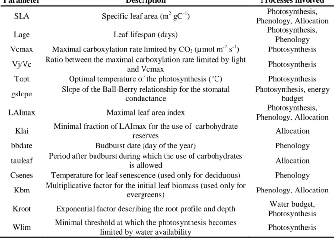
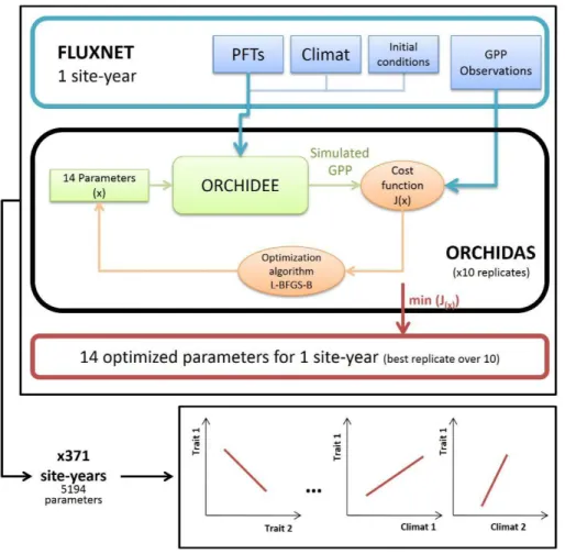
Methods 188

The ORCHIDEE model

189

The land surface model ORCHIDEE (v1.9.6, without nitrogen cycle) computes biosphere-190

atmosphere exchanges, consistently with water and carbon storage using ordinary differential 191

equations (Krinner et al., 2005) (Figure1). Given meteorological forcing, plant and soil 192

conditions, the model simulates photosynthesis, all components of the surface energy budget 193

and hydrological processes at a half-hourly time step, while the dynamics of carbon storage 194

are calculated daily. In ORCHIDEE, the land surface is discretized into 12 plant functional 195

types (PFT) and bare soil (Table S1.1, Appendix S1). All PFTs share the same equations, but 196

use different parameter values, except for phenology (budburst/senescence), which is PFT-197

specific (Botta et al., 2000). 198

199

Eddy-covariance GPP

200

We used half-hourly flux observations from eddy-covariance sites within the FLUXNET 201

network (https://fluxnet.fluxdata.org). The sites were selected on the basis of spatial 202

homogeneity and the dominance of a vegetation type that could easily be matched to one of 203

the PFTs in ORCHIDEE, excluding crops and C4 grasses. The vegetation type information at 204

each site was obtained from http://fluxnet.ornl.gov. The list of analyzed FLUXNET sites (98 205

sites, 371 site-year) and the corresponding PFTs is given in Appendix S2. The following 206

analyses rely on GPP derived from net ecosystem exchange (NEE; reference with variable 207

USTAR threshold) after accounting for ecosystem respiration calculated using the method of 208

Reichstein et al., (2005) provided in the FLUXNET dataset. Years with less than 80% of 209

available half hourly observations were discarded. 210

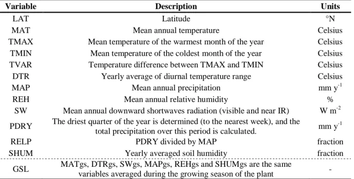
Meteorological data

212

Because ORCHIDEE needs continuous half-hourly meteorological forcing, we gap-filled time 213

series of weather variables using the interpolation algorithm developed by Vuichard & Papale 214

(2015). Linear interpolation was applied between available observations when the gap-215

duration in the meteorological data was less than six hours. Otherwise, the variables were 216

interpolated and bias corrected using the ERA-interim reanalysis (~80km, Dee et al., 2011). 217

Snow and rain were identified according to air temperature (threshold for snow being 0°C). 218

219

Data assimilation procedure

220

The parameters of ORCHIDEE were optimized with the ORCHIDAS package developed by: 221

Kuppel et al., (2012); Bacour et al., (2015); MacBean et al., (2015) and Peylin et al., (2016); 222

(https://orchidas.lsce.ipsl.fr/; Figure 1). Gaussian distributions of parameter and observation 223

errors being assumed, a gradient-based approach was used to minimize the Bayesian cost 224

function J (Tarantola, 2005): 225

_{( 1 )} This function quantifies the difference between observations (y) and simulations (H(x)) (here 226

GPP), and between a priori (xb) and optimized parameters (x). The B and R matrices are the 227

prior error covariance matrices for parameters and observations, respectively (including in the 228

latter case eddy-covariance measurement and model errors). 229

Both R and B were taken as diagonal, as discussed in Kuppel et al. (2012). The J(x) function 230

was iteratively minimized with the L-BFGS-B algorithm (Byrd et al., 1995), which notably 231

allows bounding the range of variation of the parameters to optimize. After model calibration 232

(i.e. minimizing J), the posterior error covariance matrix (A), providing the full statistical 233

distribution of the optimized parameters was estimated by: 234

_{( 2 )} where H is the Jacobian of model at the minimum of J (Tarantola, 2005). The covariances of 235

errors between parameters contained in the non-diagonal terms of A inform about the ability 236

of observations given the structure of H to solve for parameters individually, or in 237

combination. High error covariance between two parameters relates to the equifinality 238

problem, whereby different values of these parameters result in model outputs equally 239

matching the observations (relative to R). 240

241

Optimized parameters

242

We restricted our exercise to the parameters involved in the assimilation of CO2 following 243

previous sensitivity analyses from Kuppel (2012). We analyzed 14 parameters controlling 244

long-term and inter-annual GPP variability (Table 1). The key equations involving each 245

optimized parameter as well as their effect on the simulated GPP are described in Table S1.2 246

(Appendix S1). The parameters were related to photosynthetic capacity, phenology, carbon 247

allocation and the water budget. Photosynthetic capacity parameters were the maximal rate of 248

carboxylation limited by CO2 (Vcmax), the ratio between the maximal rate of carboxylation 249

limited by light and Vcmax (Vj/Vc), the optimal temperature of photosynthesis (Topt) and the 250

slope of the Ball-Berry model for stomatal conductance (gslope). Parameters driving 251

phenology were the specific leaf area (SLA), leaf longevity (Lage), summer maximal leaf area 252

index (LAImax) and the temperature for leaf senescence (Csenes). Allocation parameters were 253

the minimal fraction of LAImax for the use of carbohydrate reserves (Klai) and the period 254

after budburst during which the use of carbohydrates is allowed (tauleaf) for the formation of 255

new leaves. Finally, two parameters involved in the water status of the plant were the 256

exponential factor describing the root profile and length (Kroot) and the minimal threshold at 257

which photosynthesis becomes limited by minimum water potential (Wlim). In addition, two 258

scaling factor Kbm (initial biomass of leaves for evergreen species) and bbdate (spring 259

burdburst date) were added in the optimization to allow adjusting the seasonal timing of GPP. 260

The range in variation of the three parameters corresponding to observable traits (SLA, Vcmax 261

and Lage) was set from the TRY database for each PFT (Niinemets et al., 1999; Deng et al., 262

2004; Meir et al., 2007; Kattge et al., 2009, 2011; Domingues et al., 2010; Cernusak et al., 263

2011; Azevedo & Marenco, 2012; van de Weg et al., 2012; Nascimento & Marenco, 2013). 264

Species from the TRY database were assigned to corresponding PFTs based on available 265

metadata about plant structure, leaf phenology and climate information extracted from 266

species' latitude and longitude coordinates. We chose as a reference range the 2.5 - 97.5 267

percentile of the trait distributions from TRY. The variation ranges for the other parameters 268

were fixed based on expert judgment (Kuppel et al., 2014). 269

270

Simulations and assimilation set-up

271

At each flux tower site, we assumed that the eddy-covariance flux footprint was entirely 272

composed by a single PFT (Appendix S2). The model was forced by local meteorological 273

observations (see Meteorological data section) and soil texture from the harmonized 274

worldwide soil database (Nachtergaele et al., 2012) to define the residual and saturation water 275

contents, and the saturated hydraulic conductivity in the soil model (Ducoudré et al., 1993; 276

Krinner et al., 2005) based on Van Genuchten (1980). Initial soil carbon pools in equilibrium 277

with local climate were obtained with an analytical spin-up procedure (Lardy et al., 2011; Xia 278

et al., 2012). Initial biomass was simulated until reaching equilibrium (generally after a ~300

279

year-long simulations using the studied year meteorological data and constant CO2 set to level 280

of the year), thus different from the real stand age observed at each site. 281

We optimized GPP averaged over 15 days using moving windows to avoid noise from high 283

frequency variations in the parameter optimization that could induce convergence issues 284

(Bacour et al., 2015). As far as test data from eddy-covariance measurements are concerned, 285

high frequency variations in fluxes include also variation in the boundary layer that are 286

unrelated to the fluxes at the surface (Ibrom et al., 2006). Santaren et al. (2007) estimated that 287

for parameters related to photosynthesis and phenology, optimization based on half-hourly 288

observations did not improve the results. For each site, the optimizations were conducted 289

year-by-year to account for trait variability over time (Wu et al., 2013). 290

Following MacBean et al. (2015), each calibration (site-year) used ten replicates representing 291

different starting parameter sets with values randomly picked within their allowed variation 292

range (Table S1.3). Only the best calibration out of these ten replicates was retained for 293

analyses. This procedure increases the chances of finding the global minimum of J as 294

Santaren et al. (2014) showed that the gradient-based algorithm was sensitive to initial 295

conditions with a non-linear and complex model such as ORCHIDEE. 296

297

Analyses

298

We only retained calibrations for which the optimized model reproduced GPP observations 299

with high precision. The rationale for this was that optimized parameters from model runs 300

which agreed poorly with GPP observations provided little or no useable information. The 301

filtering was performed using a two-step procedure. 302

First, the criterion for ‘improved GPP simulation’ was the relative site-year posterior RMSE 303

(RMSEre) between observed and optimized GPP: 304

Whenever the value of RMSEre was higher than the all-RMSEre median plus one interquartile 305

range (IQR), the site-year was removed from the analysis. We also discarded sites with 306

‘inconsistent parameters values’, i.e. with too large differences between the ten replicates at 307

the same site reflecting convergence issues (equifinality) of the algorithm. 308

Secondly, for sites with at least two RMSEre below 10 % among the ten replicates, we 309

estimated the coefficient of variation (CV) of parameters across the replicates. We retained 310

only years for which the median CV was below the median of all CV plus one IQR of their 311

distribution. This filtering provided optimized parameters from 371 site-years (over 516 312

initially considered) for 98 sites (over 116; Appendix S2) spanning seven PFTs located in 313

boreal, temperate and tropical areas (Table S3.4; Appendix S3). 314

315

For each parameter, we calculated the uncertainty reduction (UR) as: 316

( 5 )

With post and prior being the posterior and prior parameter uncertainties (square root of the

317

diagonal elements of A and B). We then separated in the analysis the well- from the poorly-318

constrained parameters. Well-constrained parameters are defined as those with 1) UR higher 319

than the median of UR distributions for all parameters and 2) a low correlation of error with 320

other parameters (from the A matrix, Eq. 2). Note that a strong error correlation making two 321

parameters poorly constrained individually is still an interesting result as it indicates a range 322

of possible tradeoffs between these two parameters. 323

The optimized parameter values were regressed against the local background bio-climatic 324

variables (Table 2) for each site, and against the soil relative water content (volume of water 325

by volume of soil) simulated by ORCHIDEE. Bio-climatic variables were averaged over the 326

whole year and over the length of the growing season (GSL). For temperate sites, the growing 327

season was defined as the period with daily temperature above 5°C and relative soil water 328

content above 0.2 (Violle et al., 2015). In some tropical regions, the growing season length is 329

potentially limited by water availability (wet/dry seasons), we thus kept the same definition as 330

for temperate ecosystems. For boreal sites, we adapted the definition of the growing season 331

such as weekly temperature must be above 0°C. Analyses were performed with the R.3.2 332

software (R Core Team, 2016) and standardized major axis (SMA) analyses were performed 333

with the 'lmodel2' package (Legendre, 2014). Because we sought to compare simulated 334

correlations with common ecological properties observed at the global scale, we analyzed 335

different groups of PFTs: all PFTs together; deciduous versus evergreens; needleleaves versus 336

broadleaves; and C3 grasses (Table S1.1). Regressions were performed both with and without 337

a logarithmic transformation of the data. 338

Results and comparison to existing literature 339

Optimization performances

340

A full description of the optimization performances and parameter uncertainty reduction can 341

be found in Appendix S3. 342

In all cases, the optimized GPP time series better agrees with observations than the prior ones, 343

with the RMSE being reduced by 76.6 ± 13.0 % (Table S3.4; Appendix S3). The median 344

posterior RMSEre is 0.19 and the IQR is 0.11. The median CV over all parameters is 0.24 345

(IQR=0.13). After optimization, the parameter uncertainty (Eq. 5) is reduced by 30 % on 346

average (Table S3.5; Appendix S3). 347

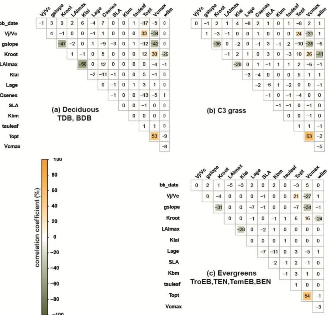
The posterior error correlation matrix A (Eq.2) reveals a positive correlation between Vcmax 348

and several other parameters including (Figure 2): Topt (r=0.57±0.05); gslope (r=-0.37±0.04); 349

Kroot (r=0.24±0.07) and Vj/Vc (r=-0.31±0.04). There also exists a negative correlation

350

between Kroot and gslope (r=-0.38±0.08), between Kroot and Wlim (r=-0.30±0.09) and 351

between LAImax and Klai (r=-0.37±0.16) (Figure 2). 352

Jointly analyzing information from the uncertainty reduction (Appendix S3) and the cross-353

parameter error correlation enables to distinguish between: 1) well constrained parameters 354

(Lage and SLA for evergreens/ Lage and Csenes for deciduous); 2) well constrained 355

parameters with a risk of equifinality (gslope, Kroot, LAImax, Topt and Vcmax); and 3) poorly 356

constrained parameters (Vj/Vc, Klai, Tauleaf and Wlim; Table 1). In the following analyses, 357

trait co-variations have to be interpreted in respect to confidence intervals (posterior error) in 358

parameter estimates. 359

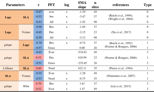
Co-variation between parameters

360

We analyzed cross-site correlations between optimized parameters in relation to expected trait 361

relationships. The co-variation between all parameters is illustrated in Figure S4.2 (Appendix 362

S4). For more clarity and considering the large number of parameters, we only describe here 363

the relationships involving four parameters related to phenology (SLA, Lage) and 364

photosynthesis (Vcmax, gslope). All relationships are provided in Table S4.6 (Appendix S4). 365

We observed a negative correlation between SLA and Lage for all PFTs (r=-0.63; Table 3) as 366

well as for evergreens (r=-0.67) and broadleaves PFTs (r=-0.53), separately. The slope of the 367

emerging relationship between LMA (1/SLA) and Lage (1.91; 1.63-2.24 95% confidence 368

interval; p < 0.05) for all PFTs was close to the observed slope from field observations (1.71; 369

1.62-1.82; Wright et al. 2004). Results highlighted other co-variations between Lage and 370

Vcmax (r=-0.59 overall PFTs), gslope and Lage (r=-0.7 for broadleaves), LAImax and SLA

371

(r=0.6 for needleleaves), and between SLA and Vcmax (r=-0.55 for evergreens). Here again, 372

the slope between Lage and Vcmax emerging for broadleaves PFTs (-1.69) was close to 373

observations (-1.13; Xu et al. 2017). 374

No relationships were reported between gslope and Lage or between glsope and SLA, but a 375

trade-off between the stomatal conductance (gs) and Lage was observed experimentally 376

(Reich et al., 1992; Poorter & Bongers, 2006), as well as a positive correlation between gs 377

and SLA (Poorter & Bongers, 2006). The optimizations showed opposite relationships 378

between gslope and SLA depending on the PFT: a positive significant correlation was 379

obtained for deciduous PFTs and a negative significant correlation for evergreens and grasses 380

(Table 3). 381

The positive relationship between SLA and LAImax emerging from optimized parameters for 382

coniferous PFTs was consistent with the positive correlation between LAI and SLA reported 383

by Pierce et al. (1994) for coniferous forests. Finally, a negative correlation between SLA and 384

Vcmax has been observed experimentally for two gymnosperms species (Niinemets et al.,

385

2007), confirming the negative relationships found in our study for needleleaves. Despite the 386

equifinality risk between gslope and the soil water stress Wlim in Figure 2, the positive 387

correlation observed for broadleaves (r=0.7) and evergreens (r=0.52) was comparable to 388

observations from independent data compiled by Lin et al. (2015). 389

Other significant correlations from the optimized parameters (Table S4.6, Figure S4.2; 390

Appendix S4) could not be verified against observations because of the correlation of errors 391

observed in Figure 2 or because of the scarcity of ecological data preventing us to conclude 392

about the true nature of those correlations, as for example between gslope and Vcmax. 393

394

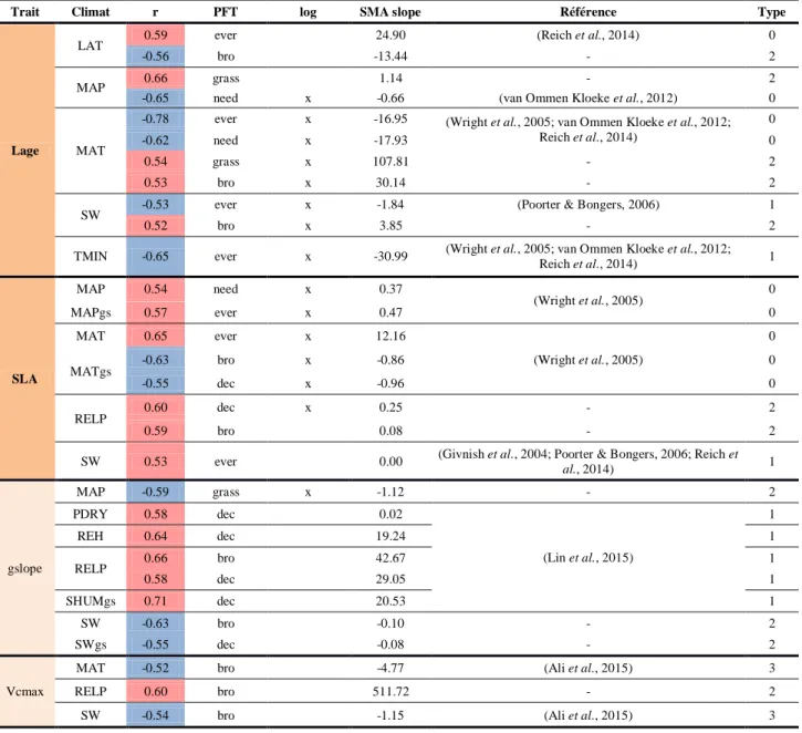
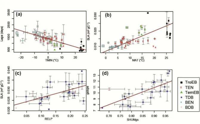
Variation of trait-related parameters with climate

395

We analyzed correlations between parameters and climate variables (Table 4, Figure S5.4; 396

Appendix S5). As for co-variations between parameters, we only described here those 397

implying SLA, Lage, Vcmax and gslope. All relationships are listed in Table S5.7 and more 398

detailed analysis are available in Appendix S5. 399

We found a strong negative correlation between leaf lifespan (Lage) and temperatures (MAT, 400

TMIN; r=-0.78/-0.65; Figure 3a) for evergreen PFTs. This correlation was independently

401

reported at global scale (Wright et al., 2005; van Ommen Kloeke et al., 2012) and confirmed 402

by Reich et al. (2014) who showed higher needle longevity with cold temperatures for boreal 403

species. However, the observed positive correlation between Lage and MAT at the global 404

scale for deciduous PFTs (Wright et al., 2005; van Ommen Kloeke et al., 2012) was not 405

found specifically for deciduous systems in our study. Nevertheless, a positive correlation was 406

observed for C3 grasses and broadleaves (including deciduous). We also found a strong 407

negative correlation between Lage and the mean annual precipitations (MAP) for evergreens 408

PFTs (r = -0.65), consistent with field data (van Ommen Kloeke et al., 2012). In addition, a 409

negative correlation between Lage and incident shortwave radiation (SW) for evergreens was 410

obtained, consistent with field observations (Poorter & Bongers, 2006). 411

412

Regarding SLA, we found opposite sensitivities to MAT for evergreen (r=0.65) and deciduous 413

forests (r=-0.55). This result is consistent with independent leaf-scale data showing a positive 414

correlation between SLA and MAT for evergreen species (Figure 3b) and a negative 415

correlation for deciduous ones (Wright et al. 2005). The model calibration also resulted in a 416

positive correlation between the relative precipitation (RELP; Table 2) and SLA for deciduous 417

trees (r = 0.60; Figure 3c). Regarding the positive correlations obtained between SLA with 418

Kroot or gslope (Table 3), it suggests that SLA is highly sensitive to water stress for deciduous

419

trees. For evergreens, positive correlation between SLA and precipitation also emerges when 420

considering the length of the growing season (MAPgs, r = 0.57; Table 4); which is consistent 421

with trait data (Wright et al., 2005). For evergreens, SLA was positively correlated to SW 422

(r=0.53), a relationship observed by Givnish et al. (2004) and Poorter & Bongers (2006). 423

424

In their meta-analysis of stomatal conductance parameters from observations of several PFTs, 425

Lin et al. (2015) showed that the slope of the stomatal conductance is positively correlated to 426

the mean air temperature over the growing period and to soil moisture stress. Here, our results 427

show the same correlation between gslope and soil moisture during the growing season 428

(r=0.71; Figure 3d) and relative precipitation (r=0.66) for deciduous or broadleaved PFTs. On 429

the contrary, we find that gslope is negatively correlated with mean annual precipitation for 430

C3 grasses (r=-0.59), and with shortwave radiation for broadleaved PFTs (r=-0.63). Medlyn et 431

al. (2011) suggested that gslope is proportional to the photosynthesis compensation point for

432

CO2, and consequently to growth temperatures of the plant (Bernacchi et al., 2001). This 433

assumption is supported by the data from Lin et al. (2015). In our study, the relationship 434

between gslope and temperature was not supported. 435

436

Finally, Vcmax is mostly sensitive to temperature and light for broadleaved PFTs, with a 437

negative correlation observed with MAT (r=-0.52) and SW (r=-0.54). This result contradicts 438

previous observations by Ali et al. (2015), who suggested a positive correlation between 439

Vcmax and seasonal temperature and light variations.

440 441

Discussion 442

Uncertainties and shortcomings of the approach

443

This section provides an overview of possible shortcomings of our approach that may explain 444

some residual mismatch between model and observations. Several factors can impact the 445

optimized value of the parameters, potentially aliasing the observed relationships: 1) flux 446

measurements errors and errors in ecosystem respiration estimates used to derive gap-filled 447

GPP; 2) optimization protocol/setup errors; and 3) model systematic errors deriving from 448

absent or poorly represented processes in the model. 449

First, we restricted our analysis to GPP. This flux is not directly measured but estimated from 450

NEE measured using the eddy-covariance method with an estimate of ecosystem respiration 451

determined using empirical models (Reichstein et al., 2005), and thus can be biased by 452

several factors (see Appendix S3 for a list of these factors). We chose GPP over a 453

combination of NEE and latent heat or evapotranspiration fluxes, which has often been used 454

to optimize ORCHIDEE (Kuppel et al., 2012; Bacour et al., 2015; Peylin et al., 2016), 455

because it implies the optimization of more parameters related to soil, respiration and energy 456

budget, and therefore increases the risk of equifinality. To reduce the uncertainties, it is 457

necessary to lower the correlation of errors between parameters by assimilating 458

complementary biophysical variables. For example, assimilating both GPP and LAI estimates 459

at the site level could improve the evaluation of parameters such as SLA or Lage, and 460

consequently improve the estimation of photosynthesis parameters. 461

Second, the Bayesian framework is based on the assumption that the model/observation errors 462

are random and that the model structure is “true”. Any bias of model structure is expected to 463

be aliased onto the estimated parameters (MacBean et al., 2016) and might therefore impact 464

the retrieved correlations. For instance, missing processes would be compensated during the 465

optimization by adjusting parameters (e.g. light attenuation, vertical distribution of LAI, 466

diffuse light, horizontal light distribution in the stand) to non optimal values. Also, while 467

traits are usually measured at the leaf level, our approach rather focuses on traits at the canopy 468

level (given the structure of ORCHIDEE and the assumed exponential attenuation of light and 469

LAI from top to bottom of canopy (Krinner et al. 2005; Table S1.2), and the assimilation of 470

GPP data). As an additional test, we conducted the above analyses using multi-year instead of 471

single-year observations in order to add more constraints on parameters (see Figure S4.3 & 472

S5.5). The same relationships were found as with single-year observations, thus strengthening 473

our conclusions, showing that spatial correlations are observed even when taking into account 474

a possible temporal variability of traits. 475

Finally, a wrong representation of species and the lack of representation of representation of 476

traits variability within a community in ORCHIDEE can affect simulated processes, which 477

will ultimately impact the estimated parameter values (see Appendix S3 for a discussion on 478

initial site conditions). Especially, the C3 grass PFT represents diverse grasslands, with 479

different species, ecophysiology (Adams et al., 2016) and management practices (Merbold et 480

al., 2014). This results in an increased variability and a high range of estimated plant

481

functional traits (Figure S3.1). A refinement of the PFT definition may improve the 482

robustness of optimizations (for instance by separating natural or semi-managed biomes), or 483

by distinguishing genera or major species (Peaucelle et al., 2016). 484

In order to decrease the impact of uncertainty in PFT composition and reduce the correlation 485

errors between parameters, the use of concomitant observations of traits and carbon fluxes at 486

the FLUXNET sites would enable a) to constrain known parameters and b) to validate 487

optimized traits. However, functional trait observations at FLUXNET sites as well as a 488

precise description of species composition are not yet systematic (Musavi et al., 2015, 2016). 489

490

Ecological consistency of trait relationships

491

The optimization of model parameters managed to reproduce many known ecological 492

properties. The optimized parameters consistently matched the well-known relationships 493

resulting from the leaf economic spectrum theory (LES, Reich et al., 1999; Wright et al., 494

2004). Particularly our results align with the trait theory that long lived canopies are 495

metabolically less active and are consistent with the LES empirical evidence that plants invest 496

either in structure or photosynthesis (Liu et al., 2010; Reich, 2014). 497

Our results also reproduced several observed trait-climate relationships at the PFT level. 498

Globally, evergreen PFT parameters showed a strong dependency on mean annual 499

temperature and radiation, while parameters for deciduous PFTs exhibited a strong sensitivity 500

to precipitation and soil moisture over the growing season (Figure S5.4). As postulated by 501

Reich (2014), climate exerts a control on the average leaf characteristics at the community 502

level. The observed relationships obtained at the PFT level might reflect, not only differences 503

in plant response to climate, but also differences in plant community composition (Shi et al., 504

2015). These results suggest that both the development of acclimation processes and trait-505

based approaches are needed in TBMs if we seek to capture the effect of biogeography on 506

ecosystem characteristics (Lu et al., 2017; Fisher et al., 2018). 507

508

Finally, while the results clearly highlight that photosynthesis and phenological mechanisms 509

implemented in ORCHIDEE are robust enough to reproduce known behaviors of several 510

vegetation species, belowground processes still appear poorly represented, which resulted in 511

weakly constrained parameters and trait co-variations inconsistent with literature. These 512

discrepancies are primarily due to a lack in eco-physiological knowledge reflecting the actual 513

difficulty to study belowground ecological processes. The rooting system uses model-specific 514

parameters (Kroot) that are hardly comparable to measured functional traits. 515

516

Concluding remarks and recommendations 517

The approach presented in this study is a new and effective way to validate the processes 518

implemented in TBMs, to better define vegetation response to climate (Liang et al., others, 519

2018), and could help improving existing data assimilation frameworks (Kaminski et al., 520

2013; LeBauer et al., 2013; Arsenault et al., 2018) by bringing ecological constraints. The 521

availability of continuous observations from eddy-covariance flux measurements gives a 522

unique opportunity to resolve the different components of the short and long-term variability 523

of traits through this approach. 524

Our results show that optimized leaf-related parameters align with plant trait theory, and 525

highlight the need to implement acclimation processes and trait-based approaches in models 526

instead of using constant parameters to reduce uncertainties in spatio-temporal patterns of the 527

modeled carbon fluxes. A first step would be to assess the behavior of the model at the global 528

scale when trait-climate relationships characterized in this study are explicitly implemented. 529

In parallel, relationships highlighted in this study may help to develop or validate new 530

methods to simulate plant acclimation. Used in a prognostic way, this approach could enable 531

to study correlations at the canopy scale and to assess the behavior of trait-related parameters 532

that are difficult to observe experimentally. 533

Several known ecological properties, observed at the site/leaf scale, emerged from model-data 534

assimilation. However, quantitative comparisons with observations were possible only for two 535

of them, SLA and Lage, which are also the two most studied traits. This is mainly because 536

TBMs use model-specific parameters that cannot be directly compared to standard trait 537

observations, but also because concomitant observations of functional traits, both in space and 538

time, are scarce in the literature. A recommendation to the TBM community would be to 539

make use of parameters (and processes) that can be related directly to observations in order to 540

unit vegetation model and functional traits (for instance the use of the Specific Root Length 541

for belowground processes). 542

We argue that co-located systematic and standardized trait observations (starting with key 543

traits related to phenology SLA, LAI, photosynthesis Vcmax, Jmax, Topt, water transport -544

gs- and allocation -Carbon:Nitrogen ratio, shoot/root-; (Law et al., 2008) along with

545

biometric data are needed at the FLUXNET sites or within other environmental observation 546

networks such as ICOS (Integrated Carbon Observation System) or NEON (National 547

Ecological Observatory Network) if we seek to distinguish temporal and spatial components 548

of trait variability across biomes and climates. The creation of a FLUXNET trait database 549

could improve our comprehension of trait acclimation and help us to disentangle the 550

differences observed at regional and local scales, to improve the up-scaling of processes from 551

the leaf to the canopy/ecosystem level and to properly calibrate/validate ecosystem models. 552

Supporting information 553

Appendix S1: Description of PFTs, model parameters and equations 554

Table S1.1: List of plant functional types. 555

Table S1.2: List of main equations involving optimized parameters. 556

Table S1.3: Default parameter value and range allowed by the optimization algorithm. 557

Appendix S2: List of FLUXNET sites used for the analyses (xlsx file). 558

Appendix S3: Optimization performances 559

Figure S3.1: Distribution of optimized parameter values. 560

Table S3.4: Mean a priori and a posteriori RMSE between observations and simulations. 561

Table S3.5: Mean parameter uncertainty reduction between prior and posterior simulations. 562

Appendix S4: Relationships between traits 563

Figure S4.2: Correlation matrices between traits optimized against site-year GPP. 564

Figure S4.3: Correlation matrices between traits optimized against site GPP. 565

Table S4.6: Extended Table 3 with all relationships 566

Appendix S5: Relationships between traits and climate 567

Figure S5.4: Correlation matrices between traits and environmental variables optimized 568

against site-year GPP 569

Figure S5.5: Correlation matrices between traits and environmental variables optimized 570

against site GPP 571

Table S5.7: Extended Table 4 with all relationships 572

573

Data accessibility 574

All FluxNet data can be downloaded at: https://fluxnet.fluxdata.org 575

Information about the ORCHIDEE model, source code and contact: http://orchidee.ipsl.fr/ 576

Information about the data assimilation system ORCHIDAS: https://orchidas.lsce.ipsl.fr/ 577

578 579

References 580

Adams, M.A., Turnbull, T.L., Sprent, J.I. & Buchmann, N. (2016) Legumes are different: Leaf 581

nitrogen, photosynthesis, and water use efficiency. Proceedings of the National Academy of 582

Sciences, 113, 4098–4103.

583

Ali, A.A., Xu, C., Rogers, A., McDowell, N.G., Medlyn, B.E., Fisher, R.A., Wullschleger, S.D., 584

Reich, P.B., Vrugt, J.A., Bauerle, W.L. & others (2015) Global-scale environmental control of 585

plant photosynthetic capacity. Ecological Applications, 25, 2349–2365. 586

Arsenault, K.R., Kumar, S.V., Geiger, J.V., Wang, S., Kemp, E., Mocko, D.M., Beaudoing, H.K., 587

Getirana, A., Navari, M., Li, B. & others (2018) The Land surface Data Toolkit (LDT v7. 2)–a 588

data fusion environment for land data assimilation systems. Geoscientific Model Development, 589

11, 3605–3621. 590

Atkin, O.K., Bloomfield, K.J., Reich, P.B., Tjoelker, M.G., Asner, G.P., Bonal, D., Bönisch, G., 591

Bradford, M.G., Cernusak, L.A., Cosio, E.G., Creek, D., Crous, K.Y., Domingues, T.F., 592

Dukes, J.S., Egerton, J.J.G., Evans, J.R., Farquhar, G.D., Fyllas, N.M., Gauthier, P.P.G., 593

Gloor, E., Gimeno, T.E., Griffin, K.L., Guerrieri, R., Heskel, M.A., Huntingford, C., Ishida, 594

F.Y., Kattge, J., Lambers, H., Liddell, M.J., Lloyd, J., Lusk, C.H., Martin, R.E., Maksimov, 595

A.P., Maximov, T.C., Malhi, Y., Medlyn, B.E., Meir, P., Mercado, L.M., Mirotchnick, N., Ng, 596

D., Niinemets, Ü., O’Sullivan, O.S., Phillips, O.L., Poorter, L., Poot, P., Prentice, I.C., 597

Salinas, N., Rowland, L.M., Ryan, M.G., Sitch, S., Slot, M., Smith, N.G., Turnbull, M.H., 598

VanderWel, M.C., Valladares, F., Veneklaas, E.J., Weerasinghe, L.K., Wirth, C., Wright, I.J., 599

Wythers, K.R., Xiang, J., Xiang, S. & Zaragoza-Castells, J. (2015) Global variability in leaf 600

respiration in relation to climate, plant functional types and leaf traits. New Phytologist, 206, 601

614–636. 602

Azevedo, G. & Marenco, R. (2012) Growth and physiological changes in saplings of Minquartia 603

guianensis and Swietenia macrophylla during acclimation to full sunlight. Photosynthetica, 604

50, 86–94. 605

Bacour, C., Peylin, P., MacBean, N., Rayner, P., Delage, F., Chevallier, F., Weiss, M., Demarty, J., 606

Santaren, D., Baret, F. & others (2015) Joint assimilation of eddy covariance flux 607

measurements and FAPAR products over temperate forests within a process-oriented 608

biosphere model. Journal of Geophysical Research: Biogeosciences, 120, 1839–1857. 609

Bernacchi, C.J., Singsaas, E.L., Pimentel, C., Portis Jr, A.R. & Long, S.P. (2001) Improved 610

temperature response functions for models of Rubisco-limited photosynthesis. Plant, Cell & 611

Environment, 24, 253–259.

612

Bjorkman, A.D., Myers-Smith, I.H., Elmendorf, S.C., Normand, S., Thomas, H.J., Alatalo, J.M., 613

Alexander, H., Anadon-Rosell, A., Angers-Blondin, S., Bai, Y. & others (2018) Tundra Trait 614

Team: A database of plant traits spanning the tundra biome. Global Ecology and 615

Biogeography, 27, 1402–1411.

616

Botta, A., Viovy, N., Ciais, P., Friedlingstein, P. & Monfray, P. (2000) A global prognostic scheme of 617

leaf onset using satellite data. Global Change Biology, 6, 709–725. 618

Byrd, R.H., Lu, P., Nocedal, J. & Zhu, C. (1995) A limited memory algorithm for bound constrained 619

optimization. SIAM Journal on Scientific Computing, 16, 1190–1208. 620

Carvalhais, N., Reichstein, M., Ciais, P., Collatz, G.J., Mahecha, M.D., Montagnani, L., Papale, D., 621

Rambal, S. & Seixas, J. (2010) Identification of vegetation and soil carbon pools out of 622

equilibrium in a process model via eddy covariance and biometric constraints. Global Change 623

Biology, 16, 2813–2829.

624

Cernusak, L.A., Hutley, L.B., Beringer, J., Holtum, J.A. & Turner, B.L. (2011) Photosynthetic 625

physiology of eucalypts along a sub-continental rainfall gradient in northern Australia. 626

Agricultural and Forest Meteorology, 151, 1462–1470.

627

Dee, D., Uppala, S., Simmons, A., Berrisford, P., Poli, P., Kobayashi, S., Andrae, U., Balmaseda, M., 628

Balsamo, G., Bauer, P. & others (2011) The ERA-Interim reanalysis: Configuration and 629

performance of the data assimilation system. Quarterly Journal of the Royal Meteorological 630

Society, 137, 553–597.

Deng, X., Ye, W.-H., Feng, H.-L., Yang, Q.-H., Cao, H.-L., Xu, K.-Y. & Zhang, Y. (2004) Gas 632

exchange characteristics of the invasive species Mikania micrantha and its indigenous 633

congener M. cordata (Asteraceae) in South China. Botanical Bulletin of Academia Sinica, 45. 634

Domingues, T.F., Meir, P., Feldpausch, T.R., Saiz, G., Veenendaal, E.M., Schrodt, F., Bird, M., 635

Djagbletey, G., Hien, F., Compaore, H., Diallo, A., Grace, J. & Lloyd, J. (2010) Co-limitation 636

of photosynthetic capacity by nitrogen and phosphorus in West Africa woodlands. Plant, Cell 637

& Environment, 33, 959–980.

638

Ducoudré, N.I., Laval, K. & Perrier, A. (1993) SECHIBA, a new set of parameterizations of the 639

hydrologic exchanges at the land-atmosphere interface within the LMD atmospheric general 640

circulation model. Journal of Climate, 6, 248–273. 641

Fisher, J.B., Badgley, G. & Blyth, E. (2012) Global nutrient limitation in terrestrial vegetation. Global 642

Biogeochemical Cycles, 26, n/a–n/a.

643

Fisher, R.A., Koven, C.D., Anderegg, W.R., Christoffersen, B.O., Dietze, M.C., Farrior, C.E., Holm, 644

J.A., Hurtt, G.C., Knox, R.G., Lawrence, P.J. & others (2018) Vegetation demographics in 645

Earth System Models: A review of progress and priorities. Global change biology, 24, 35–54. 646

Van Genuchten, M.T. (1980) A closed-form equation for predicting the hydraulic conductivity of 647

unsaturated soils. Soil science society of America journal, 44, 892–898. 648

Givnish, T.J., Montgomery, R.A. & Goldstein, G. (2004) Adaptive radiation of photosynthetic 649

physiology in the Hawaiian lobeliads: light regimes, static light responses, and whole-plant 650

compensation points. American Journal of Botany, 91, 228–246. 651

Ibrom, A., Jarvis, P.G., Clement, R., Morgenstern, K., Oltchev, A., Medlyn, B.E., Wang, Y.P., 652

Wingate, L., Moncrieff, J.B. & Gravenhorst, G. (2006) A Comparative Analysis of Simulated 653

and Observed Photosynthetic CO2 Uptake in Two Coniferous Forest Canopies. Tree 654

Physiology, 26, 845–864.

655

Kaminski, T., Knorr, W., Schürmann, G., Scholze, M., Rayner, P., Zaehle, S., Blessing, S., Dorigo, 656

W., Gayler, V., Giering, R. & others (2013) The BETHY/JSBACH carbon cycle data 657

assimilation system: Experiences and challenges. Journal of Geophysical Research: 658

Biogeosciences, 118, 1414–1426.

659

Kattge, J., Díaz, S., Lavorel, S., Prentice, I.C., Leadley, P., Bönisch, G., Garnier, E., Westoby, M., 660

Reich, P.B., Wright, I.J., Cornelissen, J.H.C., Violle, C., Harrison, S.P., Van BODEGOM, 661

P.M., Reichstein, M., Enquist, B.J., Soudzilovskaia, N.A., Ackerly, D.D., Anand, M., Atkin, 662

O., Bahn, M., Baker, T.R., Baldocchi, D., Bekker, R., Blanco, C.C., Blonder, B., Bond, W.J., 663

Bradstock, R., Bunker, D.E., Casanoves, F., Cavender-Bares, J., Chambers, J.Q., Chapin Iii, 664

F.S., Chave, J., Coomes, D., Cornwell, W.K., Craine, J.M., Dobrin, B.H., Duarte, L., Durka, 665

W., Elser, J., Esser, G., Estiarte, M., Fagan, W.F., Fang, J., Fernández-Méndez, F., Fidelis, A., 666

Finegan, B., Flores, O., Ford, H., Frank, D., Freschet, G.T., Fyllas, N.M., Gallagher, R.V., 667

Green, W.A., Gutierrez, A.G., Hickler, T., Higgins, S.I., Hodgson, J.G., Jalili, A., Jansen, S., 668

Joly, C.A., Kerkhoff, A.J., Kirkup, D., Kitajima, K., Kleyer, M., Klotz, S., Knops, J.M.H., 669

Kramer, K., Kühn, I., Kurokawa, H., Laughlin, D., Lee, T.D., Leishman, M., Lens, F., Lenz, 670

T., Lewis, S.L., Lloyd, J., Llusià, J., Louault, F., Ma, S., Mahecha, M.D., Manning, P., 671

Massad, T., Medlyn, B.E., Messier, J., Moles, A.T., Müller, S.C., Nadrowski, K., Naeem, S., 672

Niinemets, Ü., Nöllert, S., Nüske, A., Ogaya, R., Oleksyn, J., Onipchenko, V.G., Onoda, Y., 673

Ordoñez, J., Overbeck, G., Ozinga, W.A., Patiño, S., Paula, S., Pausas, J.G., Peñuelas, J., 674

Phillips, O.L., Pillar, V., Poorter, H., Poorter, L., Poschlod, P., Prinzing, A., Proulx, R., 675

Rammig, A., Reinsch, S., Reu, B., Sack, L., Salgado-Negret, B., Sardans, J., Shiodera, S., 676

Shipley, B., Siefert, A., Sosinski, E., Soussana, J.-F., Swaine, E., Swenson, N., Thompson, K., 677

Thornton, P., Waldram, M., Weiher, E., White, M., White, S., Wright, S.J., Yguel, B., Zaehle, 678

S., Zanne, A.E. & Wirth, C. (2011) TRY – a global database of plant traits. Global Change 679

Biology, 17, 2905–2935.

680

Kattge, J., Knorr, W., Raddatz, T. & Wirth, C. (2009) Quantifying photosynthetic capacity and its 681

relationship to leaf nitrogen content for global-scale terrestrial biosphere models. Global 682

Change Biology, 15, 976–991.

683

Krinner, G., Viovy, N., Noblet-Ducoudré, N. de, Ogée, J., Polcher, J., Friedlingstein, P., Ciais, P., 684

Sitch, S. & Prentice, I.C. (2005) A dynamic global vegetation model for studies of the coupled 685

atmosphere-biosphere system. Global Biogeochemical Cycles, 19, 33 PP. 686

Kroner, Y. & Way, D.A. (2016) Carbon fluxes acclimate more strongly to elevated growth 687

temperatures than to elevated CO2 concentrations in a northern conifer. Global Change 688

Biology, 22, 2913–2928.

689

Kuppel, S. (2012) Assimilation de mesures de flux turbulents d’eau et de carbone dans un modèle de 690

la biosphère continentale, Versailles-St Quentin en Yvelines.

691

Kuppel, S., Peylin, P., Chevallier, F., Bacour, C., Maignan, F. & Richardson, A. (2012) Constraining a 692

global ecosystem model with multi-site eddy-covariance data. Biogeosciences, 9, 3757–3776. 693

Kuppel, S., Peylin, P., Maignan, F., Chevallier, F., Kiely, G., Montagnani, L. & Cescatti, A. (2014) 694

Model–data fusion across ecosystems: from multisite optimizations to global simulations. 695

Geoscientific Model Development, 7, 2581–2597.

696

Lardy, R., Bellocchi, G. & Soussana, J.-F. (2011) A new method to determine soil organic carbon 697

equilibrium. Environmental Modelling & Software, 26, 1759–1763. 698

Law, B.E., Arkebauer, T., Campbell, J.L., Chen, J., Sun, O., Schwartz, M., van Ingen, C. & Verma, S. 699

(2008) Terrestrial carbon observations: Protocols for vegetation sampling and data 700

submission. FAO, Rome. 701

LeBauer, D.S., Wang, D., Richter, K.T., Davidson, C.C. & Dietze, M.C. (2013) Facilitating feedbacks 702

between field measurements and ecosystem models. Ecological Monographs, 83, 133–154. 703

Legendre, P. (2014) lmodel2: Model II Regression. R package version 1.7-2, Available at: ht 704

tp://CRAN. R-project. org/package= lmodel2 (accessed 2 March 2015). 705

Liang, J., Xia, J., Shi, Z., Jiang, L., Ma, S., Lu, X., Mauritz, M., Natali, S.M., Pegoraro, E. & Penton, 706

C.R., others (2018) Biotic responses buffer warming-induced soil organic carbon loss in 707

Arctic tundra. Global change biology. 708

Lin, Y.-S., Medlyn, B.E., Duursma, R.A., Prentice, I.C., Wang, H., Baig, S., Eamus, D., de Dios, V.R., 709

Mitchell, P., Ellsworth, D.S. & others (2015) Optimal stomatal behaviour around the world. 710

Nature Climate Change, 5, 459–464.

711

Liu, G., Freschet, G.T., Pan, X., Cornelissen, J.H.C., Li, Y. & Dong, M. (2010) Coordinated variation 712

in leaf and root traits across multiple spatial scales in Chinese semi-arid and arid ecosystems. 713

New Phytologist, 188, 543–553.

714

Luo, Y., Jiang, L., Niu, S. & Zhou, X. (2017) Nonlinear responses of land ecosystems to variation in 715

precipitation. New Phytologist, 214, 5–7. 716

Lu, X., Wang, Y.-P., Wright, I.J., Reich, P.B., Shi, Z. & Dai, Y. (2017) Incorporation of plant traits in 717

a land surface model helps explain the global biogeographical distribution of major forest 718

functional types. Global Ecology and Biogeography, 26, 304–317. 719

MacBean, N., Maignan, F., Peylin, P., Bacour, C., Bréon, F.-M. & Ciais, P. (2015) Using satellite data 720

to improve the leaf phenology of a global terrestrial biosphere model. Biogeosciences, 12, 721

7185–7208. 722

MacBean, N., Peylin, P., Chevallier, F., Scholze, M. & Schürmann, G. (2016) Consistent assimilation 723

of multiple data streams in a carbon cycle data assimilation system. Geoscientific Model 724

Development, 9, 3569–3588.

725

Maire, V., Wright, I.J., Prentice, I.C., Batjes, N.H., Bhaskar, R., Bodegom, P.M., Cornwell, W.K., 726

Ellsworth, D., Niinemets, Ü., Ordonez, A. & others (2015) Global effects of soil and climate 727

on leaf photosynthetic traits and rates. Global Ecology and Biogeography, 24, 706–717. 728

Medlyn, B.E., Duursma, R.A., Eamus, D., Ellsworth, D.S., Prentice, I.C., Barton, C.V.M., Crous, 729

K.Y., De Angelis, P., Freeman, M. & Wingate, L. (2011) Reconciling the optimal and 730

empirical approaches to modelling stomatal conductance. Global Change Biology, 17, 2134– 731

2144. 732

Meir, P., Levy, P.E., Grace, J. & Jarvis, P.G. (2007) Photosynthetic parameters from two contrasting 733

woody vegetation types in West Africa. Plant Ecology, 192, 277–287. 734

Merbold, L., Eugster, W., Stieger, J., Zahniser, M., Nelson, D. & Buchmann, N. (2014) Greenhouse 735

gas budget (CO2, CH4 and N2O) of intensively managed grassland following restoration. 736

Global change biology, 20, 1913–1928.

737

Musavi, T., Mahecha, M.D., Migliavacca, M., Reichstein, M., van de Weg, M.J., van Bodegom, P.M., 738

Bahn, M., Wirth, C., Reich, P.B., Schrodt, F. & others (2015) The imprint of plants on 739

ecosystem functioning: A data-driven approach. International Journal of Applied Earth 740

Observation and Geoinformation, 43, 119–131.