3D Organ Property Mapping using Freehand
Ultrasound Scans
by
Alex Benjamin
S.M., Computation for Design and Optimization, Massachusetts
Institute of Technology (2017)
M.S., Mechanical Engineering, Drexel University (2015)
Submitted to the Department of Mechanical Engineering
in partial fulfillment of the requirements for the degree of
Doctor of Philosophy in Mechanical Engineering and Computational
Science and Engineering
at the
MASSACHUSETTS INSTITUTE OF TECHNOLOGY
September 2020
c
○ Massachusetts Institute of Technology 2020. All rights reserved.
Author . . . .
Department of Mechanical Engineering
August 25, 2020
Certified by . . . .
Brian W. Anthony
Principal Research Scientist
Thesis Supervisor
Accepted by . . . .
Nicolas Hadjiconstantinou
Chairman, Mechanical Engineering Committee on Graduate Students
3D Organ Property Mapping using Freehand Ultrasound
Scans
by
Alex Benjamin
Submitted to the Department of Mechanical Engineering on August 25, 2020, in partial fulfillment of the
requirements for the degree of
Doctor of Philosophy in Mechanical Engineering and Computational Science and Engineering
Abstract
3D organ property mapping has gained a considerable amount of interest in the re-cent years because of its diagnostic and clinical significance. Existing methods for 3D property mapping include computed tomography (CT), magnetic resonance imaging (MRI), and 3D ultrasound (3DUS). These methods, while capable of producing 3D maps, suffer from one or more of the following drawbacks: high cost, long scan times, computational complexity, use of ionizing radiation, lack of portability, and the need for bulky equipment. We propose the development of a framework that allows for the creation of 3D property maps at point of care (specifically structure and speed of sound). A fusion of multiple low-cost sensors in a Bayesian framework localizes a conventional 1D-ultrasound probe with respect to the room or the patient’s body; localizing the probe relative to the body is achieved by using the patient’s superfi-cial vasculature as a natural encoding system. Segmented 2D ultrasound images and quantitative 2D speed of sound maps obtained using numeric inversion are stitched together to create 3D property maps. A further advantage of this framework is that it provides clinicians with dynamic feedback during freehand scans; specifically, it dynamically updates the underlying structural or property map to reflect high and low uncertainty regions. This allows clinicians to repopulate regions within addi-tional scans. Lastly, the method also allows for the registration and comparison of longitudinally acquired 3D property/structural maps.
Thesis Supervisor: Brian W. Anthony Title: Principal Research Scientist
Acknowledgments
Contents
1 Background and Motivation 19
1.1 3D Sound Speed and Structural Maps as Biomarkers . . . 19
1.1.1 Chronic Kidney Disease (CKD) . . . 20
1.1.2 Non-Alcoholic Fatty Liver Disease (NAFLD) . . . 20
1.1.3 Breast Cancer . . . 21
1.2 Existing Methods for 3D Organ Property Mapping (Volume and Sound Speed) . . . 22
1.2.1 Computed Tomography (CT) . . . 22
1.2.2 Magnetic Resonance Imaging (MRI) . . . 24
1.2.3 Ultrasound (US) . . . 27
1.3 Reflection Tomography in Non-Medical Fields . . . 33
1.4 Scope of this Work . . . 35
1.5 Discussion and Conclusions . . . 37
2 Organ Volume Estimation Using Freehand Ultrasound Scans 39 2.1 Introduction . . . 39
2.1.1 Total Kidney Volume as Biomarker: A Motivating Example . 39 2.1.2 Existing Methods for Estimating Total Kidney Volume . . . . 40
2.1.3 Volume Estimation Using Freehand Ultrasound Scans and Com-mercial Ultrasound Probes . . . 42
2.2 Proposed Method . . . 45
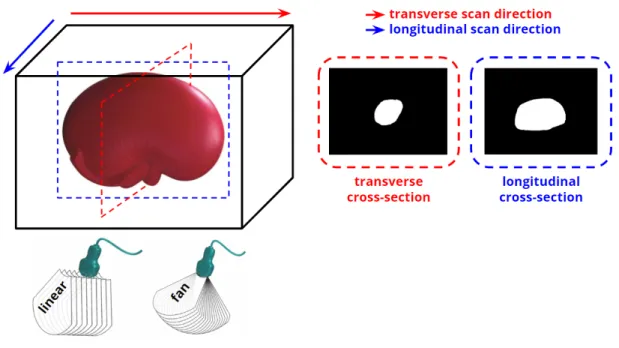
2.2.1 Hardware and Coordinate System . . . 45
2.2.3 Experimental Validation: Kidney Phantom . . . 48
2.2.4 Scanning Configurations . . . 49
2.2.5 Ground Truth Volume Measurements . . . 49
2.2.6 Renal Segmentation . . . 51
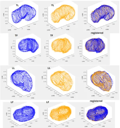
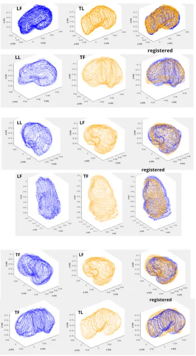
2.2.7 Inter and Intra Scan Volume Registration . . . 52
2.2.8 Statistical Analysis . . . 52
2.2.9 Uncertainty Mapping and Multi-Scan Fusion . . . 52
2.3 Results and Discussion . . . 55
2.3.1 Renal Segmentation . . . 55
2.3.2 Point Clouds and Meshes . . . 56
2.3.3 Inter and Intra Scan Registration . . . 57
2.3.4 Renal Volumes . . . 59
2.3.5 Multiscan Fusion . . . 61
2.4 Conclusions . . . 62
3 Ultrasound Probe Localization using 3D Maps of Superficial Vascu-lature 69 3.1 Introduction . . . 70
3.1.1 Superficial Vasculature: Background and Existing Imaging Modal-ities . . . 72
3.2 Proposed Method . . . 72
3.2.1 RGB-D Camera . . . 74
3.2.2 RGB-D SLAM (ORBSLAM2) . . . 75
3.2.3 Vascular Segmentation . . . 76
3.2.4 Bag of Words for Vascular Features . . . 77
3.3 Results and Discussion . . . 79
3.3.1 3D Maps of Superficial Vasculature and Accuracy of Localization 79 3.3.2 Affine Registration of 3D Vasculature Maps . . . 81
3.3.3 Patch Based Relocalization using 3D Vasculature Maps . . . . 84
4 2D Speed of Sound Mapping using Reflection Ultrasound
Tomogra-phy 89
4.1 Introduction . . . 90
4.2 Proposed Method . . . 92
4.2.1 Multilook Reflection Ultrasound Tomography . . . 93
4.2.2 Mathematical Formulation of the Inverse Problem . . . 94
4.2.3 Numerical Regularization . . . 97
4.2.4 Summary of the Inverse Problem . . . 99
4.2.5 Ultrasound Probe Localization and Calibration . . . 99
4.2.6 Effect of Pose Uncertainty and Reflector Uncertainty on Inversion106 4.2.7 Solver . . . 108
4.3 Results and Discussion . . . 108
4.3.1 Synthetic Inversions . . . 108
4.3.2 Effect of Aperture Size on Inversion . . . 110
4.3.3 Effect of Temporal Measurement Noise on Inversion . . . 111
4.3.4 Effect of Pose and Reflector Uncertainty on Inversion . . . 113
4.3.5 Spatial Resolution of the Multilook Framework . . . 117
4.3.6 Synthetic Anatomical Domain . . . 119
4.3.7 Straight Ray vs. Bent Ray Inversions . . . 121
4.3.8 Experimental Inversions . . . 124
4.4 Bulk Sound Speed Estimation . . . 127
4.5 3D Sound Speed Estimation . . . 128
4.6 Conclusions . . . 130
5 Conclusions and Future Work 135 5.1 A Vision for the Future . . . 135
5.2 Contributions, Conclusions and Future Work . . . 136
5.2.1 Ultrasound Probe Localization . . . 136
5.2.2 2D Image Segmentation . . . 137
5.2.4 2D Uncertainty Mapping . . . 139 5.3 A Final Word . . . 139
List of Figures
2-1 Intel Realsense D435i camera . . . 46 2-2 Coordinate systems associated with the D435i and ultrasound (US)
probe setup . . . 47 2-3 Preserved sheep kidney for ex vivo validation . . . 49 2-4 US scanning configurations for ex vivo validation . . . 50 2-5 Ellipsoidal method for determining kidney volumes from US images. . 51 2-6 Representative segmentations of kidney b-mode images . . . 56 2-7 Representative meshes/point clouds of reconstructed ex vivo sheep kidney 57 2-8 Intra-scan registration results . . . 58 2-9 Inter-scan registration results . . . 65 2-10 Volume estimates using freehand ultrasound scans (kidney 1 and
kid-ney 2) . . . 66 2-11 Ground truth trajectory (dashed) compared to estimate trajectory in
the xy plane (top) and xz plane (bottom) . . . 67 2-12 Multiple 3D point clouds of a lower lumbar spine phantom . . . 68 2-13 High fidelity 3D reconstruction of a lower lumbar spine phantom . . . 68 3-1 Vascular Mapping Framework . . . 73 3-2 NIR and depth feeds of the D415 camera at a resolution of 240 pixels
x 424 pixels and 30 fps . . . 74 3-3 Coordinate systems associated with Intel Realsense D415 camera . . . 75 3-4 Raw infrared image of the forearm (right) and segmented image (left)
3-5 Extracted features in a segmented vascular network during real-time
scanning of the forearm . . . 79
3-6 3D sub-map of the superficial vasculature of the human forearm (left) within a larger 3D map of the human arm/forearm . . . 80
3-7 Ground truth trajectory (dashed) compared to estimate trajectory in the xy plane (top) and xz plane (bottom). . . 81
3-8 Scanning protocol used to demonstrate affine registration . . . 82
3-9 Representative 3D maps of superficial forearm vasculature obtained using three different scanning trajectories . . . 83
3-10 Vascular point cloud registration for a given trajectory. . . 84
3-11 Vascular point cloud registration across trajectories. . . 85
3-12 Vascular patch relocalization for a given trajectory . . . 87
4-1 Multilook reflection tomography framework . . . 93
4-2 Formulation of sound speed inversion problem. . . 95
4-3 Extended effective aperture in a multilook framework. . . 98
4-4 Calibration setup for multilook reflection framework . . . 100
4-5 Travel times for the full SA dataset capture for a wire target in deion-ized water. . . 102
4-6 Representative calibration results for the multilook reflection tomog-raphy framework . . . 103
4-7 Comparison of the b-mode images obtained for a representative look of a wire target submerged in deionized water, housed within an alu-minum container. . . 104
4-8 Representative calibration results for the multilook reflection tomog-raphy framework . . . 105
4-9 Coordinate geometry for the multilook framework. . . 109
4-10 Sound speed inversions for the circular inclusion as a function of in-creasing effective aperture. . . 111
4-11 Sound speed inversions for the Gaussian inclusion as a function of increasing effective aperture. . . 112 4-12 Sound speed inversions for the circular inversion with a maximum look
angle of +/- 45 degrees as a function of increasing temporal noise. . . 113 4-13 Sound speed inversions for the Gaussian inversion with a maximum
look angle of +/- 45 degrees as a function of increasing temporal noise. 114 4-14 Sound speed inversions for the circular inclusion with maximum
tem-poral noise as a function of increasing aperture. . . 115 4-15 Sound speed inversions for the Gaussian inclusion with maximum
tem-poral noise as a function of increasing aperture. . . 116 4-16 Representation of the sound speed maps using a finite number of DCT
coefficients. . . 117 4-17 Representative modes of 2D cosine functions. . . 118 4-18 Effect of aperture size on the variance of the estimated slowness map. 119 4-19 Comparison of sound speed uncertainty for the Gaussian inclusion as
a function of aperture size. . . 120 4-20 Reconstruction of a checkerboard pattern as a function of aperture size. 121 4-21 Reconstruction of checkerboard patterns with maximum aperture. . . 122 4-22 High resolution MRI image of a human quadricep muscle from the
Visible Human Project. . . 123 4-23 Inversion results for human quadricep muscle. . . 124 4-24 Inversion results for the human quadricep muscle. . . 125 4-25 Sound speed inversions for the Gaussian inclusion as a function of
increasing effective aperture without the assumption of straight rays. 126 4-26 Sound speed inversions for the circular inclusion as a function of
in-creasing effective aperture without the assumption of straight rays. . 127 4-27 Experimental setup for validating the multilook framework. . . 128 4-28 Measured travel times for seven distinct looks of the hotdog + water
configuration. . . 129 4-29 Inversion results for the hotdog + water configuration. . . 130
4-30 Inversion results for the hotdog + water configuration. . . 131 4-31 Inversion results for the HMA + water configuration. . . 132 5-1 3D Speed of Sound Mapping. A Vision for the Future. . . 135
List of Tables
2.1 Inter and intra-scan registration results. The table reports the mean RMSE over 24 scans for both kidneys. The registration of point clouds was done using the Go-ICP algorithm. . . 59
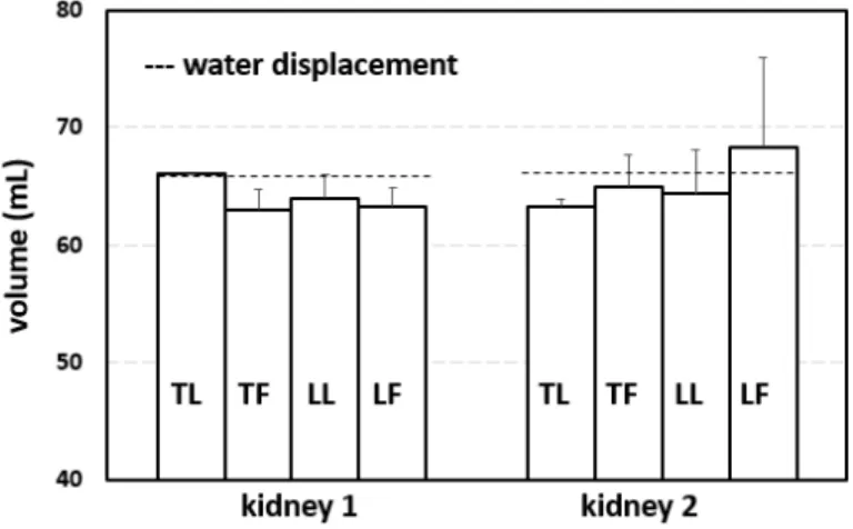
2.2 Volume estimates using freehand ultrasound scans (kidney 1). The mean ground truth value was obtained using water displacement (66.0 mL, 3 measurements). The mean volumes obtained using freehand scans were found to be 66.0 mL, 63.0 mL, 64.0 mL and 63.3 mL for TL, TF, LL and LF respectively (24 scans). The errors were 0.00 percent, -4.55 percent, -3.03 percent and -4.04 percent respectively with corresponding standard deviations of 0.00 mL, 1.73 mL, 2.00 mL and 1.53 mL. . . 60
2.3 Volume estimates using freehand ultrasound scans (kidney2). The mean ground truth value was obtained using water displacement (66.2 mL, 3 measurements). The mean volumes obtained using freehand scans were found to be 63.3 mL, 65.0 mL, 64.3 mL and 68.3 mL for TL, TF, LL and LF respectively (24 scans). The errors were -4.33 per-cent, -1.81 perper-cent, -2.82 percent and 3.22 percent respectively with corresponding standard deviations of 0.58 mL, 2.65 mL, 3.79 mL and 7.64 mL. . . 60
2.4 Volume comparisons across different techniques: freehand US, CT, wa-ter displacement, and the ellipsoidal method (across 24 scans). The mean error for freehand US across all scanning configurations was 2.90 percent for kidney 1 and 1.40 percent for kidney 2. The ellipsoidal method had errors of 12.90 percent and 9.13 percent; CT had an error of 4.54 percent. . . 61 3.1 Point cloud registration errors across 𝑇1, 𝑇2, and 𝑇3 for rigid affine
registration. The displayed values are averages of 4 samples for each configuration. . . 86 3.2 Point cloud registration errors across 𝑇1, 𝑇2, and 𝑇3 for patch
relocal-ization.The displayed values are averages of 4 samples for each config-uration. . . 86
Thesis Overview
This thesis presents a framework that uses a commercial ultrasound probe to generate accurate 3D organ property maps (specifically volume and sound speed) at the point of care.
Chapter 1 highlights the clinical motivation for using volumes and sound speed maps as relevant biomarkers. Both metrics have shown promise in staging and quanti-fying the progression of various diseases such as autosomal dominant polycystic kidney disease (ADPKD), non-alcoholic fatty liver disease (NAFLD), and breast cancer. The chapter also includes a rigorous and complete summary of existing techniques for ob-tained 3D organ property maps using magnetic resonance imaging (MRI), computed tomography (CT) and ultrasound (US). Finally, the chapter summarizes the current clinical need and the scope of the work being presented.
Chapter 2 summarizes the process of creating 3D structural volumes of organs using freehand ultrasound scans. Multiple low-cost sensors are fused in a Bayesian framework to localize the probe relative to its environment; the estimated poses are combined with the acquired 2D ultrasound images to create high fidelity point clouds and surface meshes. It also includes techniques for longitudinal registration (rigid and non-rigid) of acquired volumes. The method is tested on ex vivo sheep kidney with comparisons to water displacement and CT measurements. This chapter includes a detailed mathematical framework for estimating the uncertainty in the organ volumes. The uncertainty estimates are used to perform, what we call, "multi-scan" fusion i.e. multiple independently acquired estimates of property maps are combined to reduce the uncertainty of the final estimate.
Chapter 3 expands the localization framework of Chapter 2 to mitigate the effects of patient motion. Localizing an ultrasound probe relative to the environment results in errors that arise from voluntary and involuntary patient motion. This chapter proposes and validates a technique to use a patient’s vasculature network as stable fiducial markers. The method is tested and validated on volunteers, demonstrating its ability to create 3D maps of the superficial vasculature as well as its ability to
localize an ultrasound probe relative to this map. The chapter also includes a frame-work which allows sub-maps and full-maps of to be registered to one another for longitudinal monitoring.
Chapter 4 focuses on the use of localized ultrasound scans to estimate 2D sound speed maps. The techniques presented in Chapter 2 and 3 allow us to interrogate a domain of interest from arbitrary but known vantage points. By measuring the travel times from elements of a commercial ultrasound probe to strategic locations within the domain of interest, we are able to estimate the sound speed distribution within the domain. The method is rigorously validated in simulations and experiments, demonstrating its ability to produce accurate 2D SOS maps in a clinical setting. The chapter also includes a rigorous formulation for estimating the uncertainty in the predicted sound speed maps.
Finally, Chapter 5 summarizes the novel contributions of the thesis and highlights the shortcomings of the existing work. It also details the next steps involved in trans-lating the proposed technology into a clinical setting; it also includes a description of the existing code base.
Chapter 1
Background and Motivation
1.1
3D Sound Speed and Structural Maps as
Biomark-ers
3D organ property mapping has gained a considerable amount of interest in the re-cent years because of its superiority over its 2D counterpart. 3D images can provide clinicians with contextually accurate information that can greatly aide and inform diagnosis and treatment. For the most part, imaging modalities such as computed tomography (CT) and ultrasound (US) are designed to provide clinicians with 2D slices of 3D structures/property maps (e.g. the sagittal plane in a magnetic reso-nance image (MRI)). As a result, the burden of creating an implied 3D image or property map rests solely with the clinician. In doing so, the clinician has to rely on contextual clues within the 2D slices and/or prior anatomical knowledge. Even then, 2D information is often inadequate and does not provide clinicians with a com-plete understanding of the current state of the organ/tissue. The following are three motivating examples where 3D information becomes important and sometimes even necessary.
1.1.1
Chronic Kidney Disease (CKD)
Renal volume has been found to correlate well with glomerular filtration rate (GFR) [66][85]. The glomeruli, a cluster of capillaries found in the renal parenchyma, are re-sponsible for filtering waste from the blood and as such, are indicative of overall kidney health. Renal volume or more specifically, total kidney volume (TKV) is a valuable biomarker in diagnosing and tracking the progression of chronic kidney disease (CKD) [85][66]. TKV is also valuable in evaluating transplantations, nephrectomy, and ren-ovascular diseases [85][66][5]. TKV is also relevant in diagnosing and quantifying the progression of autosomal dominant polycystic kidney disease (ADPKD). ADPKD is an inherited disorder characterized by progressive kidney cyst formation and kidney enlargement. Over time, this leads to disruption of kidney function and ultimately kidney failure between the fifth and seventh decades of life in a majority of patients. Typically the disease is diagnosed by monitoring serum creatinine levels and GFR, but these are slow to change and generally do not show significant variability until the fourth or fifth decade of life; at this point, it is generally too late. TKV has been proposed as viable alternative because the kidney size is literally changing due to the development and growth of cysts. The Consortium for Radiologic Imaging Studies of Polycystic Kidney Disease (CRISP) conducted a longitudinal study of ADPKD patients; the study used magnetic resonance imaging (MRI) to determine whether change in TKV can be detected over a short time period and whether it is correlated with decline in kidney function [97]. Over a 3-year period, TKV increased by 204 mL (P <.001 vs. baseline) and total cyst volume increased by 218 mL (P <.001) in 210 patients. The correlation between change in TKV and cyst volume was r = 0.95 (P <.001) [97]. In addition, the study showed that cyst and kidney growth occur as a continuous, steady rate in most patients [97].
1.1.2
Non-Alcoholic Fatty Liver Disease (NAFLD)
Non-alcoholic fatty liver disease (NAFLD) is a chronic disease defined as the presence of hepatic steatosis (> 5 percent) in the absence of any known cause and minimal
alcohol use [8][81][110]. NAFLD is the most common liver disease with an estimated 1 billion patients globally and an estimated prevalence of 17 percent to 51 percent in the general population, with even higher rates in Western countries [9][81][110]. More specifically, in the United States, NAFLD afflicts roughly 45 percent of the population, and by 2020, NAFLD is projected to be the leading indicator and cause of liver transplantations in the world [8][81][110]. The spectrum of NAFLD is divided into two categories: (i) Simple steatosis (NAFL), which makes up 70 percent to 75 percent of cases, is defined by excess liver fat without inflammation. (ii) Steatohepatitis (NASH), which makes up 25 percent to 30 percent of cases, is defined by excess liver fat with inflammation and/or fibrosis [19][67]. In the case of NAFLD/NASH, the speed of sound within the liver parenchyma has the potential to serve as a robust and accurate biomarker. Because fat has a lower speed of sound than healthy liver tissue, any fat infiltration would become evident in the speed of sound distribution within the liver [40][50][58]. Multiple studies have been conducted to test the accuracy and validity of using speed of sound as a biomarker in this context [83]. Even in the later stages of the disease (NASH), when localized inflammation and fibrosis start to take effect, a spatial map of the longitudinal speed of sound distribution within the volume of the liver would greatly assist in identifying diseased regions of the organ, informing treatment options, and gaging the efficacy of existing treatment protocols.
1.1.3
Breast Cancer
Women with dense breasts have a higher risk of developing breast cancer than do those who have less dense parenchymas [80]. The density of breast tissue has been shown to have a strong correlation with the likelihood of developing breast cancer [11]. The ability to accurately, quickly, and non-invasively create 3D density maps of the breast tissue would greatly aide early diagnosis and intervention. In addition to density, the speed of sound within breast tissue also serves as a valuable biomarker in the detection of malignant tumors. Breast has a relatively low longitudinal speed of sound (< 1430 m/s) as it is composed primarily of adipose tissue. However, breast tumors or lesions are stiffer than adipose tissue and tend to cause increases in the
speed of sound [11]. Consequently, being able to map out the stiffness or speed of sound over entire volume of the breast can aide in the diagnosis and early detection of cancers. Given that nearly 1 in 8 women develop invasive breast cancer over the course of a lifetime (12 percent globally) with 3 million women in the United States alone [80], early detection and treatment is critical.
The above are a few examples of why 3D medical imaging, particularly in the space of organ volumes and speed of sound maps, provides clinicians with a greater level of insight into disease pathologies and organ health than do 2D images.
1.2
Existing Methods for 3D Organ Property
Map-ping (Volume and Sound Speed)
1.2.1
Computed Tomography (CT)
The term “computed tomography”, or CT, refers to a computerized x-ray imaging procedure in which a narrow beam of x-rays is aimed at a patient and quickly rotated around the body, producing signals that are processed by the machine’s computer to generate cross-sectional images—or “slices”—of the body. These slices are called tomographic images and contain more detailed information than conventional x-rays. Once a number of successive slices are collected by the machine’s computer, they can be digitally “stacked” together to form a three-dimensional image of the patient that allows for easier identification and location of basic structures as well as possible tumors or abnormalities. Much like in the case of magnetic resonance imaging (MRI) volumes, CT slices are obtained at known positions and orientations. As a result, the process of reconstructing volumes is less cumbersome than in the case of ultrasounds and a lot more accurate. Breiman et al. report the accuracy of CT scans to estimate the volumes of dog kidneys (ex vivo) and the human spleen before splenectomy. The mean percentage error of volume calculations using the sum-of-areas technique was 3.86 percent for eight dog kidneys, 3.59 percent for eight human spleens in vivo at 1 cm scan spacing, and 3.65 percent for the same human spleens [13]. Diaconu et al.
used CT imaging to estimate the orbital volumes of 12 cadaver eye orbits. Each orbit was dissected to isolate the extraocular muscles, fatty tissue, and globe. The empty bony orbital cavity was then filled with sculpting clay. The volumes of the muscle, fat, globe, and clay (i.e., bony orbital cavity) were then individually measured via water displacement. The CT-derived volumes, measured by manual segmentation, were compared to the direct measurements to determine validity [13]. The authors found that the CT estimates were within 95 percent of the water displacement values, thereby indicating the high level of accuracy of volumes obtained using CT imaging. Liu et al. used CT imaging to estimate the volumes of 24 bicuspids extracted for orthodontic purposes; these estimated volumes were compared to those obtained using water displacement. The estimated volumes were within 4-7 percent of the physical volumes [65].CT volumes are often used as ground truth measurements for in vivo applications and hence significant literature on comparisons between CT volumes and physical volumes (water displacement for example) are low in number.
In addition to structural volumes, CT is also capable of producing 2D and 3D property maps of organs. The principle of operation of a CT scanner lends itself well to the measurement of tissue attenuation. X-rays are preferentially absorbed or trans-mitted based on a region’s inherent attenuation. Li et al summarize these methods. In unenhanced CT, the brightness of a region directly translates to its attenuation. CT provides attenuation values in an absolute sense (Hounsfield units) or in a rela-tive sense (e.g. spleen vs liver). Voxel-based CT attenuation values are subject to be influenced by the contents in the dedicated voxel, so CT values may be influenced by other materials such as iron or glycogen [63]. Other sources of variations in attenua-tion values include CT scan settings (voltage, tube current, pitch, etc.) and patient parameters (BMI, iodinated contrast agents, etc.), all of which limit the reliability of unenhanced CT for quantitative measurement [63]. On the other hand, contrast-enhanced CT increases the sensitivity and specificty of attenuation values [63]. Recent advances in dual-energy CT (DECT) have introduced the ability to perform material decomposition, which has been shown to more accurately quantify hepatic steatosis and potentially permit fibrosis staging [63]. In DECT, the organ is imaged at two
different energy levels (typically 80 kVp and 140 kVp). Attenuation differences of tissue at different energies levels are a function of tissue composition, allowing for post-processing of images into “material decomposition images" [63]. Much like MRI, CT does not directly quantify the speed of sound in organs. However, attenuation, which is a measure of density and modulus, serves as a viable proxy for the speed of sound and a robust biomarker in the diagnosis of diseases.
1.2.2
Magnetic Resonance Imaging (MRI)
MRI is a non-invasive imaging technology that produces detailed anatomical images. It is often used for disease detection, diagnosis, and treatment monitoring. From a high level perspective, it works as follows: MRIs employ powerful magnets which produce a strong magnetic field that forces protons in the body to align with that field. When a radiofrequency current is then pulsed through the patient, the protons are stimulated, and spin out of equilibrium, straining against the pull of the magnetic field [78]. When the radiofrequency field is turned off, the MRI sensors are able to detect the energy released as the protons realign with the magnetic field. The time it takes for the protons to realign with the magnetic field, as well as the amount of energy released, changes depending on the environment and the chemical nature of the molecules [78]. Physicians are able to tell the difference between various types of tissues based on these magnetic properties [78]. MRI machines have the capability of steering the magnetic fields in such a way that uniformly spaced slices of the organ of interest can be acquired [see slice selection in [78]]. As a result, estimating the volume of an organ becomes a relatively straightforward problem: the known slice positions and orientations are combined with segmented images to create volumes [78]. Szczepaniak et al. conducted an extensive study to determine the accuracy of MRI in estimating pancreatic volume. Eight adult Yucatan mini-pigs were scanned using a gradient echo sequence, Fast Low Angle Shot with Volume Interpolated Breath Hold (FLASH VIBE), in three perpendicular planes. Szczepaniak et al. used parallel 3 mm thick contiguous slices, with a Field of View (FOV) = 400 mm x 250 mm, inter pulse time Tr = 2.35 ms, and echo time Te = 0.96 ms. In these mini-pigs, the measurements
of pancreatic volume by MRI and by water displacement were almost identical (R2 = 0.9867; p = 0.0001) [95]. Wu et al. used MRI to establish the effect of anabolic steroids on muscle and organ growth. The goal of the study was to measure individual muscle and organ volumes in the intact and castrated guinea pigs undergoing a 16-week treatment protocol by two well-documented anabolic steroids, testosterone and nandrolone, via implanted silastic capsules. High correlations between the in vivo MRI and postmortem dissection measurements were observed for shoulder muscle complex (R = 0.86), masseter (R = 0.79), temporalis (R = 0.95), neck muscle complex (R = 0.58), prostate gland and seminal vesicles (R = 0.98), and testis (R = 0.96) [105]. These results demonstrated that quantitative MRI using a standard clinical scanner provides accurate and sensitive measurement of individual muscle and organ volumes [105][86]. used MRI to estimate organ volumes in infants following sudden death syndrome and compare those to the autopsy results. There was a good agreement between virtual and real volumes for brain (mean difference: -0.03 percent (-13.6 to +7.1)), liver (+8.3 percent (-9.6 to +26.2)) and lungs (+5.5 percent (-26.6 to +37.6)). For kidneys, spleen and thymus, the MRI/autopsy volume ratio was close to 1 (kidney: 0.870.1; spleen: 0.990.17; thymus: 0.940.25) [86].
In addition to volumes, MRI is also capable of producing property maps of organs. As described earlier, these serve as valuable biomakers in tracking the onset and pro-gression of diseases. Li et al summarize the use of MRI in diagnosing NAFLD. A stark difference in the precession of protons in fat and water allows for the robust detection of fat in the liver [63]. Frequency- selective MRI, chemical-shift-encoded MRI, and MR spectroscopy are three techniques that exploit fat-water precession differences to assess fatty liver disease. These are briefly summarized below. Frequency selec-tion MRI applies a radiofrequency pulse to selectively excite or suppress fat/water signals. Fat saturation is a common option for many clinical imaging sequences, in-cluding most spin-echo and gradient-echo based sequences at 1.5 T and higher. With fat saturation, the images coincide with the water signal alone; without fat satura-tion, they represent the sum of fat and water signals. Therefore, hepatic fat may be assessed by comparing these two sets of images [63]. Chemical shift encoded MRI or
the Dixon method uses the time dependent phase-interference between fat and water signals to detect and quantify fat contnet. Because fat and water molecules precess at different frequencies, they undergo phase interference at predictable intervals. Fat and water signals cancel at out-of-phase (OP) and add at in-phase (IP) echo times. Due to this phenomenon, hepatic fat may be assessed by comparing sequential OP and IP images. In fatty liver disease, the OP images show relative signal loss due to signal cancellation. In normal liver, the OP and IP images have similar inten-sities [63]. Current state-of-the-art MR techniques for quantifying hepatic steatosis include confounder-corrected chemical-shift-encoded MRI, which can estimate the proton density fat fraction (PDFF). Unlike US and CT, which use surrogate mea-sures of fat in the form of altered echogenicity and attenuation, PDFF meamea-sures the fraction of MRI-visible protons bound to fat divided by all MRI-visible protons in the liver (fat and water) [63]. Using this technique, the liver signal on MRI is divided into water and fat signal components by acquiring gradient echoes at appropriately spaced echo times, so as to quantify the percentage of liver fat. Images are acquired with a low flip angle to minimize T1 bias and at multiple echo times to measure and correct for T2* decay. The signal model mathematically incorporates a multi-peak fat spectrum to address the multi-frequency interference effects of protons in fat [63]. Lastly, Magnetic Resonance Spectroscopy (MRS) bins protons signals as a function of frequency; frequency spikes are determined by the inherent composition of the vol-ume under examination [63]. The MR spectrum describes the intensity of MR signal as a function of precession frequency, with fat and water producing the most visible peaks. However, water occurs as a single peak and fat shows as multiple peaks due to its multiple chemical components [63] Finally, Magnetic Resonance Elastography (MRE). Magnetic resonance elastography (MRE) uses a modified phase-contrast MRI sequence and an external mechanical actuator to induce and non-invasively visualize propagating tissue shear waves. It estimates the degree of fibrosis throughout the liver by analyzing the resulting wavefield using a so-called inversion algorithm from which the magnitude of the complex shear modulus is computed [63]. While Li et al. focus their review on the use of MRI to determine fat percentages, the aforementioned
techniques represent state-of-art methods for quantifying organ properties. A full list of applications in the space of breast cancer diagnosis, chronic kidney disease etc. can be found in [68][17]. While these techniques do not directly measure the speed of sound in organ volumes, they provide quantitative property maps that track with speed of sound and disease pathology.
1.2.3
Ultrasound (US)
Unlike MRI or CT, reconstructing organ volumes using US imaging is a non-trivial task. In the case of MRI, the magnetic fields can be precisely controlled to acquire 2D slices in arbitrary but known positions and orientations. In the case of freehand ultrasound scans, there is tremendous variability in the positions and orientations of the transducer/probe; there is a need for a method to accurately track the pose (orientation and position) of the ultrasound probe. Huang et al. provide a compre-hensive review of real-time 3D US imaging technologies [49]. The main aspects of the paper are summarized for the reader. In order to create a 3D image from a set of 2D images, one needs the spatial position and orientation (collectively called pose) of each acquired image in a known coordinate system. This can be achieved by: i) using 2D US probes which are capable of producing 3D images or ii) augmenting conventional 1D US probes with sensors/devices that are capable of localizing it in a fixed and known coordinate system [49]. The widespread use of 2D arrays has been precluded by their high cost, limited field of view (FOV), and computational complexity [49]. In light of these limitations, much work has been done to augment conventional 1D US with sensors that are capable of localizing the probe in free space. Huang et al. classify these methods as those that use mechanical localizers (i.e. motorized scanners) and those that operate in a freehand fashion [49]. When mechanical localizers are used, the pose of the US probe is known at all times; this is not true in the case of freehand scans. To resolve this, researchers have resorted to the use of acoustic positioners, optical positioners, articulated arm positioners and magnetic field sensors [49]. The details of these methods are summarized in [49]. Broadly speaking, each of these methods relies on affixing a “tag” of some sort (i.e.
infrared tags, electromagnetic tags, etc.) onto the US probe and using an off-board device to track the location and orientation of this tag [49]. While these methods do localize US probes, they tend to suffer from a key drawback that precludes their use in clinical settings. The methods detailed in [49] localize the US probe with respect to a fixed world coordinate system. The localization process assumes that the US probe is moving in space while everything else is fixed i.e. there is no relative motion between the region being scanned (in our example, the patient forearm) and the US probe. This is a valid assumption for ex vivo studies or studies involving phantoms, but is incorrect in a clinical setting. Patients frequently move voluntarily (e.g. mov-ing the body) or involuntarily (e.g. breathmov-ing), and there is a need for a technique that can localize a US probe with respect to the patient’s body, despite the patient’s motion. Instead of relying on external tracking devices, ultrasound probe localization by using only sensors mounted to the probe has been investigated, sometimes involv-ing the aid of inertial measurement units (e.g. gyroscopes and accelerometers) for providing measurements in additional DoF or for refining estimates. For instance, in [46], structured lighting sources and a camera are mounted to the ultrasound probe. By tracking the light pattern projected onto the skin surface during ultrasound im-age acquisition, the probe tilt angle against the skin surface is determined. Tari et al. describes a probe tracking method that involves affixing a specialized strip with high-contrast markers to the patient’s body and moving the probe alongside the strip [88]. Probe motion is estimated by tracking the markers using a camera mounted to the probe. Since the marker strip needs to be prepared beforehand, this approach is only suitable for simple and pre-determined scan paths. Ultrasound probe local-ization by using only ultrasound images is also under active research [62][90][20][99]. In this approach, relative probe motion between two adjacent images is estimated by measuring local correlation (or decorrelation) of ultrasound speckle patterns between the images. With the presence of fully developed speckles, a correlation-displacement curve for the specific tissue under investigation could be measured, from which probe motion could be accurately estimated. Since only ultrasound images are used for the estimation, no spatial calibration is required between an additional positioning
de-vice and the ultrasound image plane. This approach, however, generally suffers from gradually increasing drifting error when it is iteratively applied to ultrasound image pairs along a sequence of images since the bias in each pose estimate accumulates. Attempts have been made to correct this drift by combining other sensing methods, such as optical tracking [48][47], electromagnetic tracking [61], and speckle tracking using additional ultrasound transducer arrays [47]. This method also relies on the existence of fully developed speckles to obtain 6-DoF motion estimates, so it tends to be inaccurate when applied on real tissue [47]. Overall, this approach is currently unable to provide tracking accuracy comparable to external motion sensors, so it is usually used only for qualitative, but not quantitative, volume imaging. Our lab has previously demonstrated the use of a single camera to localize a US probe with respect to the body [1]. Sun et al. proposed a method in which a single camera is rigidly affixed to a US probe. Artificial skin markers (e.g. speckle tattoos) are applied onto the patient’s body (e.g. abdomen for liver scans or lower back for renal scans) and the camera tracks and triangulates these features using monocular simultaneous localiza-tion and mapping (SLAM), thereby localizing itself relative to the body [1]. A more complete and thorough list of the existing methods to localize probes using on board sensors can be found at [1]. From an accuracy standpoint, 3D US imaging still falls short of the volume estimates obtained using MRI image stacks. In the case of the kidney, for example, most studies employ mathematical formulas, such as the ellipsoid formula, to calculate the estimated renal volume i.e. length x breadth x thickness x 0.52 [28]. However, this widely used formula yields highly discrepant results and has been found to consistently underestimate renal volumes when compared to 3D volumetric CT (10 percent) and MRI (25 percent) [5][107][2]. The accuracy of the formula depends on calculations based on measurements such as the maximum renal length, maximum cross-sectional area or varied measurements of the three axes of the kidney, following the assumption that the organ resembles an ellipse, but ignoring variances in the shape [14]. Several 3D US-based methods (methods that use 2D US arrays) have been used to improve the accuracy of renal volume measurements. One study estimated renal volumes in children with autosomal dominant polycystic
kid-ney disease (ADPKD). The three-dimensional ultrasound (3D US) ellipsoid method yielded a volume of 169 ± 105ml vs. MRI 206 ± 130 ml (p < 0.001), and the stacked contour volumetry method yielded a volume of 185 ± 110 ml vs. MRI 206 ± 130 ml (p < 0.001) [14]. 3D US has also been used for renal volume evaluation in normal neonates; the method yielded a volume of 27.14 ± 7.89 ml vs. MRI 36.8 ± 10.94 ml (p = 0.008) [55]. Manually segmented 3D US images estimated the mean renal volume in normal adults to be 192 ml vs. multi-slice CT 210 ml (p < 0.001) [12]. 3D US measured renal volumes in normal adult and patients with chronic renal disease yielded a mean value of 231ml vs. 2DUS 232ml (p > 0.05) [14]. Previous studies have shown that these methods are still prone to underestimation when compared to MRI and CT-based estimates. Sources of error include operator variation, patient motion, image registration, soft tissue deformation, probe scanning angle, etc. For the liver, Treece et al. conducted a freehand ultrasound scan of the human liver using an off board electromagnetic tracker and reported an error of 5 percent when compared to ground truth volume measurements (MRI). Fritschy et al. report the use of a mor-phometric method to calculate liver volumes using CT and ultrasound images and compare them to those obtained using ground truth water displacement; for ten ex vivo specimens, volumes obtained using CT matched ground truth values well (R = 0.994) while those obtained using US correlated less well (R = 0.915).
Unlike MRI and CT, quantitative ultrasound (QUS) is capable of estimating the speed of sound in the tissue under examination. Broadly speaking, this can be di-vided into two categories: bulk speed of sound (SOS) estimation and 2D SOS map-ping. Orztuk et al. provide a thorough and comprehensive overview of methods for estimating bulk SOS [81]. Both shear wave speed (current paradigm) and the longi-tudinal wave speed have similar mathematical relationships to the elastic properties of tissue. Various approaches to derive these have been studied on phantoms, animal models or excised human liver samples [6][21][40][50][56]. With most image-based methods of speed of sound estimation, characteristics of the B-mode image are ana-lyzed for brightness or sharpness (high frequency content) near the focal zone. The technical origins of this approach are based on the work of Burckhard et al. and
Wagner et al., who recognized the similarity between laser and ultrasound speckle, and were able to demonstrate analytically increased brightness and reduced speckle size in the focal region [102]. These insights have been taken advantage of in sev-eral settings involving speed of sound, for example, image quality improvement [75], aberration correction [79], as well as several efforts in liver steatosis estimation [58] or in general speed of sound measurements. In addition to speckle based analysis, other researchers have used seismology based methods [4], triangulation or biprisms [21][91], and tomographically determined phase shifts within the imaged area from different viewing angles [51].
A bulk estimate of SOS is advantageous, but does not provide clinicians with a whole organ/slice view. 2D SOS estimation falls into five categories: i) shear wave elastography ii) full waveform inversion (FWI) and iii) travel time tomography iv) deep learning and v) b-mode image/raw data based methods. The currently employed model for ultrasound shearwave elastography of soft tissue is that of a linear isotropic elastic material. While this does not account for non-linear effects, it is still useful for diagnostic purposes for most soft tissues, and can be relatively easily extended to include the viscoelastic based attenuation by employing a complex sound speed. The pressure wave (also known as p-wave, primary wave or longitudinal wave) is an acoustic wave used for ultrasound imaging, and travels at 1540 m/s on average in soft tissue. The shear wave (also known as s-wave, secondary wave or transverse wave) is measured indirectly in ultrasound elastography, using pressure waves, and is much slower. Ultrasound shear wave imaging, is the currently deployed state of the art [43][77][39]. Common methods of shear wave generation include acoustic radiation force (ARFI) and supersonic shear wave [10][74]. A mechanical shear wave is generated in the tissue and its propagation velocity is tracked using pressure waves. These methods however are limited to high end devices due to high power and probe requirements. They also generally suffer from low frame rates, long settling times, and high sensitivity to sonographer and subject motion.
Travel time tomography measures first arrival times between a set of known transmitter-receiver pairs or travel times between known transmitter-reflector-receiver
triads [33]. This travel time depends on the integral of slowness (reciprocal of the sound speed) along the the path which minimizes the travel times [29]. Sanabria et al. have demonstrated single-sided sound speed inversion with and without a reflector at the far end of the domain of interest [93][94]. While promising, these methods have two key shortcomings: 1) the methods assume that the acoustic ray paths stay relatively straight in soft-tissue i.e. there is no significant bending and 2) the meth-ods suffer from poor resolution in the direction parallel to the probe face. This is mitigated by the use of heavy regularization which in turn, reduces the accuracy of the results [93][94]. The limited resolution stems from the fact that commercial ul-trasound probes have a finite and relatively small probe face; this greatly limits the aperture that is available for estimating sound speed maps.
FWI, on the other hand, performs optimization on a tissue model in order to minimize the residual between the signals measured at known transmitter-receiver pairs and those obtained using physics-based wave propagation models [29]. This research is currently mostly focused on breast [44][76][27][63][92], and musculoskeletal [33][32] imaging, both showing promising results. Current implementations in actual tissue, however, require a full circumferential field of view, limiting them to small body parts. The need for a full circumferential field of view also precludes their use in clinical settings, where a single-sided imaging modality (i.e. handheld ultrasound probe) is used. The limited aperture in these instances makes the inversion unstable and inaccurate. Additionally, FWI-based methods are computationally expensive and sensitive to noise and choice of initial conditions [29].
With the emergence of deep learning, there have been attempts to reconstruct speed of sound maps based on the raw data alone. Feigin et al. have successfully demonstrated the use of plane-wave imaging and multi-layered deep convolutional neural networks (CNN) to estimate 2D sound speed maps in simulations and in in vivo and ex vivo experiments [30][31]. Park et al. have used CNNs and transfer learning to estimated 2D velocity maps using raw data [84] and Yang et al. have used deep learning to estimate velocity maps in seismic applications [106]. Deep learning methods, while effective and easily deployed, require an extensive and exhaustive
number of training samples. Given the lack of existing methods to produce accurate and robust speed of sound maps, the training data is restricted to synthetic maps or those obtained using simulations. The use of surrogates during training greatly limits the generality and accuracy of the trained networks, especially when dealing with physical data.
Lastly, there have been numerous studies that attempt to use image and raw data from commercial scanners to estimate 2D sound speed maps. Local sound speed estimators based on pulse-echo acquisition geometry include the crossed-beam method [57] the modified beam tracking method [18], registered virtual detectors [16] and ultrasound computed tomography in echo mode (CUTE) [52]. Methods that use image metrics are summarized in [81]. The primary drawback of these methods is their inability to resolve sound speeds to the levels needed for clinical utility [53].
1.3
Reflection Tomography in Non-Medical Fields
In abstraction, the problem of determining the underlying sound speed distribution using a set of acoustic transducers is directly analogous to the problem of determin-ing the velocity distributions in the seismic community. The length and time scales are different, but the core idea holds: given a set of 𝑁 sources and 𝑀 receivers on the surface of the earth, how does one use the acquired time traces and the known locations of the sources/receivers to estimate the underlying velocity distribution? In the seismic community, the sources produce acoustic waves using accurately timed explosions; these acoustic waves penetrate the surface and interact with the unknown medium. Refraction, diffraction, bending, and scattering produce echoes from strong interfaces. These echoes are continually received by the receivers on the surface. The goal is then to create an accurate map of the unknown domain and to also estimate the sound speed distribution. A comprehensive summary of the last decade of inversion tomography in the seismic community can be found in [104]. The principal prob-lem of these methods is well known. They require a good starting model since they look for a solution in the close neighborhood of the starting model. Since the error
energy function to be minimized in the course of a tomographic inversion may have many points with vanishing gradient, if the trial solution is too far from the global minimum, the method may stop the inversion process at any point where the error energy function does not change significantly. This is due, in part, to the limited illumination of the unknown domain when using a single-sided approach. Because the source-receivers are on the earth’s surface, there is a very limited number of ray crossings in the direction parallel to the surface. This is especially true when ray-bending is taken into account and the rays are concentrated in regions of high sound speed; the remainder of the discretized cells remain sparsely populated. The lack of constraints necessitates an initial guess that is close to the optimal value [103]. This particular problem has been overcome in multiple ways, including the development of global optimizers, simulated annealing, stochastic optimizers, anisotropic regularizers [103][104]. The state-of-the-art in seismic reflection travel time tomography, as ref-erenced in [104], have tackled the issues of ray bending, non-linear iterative solvers, global convergence and regularization, but continue to be hindered by the limited aperture of the acquisition setup.
Additionally, the field of ocean acoustic tomography has a rich and diverse history with a multitude of algorithms being used to estimate properties such as temperature. The technique relies on precisely measuring the time it takes sound signals to travel between two instruments, one an acoustic source and one a receiver, separated by ranges of 100–5000 km. If the locations of the instruments are known precisely, the measurement of time-of-flight can be used to infer the speed of sound, averaged over the acoustic path. Changes in the speed of sound are primarily caused by changes in the temperature of the ocean, hence the measurement of the travel times is equiv-alent to a measurement of temperature. A 1 degree Celsius change in temperature corresponds to about 4 m/s change in sound speed. A comprehensive review of these methods can be found in [70]. Much like clinical ultrasound scanners, ocean acoustic tomography is limited to single-sided data collection and hence direct analogs arise. In the ray approximation used as part of this framework, travel times are sensitive to medium changes only along the corresponding eigenrays [25]. Ray travel times are
robust in the presence of internal-wave-induced scattering at least partly because of Fermat’s principle, which states that to first order ray travel times are not affected by ray path changes [25]. In full generality, however, the ray paths are subject to bend-ing; in these cases there have been multiple works relating to the use of the eikonal solver, along with regularization to solve the non-linear inverse problem [54][89][25].
1.4
Scope of this Work
CT and MRI continue to be clinical standards for the spatial monitoring of organs and tissues. Both modalities benefit from high accuracy and resolution. Both meth-ods, however, suffer from limited portability, high-cost and long scan times. This limits their widespread use, especially in resource constrained settings or cases that necessitate frequent scanning. Ultrasound, on the other hand, is extremely portable and low-cost. With the advent of modern technology, ultrasound scanners can in-terface with phones and tablets and are priced as low as 3000 USD. They produce low-resolution images, but at a high frame rate; this allows for real-time monitoring and diagnosis. The two primary drawbacks of this modality are the fact that the images are largely qualitative and are prone to errors due to operator variability. To that end, the scope of this work is to develop a framework that allows clinicians to obtain quantitative, 3D property maps of organs using freehand ultrasound scans. The quantitative nature of the maps allows clinicians to move away from qualitative diagnoses and paves the way for the use of ultrasound as a point of care diagnos-tic tool; the 3D nature of the property maps overcomes the problems of scanning variability. While 2D sections of organs can be misinterpreted or misdiagnosed, a 3D map allows clinicians to understand the spatio-temporal behavior of the organ, thereby minimizing the associated errors.
First, within the space of 3D mapping, as detailed above, a considerable amount of work has been done to augment linear array transducers with low-cost sensors; these include cameras, IMUs, GPS, electromagnetic trackers, optical trackers, mechanical scanners etc. These methods are capable of localizing an ultrasound probe in space
and also creating 3D volumes of organs. They are, however, not able to effectively account for patient motion. Almost all of the existing methods rely on environmental fiducials to perform the localization. To that end we have demonstrated three novel ideas here: 1) freehand volumetric scans of large organs along with comparisons to CT and water displacement 2) the use of a patient’s existing superficial vascular network as localization landmarks and comparisons to ground-truth optical tracking and 3) the creation of a “multi-scan” fusion framework which propagates localization uncertainty to the underlying volume and allows clinicians to improve the recreated volume. Second, within the space of organ property mapping, this work focuses on the use of commercial ultrasound probes to estimate the sound speed within the underlying organ of interest. Again, considerable work has been done within this space; travel time tomography, full waveform inversion, deep learning and focusing methods have yielded promising results for 2D sound speed maps. Within the space of travel time tomography, ultrasound has drawn from techniques from seismic inversion and ocean acoustic tomography. The latter are fields in which data is collected in a single-sided fashion (sources and receivers on the same side of the domain). Unlike in the seismic and oceanographic fields, ultrasound tomography is greatly hampered by the probe’s limited aperture. Most commercial ultrasound probes have a face width between 2.5 to 3 cm with at most 256 piezoelectric elements. As a result, the domain of interest is not adequately illuminated, resulting in an under-constrained problem. Our novel contribution here is to extend the principles of reflection travel time tomography but allowing the unknown domain to be interrogated from multiple vantage points; this increases the effective aperture of the imaging system, leading to better inversions. We believe that these novel contributions form the basis of a framework that will eventually allow ultrasound probes to be used for quantitative diagnosis at the point of care.
1.5
Discussion and Conclusions
There is a need for a low-cost, portable, quantitative method for creating 3D property maps of organs at point of care. 3D property maps are capable of providing clinicians with a greater deal of insight into disease pathologies, which in turn, informs treatment options.
MRI and CT are advantageous in the fact that they offer high resolution, quanti-tative 2D slices and 3D volumes. The volumes can be obtained intrinsically, because the patient is confined to fixed geometry. Both techniques have proven invaluable in providing clinicians with non-invasive, quantitative 3D property maps that aide in diagnosing and treating diseases. Both methods, however, are time and resource in-tensive; they do not lend themselves to point of care, real-time applications. Moreover, CT has the drawback of using ionizing radiation. Both techniques also suffer from motion artifacts induced by patient movement. They also do not lend themselves to dynamic 3D property mapping, because both modalities are not real-time/dynamic. Quantitative ultrasound (QUS) has emerged as a viable alternative. US is in-expensive, portable, safe, fast and dynamic. 2D area arrays, while promising, are expensive and have a limited field of view. This precludes the analysis of large organ volumes. Considerable work has been done to augment linear arrays with sensors that are capable of localizing the probe in free space. These, however, require bulky and expensive equipment, line of sight, stationary subjects, artificial fiducial markers etc. These drawbacks impede a clinician’s workflow, precluding their widespread use. Considerable work has been done to extract meaningful 2D SOS information from commercial probes. Given the one-sided nature of the acquisition and the limited aperture of commercial probes, however, the problem remains inherently ill-posed and challenging.
In summary, the current need is a feedback-drive, inexpensive, portable, method for 3D organ property mapping at point of care.
Chapter 2
Organ Volume Estimation Using
Freehand Ultrasound Scans
2.1
Introduction
This chapter presents a framework in which a commercial ultrasound probe, equipped with multiple low-cost sensors, is localized in space and is used to reconstruct the surface and interior morphology of an organ. Specifically, the method is used to estimate the volume of the organ in concern. The chapter first presents a motivating example i.e. the need for accurately estimating organ volumes in a clinical setting. It then summarizes the existing methods for organ volume estimation, details the proposed framework and presents the salient results and conclusions.
2.1.1
Total Kidney Volume as Biomarker: A Motivating
Ex-ample
Renal volume has been found to correlate well with glomerular filtration rate (GFR) [85][66], the rate at which the glomeruli, a cluster of capillaries found in the renal parenchyma, filter serum from the blood, and a common clinical measure of over-all renal health. Renal volume or more specificover-ally, total kidney volume (TKV) is a valuable biomarker in diagnosing and tracking the progression of chronic kidney
disease (CKD) [85][66], and is relevant in the clinical settings of renal transplanta-tion, nephrectomy, and renovascular disease[85][66]. TKV is particularly relevant in diagnosing and quantifying the progression of autosomal dominant polycystic kidney disease (ADPKD). ADPKD is an inherited disorder characterized by progressive kid-ney cyst formation and kidkid-ney enlargement. Over time, this leads to disruption of kidney function and ultimately kidney failure between the fifth and seventh decades of life in a majority of patients [97]. Renal failure is diagnosed by monitoring serum creatinine levels and GFR, but these are slow to change and in ADPKD generally do not show significant variability until the fourth or fifth decade of life; at this point, it is generally too late. TKV has been proposed as viable alternative since the kidney size changes drastically due to the development and growth of cysts. The Consor-tium for Radiologic Imaging Studies of Polycystic Kidney Disease (CRISP) was a prospective longitudinal observational cohort study of ADPKD patients. The study used magnetic resonance imaging (MRI) to determine whether change in TKV can be detected over a short time period and whether it is correlated with a corresponding decline in kidney function [97]. Over a 3-year period, TKV increased by 204 mL (p <.001 vs. baseline) and total cyst volume increased by 218 mL (p <.001) in 210 patients. The correlation between change in TKV and cyst volume was r = 0.95 (p <.001) [97].
2.1.2
Existing Methods for Estimating Total Kidney Volume
Renal volume has been assessed in many experimental and clinical studies using different imaging approaches. Studies have been performed to determine the most accurate method for measuring renal volume, such as computed tomography (CT) and magnetic resonance imaging (MRI). Studies using MR and CT imaging have yielded promising results. These methods are based on the assumption that the voxel count method (the sum of all voxel volumes lying within the boundaries of the kidney) is the most accurate method to estimate renal volume, because it is independent of the underlying shape [73][85]. However, manually tracing the kidney contours in each acquired slice (stacked volumetry method) is time-consuming, inefficient, and
prone to error [73][85][24]. Furthermore, the ionizing radiation and potential contrast nephrotoxicity of CT, and cost and unavailability of MRI limit their use as a routine imaging tool for measuring kidney volume [73], especially in resource-constrained settings.
Ultrasound (US) is a portable, non-invasive, and low-cost tool for measuring renal volume. Presently this is accomplished with predictive formulas that use indirect measurements as inputs [22]. The ellipsoid formula to calculate estimated renal vol-ume is length x breadth x thickness x 0.52 [28]. This widely-used formula yields discrepant results and has been found to consistently underestimate renal volumes when compared to three-dimensional (3D) volumetric CT (10 percent) and MRI (25 percent) [5][2]. The accuracy of the formula depends on calculations based on mea-surements such as the maximum renal length, maximum cross-sectional area or varied measurements of the three axes of the kidney, following the assumption that the organ resembles an ellipse half-rotated about its long axis, a solid shape termed a prolate spheroid. However, the kidney is not a prolate spheroid and commonly varies in shape [14]. Several 3D US-based methods (methods that use two-dimensional (2D) US arrays to produce US volumes) have been used to improve the accuracy of renal volume measurements. One study estimated renal volumes in children with autoso-mal dominant polycystic kidney disease (ADPKD). The three-dimensional ultrasound (3D US) ellipsoid method yielded a volume of 169 ± 105ml vs. MRI 206 ± 130 ml (p < 0.001), and the stacked contour volumetry method yielded a volume of 185 ± 110 ml vs. MRI 206 ± 130 ml (p < 0.001) [14]. 3D US has also been used for renal volume evaluation in normal neonates; the method yielded a volume of 27.14 ± 7.89 ml vs. MRI 36.8 ± 10.94 ml (p = 0.008) [55]. A study by Brancaforte et al mea-sured the renal volume in normal adults. The study used manually segmented 3D US images and estimated the mean renal to be 192 ml vs. multi-slice CT 210 ml (p < 0.001) [12]. Kim et al used 3D US to measure renal volumes in normal adult and patients with chronic renal disease. They yielded a mean value of 231ml vs. 2DUS 232ml (p > 0.05) ([56]. Previous studies have shown current ultrasound methods are still prone to underestimation when compared with MRI and CT-based estimates.
There are many sources of error, including operator variation, patient motion, image registration, soft tissue deformation, and probe scanning angle [73]. In addition to consistently under-predicting volume, the widespread use of 3D US probes for renal volume estimation is precluded by their limited field of view (FOV), high cost, and computational complexity [49].
One final note: The above section presents the existing methods for estimating renal volumes; a lot of the techniques and imaging modalities are applicable to other organ systems as well.
2.1.3
Volume Estimation Using Freehand Ultrasound Scans
and Commercial Ultrasound Probes
Freehand ultrasound affords clinicians the ability to scan an organ of interest (e.g. kidneys) from variable orientations and locations. The caveat, however, is that be-cause of this variability, estimating organ volumes using freehand ultrasound scans is non-trivial. Each acquired US image must be accompanied by a corresponding location and orientation in a fixed, known frame of reference. Huang et al. provide a comprehensive review of real-time 3D ultrasound imaging technologies [49]. The main aspects of the paper are summarized for the reader. In order to create a 3D volume from a set of 2D images, one needs the spatial position and orientation (col-lectively called pose) of each acquired image in a known coordinate system. This can be achieved by: i) using 2D ultrasound probes which are capable of producing 3D images or ii) augmenting conventional 1D ultrasound probes with sensors/devices that are capable of localizing the probe in a fixed and known coordinate system [49]. Work has been done to augment conventional ultrasound probes with sensors capable of localizing them in free space. Huang et al. classify these methods as those that use mechanical localizers (motorized scanners) and those that operate in a freehand fashion [49]. When mechanical localizers are used, the pose of the ultrasound probe is known at all times; but mechanical localizers limit the range of motion for scan-ning. This is non-ideal in clinical settings and less preferred than freehand scans.
To enable freehand scanning while having knowledge of the probe’s pose, researchers have resorted to the use of acoustic positioners, optical positioners, articulated arm positioners, and (electro) magnetic field sensors [49]. The details of these methods are summarized in [49]. Broadly speaking, each of these methods relies on affixing a tag of some sort (infrared tags, electromagnetic tags etc.) onto the ultrasound probe and using an off-board device to track the location and orientation of this tag [49]. While these methods do localize ultrasound probes, they suffer from a few key drawbacks that preclude their use in clinical settings. First, the equipment associated with these methods tend to be bulky and expensive. Secondly, and more importantly, since a remote sensor does the tracking, there has to be a direct line of sight between the ultrasound probe and the sensor in question. This direct line of sight is not always possible due to a number of factors, such as but not limited to patient positioning and exam room setup.
Instead of relying on external tracking devices, ultrasound probe localization by using sensors mounted on the probe has been investigated, sometimes involving the use of inertial measurement units (e.g. gyroscopes and accelerometers) for providing measurements in additional degrees of freedom (DoF) or for refining estimates. For instance, in [46], structured lighting sources and a camera are mounted to the ultra-sound probe. By tracking the light pattern projected onto the skin surface during ultrasound image acquisition, the probe tilt angle against the skin surface is deter-mined. Tari et al. describes a probe tracking method that involves affixing a spe-cialized strip with high-contrast markers to the patient’s body and moving the probe alongside the strip. Probe motion is estimated by tracking the markers using a cam-era mounted to the probe. Since the marker strip needs to be prepared beforehand, this approach is only suitable for simple and pre-determined scan paths and requires the scan trajectory to closely follow the strip with little deviation. Ultrasound probe localization by using ultrasound images is also under active research [62][90][99][20]. In this approach, relative probe motion between two adjacent images is estimated by measuring local correlation (or decorrelation) of ultrasound speckle patterns between the images. With the presence of fully developed speckle, a correlation-displacement
curve for the specific tissue under investigation can be measured, from which probe motion could be accurately estimated. Since only ultrasound images are used for the estimation, no spatial calibration is required between an additional positioning device and the ultrasound image plane. This approach, however, generally suffers from gradually increasing error when it is iteratively applied to sequential ultrasound image pairs. The bias in each pose estimate accumulates over time, resulting in drift. Attempts have been made to correct this drift by combining other sensing methods, such as optical tracking [48], electromagnetic tracking [61], and speckle tracking using additional ultrasound transducer arrays [48]. This method also relies on the existence of fully developed speckles to obtain 6 degree of freedom (DoF) motion estimates, so it tends to be inaccurate when applied on real tissue [48]. Overall, this approach is currently unable to provide tracking accuracy comparable to external motion sensors, so it is usually used only for qualitative, but not quantitative, volume imaging.
Our lab has previously demonstrated the use of a single, low-cost camera to localize an ultrasound probe with respect to the body [1]. Sun et al. proposed a method in which a single camera is rigidly affixed to an ultrasound probe. Artificial skin markers (e.g. speckle tattoos) are applied onto the patient’s body and the camera tracks and triangulates these features using monocular simultaneous localization and mapping (SLAM), thereby localizing itself relative to the body [1]. SLAM is the process of simultaneously and iteratively creating a map of an unknown environment and localizing the sensor in the map [71][37][96]. The history of SLAM is long, diverse and rich. Fuentes-Pacheco et al. and Mur-Artal et al. provide concise reviews of existing and state-of-the art SLAM techniques [71][37][96]. A complete survey of visual SLAM algorithms from 2010 to 2016 can be found in [96] and a complete survey of existing methods to localize ultrasound probes using on-board sensors can be found in [1].
We propose a method in which a low-cost RGB-D (red/blue/green/depth) camera and inertial measurement unit (IMU) are affixed to a conventional ultrasound probe. The method is capable of localizing the ultrasound probe with respect to the patient’s body. It allows for freehand scans with little restrictions on the size of the region being