1S-2S Spectroscopy of Trapped Hydrogen: The
Cold Collision Frequency Shift and Studies of BEC
by
Thomas Charles Killian
Submitted to the Department of Physics
in partial fulfillment of the requirements for the degree of
Doctor of Philosophy
at the
MASSACHUSETTS INSTITUTE OF TECHNOLOGY
February 1999
©
Massachusetts Institute of Technology 1999. All rights reserved.
A uthor ...
...
Certified by...
C ertified by ...
. .... ...Department of Physics
January 11, 1999
...Thomas J.
eytak
Professor o
hysics
Thesis Supervisor
Dani'i Kleppner
Lester Wolfe Professor of Physics
Thesis Supervisor
aI Accepted by ... MASSAEHUSETTS INSTITUTE gMOFTECHNO -.. I ...P . . . ...
.- ... .--T! mas J.
reytak
n, Department of Physics Graduate ommittee
1S-2S Spectroscopy of Trapped Hydrogen: The Cold
Collision Frequency Shift and Studies of BEC
by
Thomas Charles Killian
Submitted to the Department of Physics on January 11, 1999, in partial fulfillment of the
requirements for the degree of Doctor of Philosophy
Abstract
The cold collision frequency shift of the 1S-2S two-photon transition is studied in trapped spin-polarized atomic hydrogen at submillikelvin temperatures. This effect is the low temperature manifestation of the pressure shift and broadening familiar from spectroscopy at normal temperatures and pressures. We find the shift is given
by Avs-2s= -3.8 ± 0.8 x 10⁻¹⁰ n Hz cm3, where n is the sample density.
Theory is developed to express the shift in terms of the mean field interaction energy due to collisions and thus relate it to the s-wave triplet scattering lengths,
ais-is and aIs-2s. From this we derive aIs-2s = -1.4 ± 0.3 nm, which is in fair
agreement with a recent calculation.
1S-2S spectroscopy is a valuable probe of the density, temperature, and
atom-atom interactions in the trapped sample, especially in the regime of Bose-Einstein condensation (BEC). We describe properties of the condensate and how they are determined from the 1S-2S spectrum.
Thesis Supervisor: Thomas J. Greytak Title: Professor of Physics
Thesis Supervisor: Daniel Kleppner Title: Lester Wolfe Professor of Physics
Acknowledgments
Graduate school has been the best time of my life and I owe that to Amy Salzhauer. She always shares my excitement when things go well and is ready with a reassuring smile when progress seems slow or nonexistent. She has a talent for getting me out of the lab to enjoy the rest of life, and my experience at MIT has been richer because I have had someone with which to share it.
For as long as I can remember my parents have encouraged me to ask questions, take risks, and explore the world around me, and those lessons have served me well.
My family may not have understood why I spent the last five years staying up all
night working in the lab, but they were always supportive. Thanks!
I couldn't have asked for better advisors than Tom Greytak and Dan Kleppner.
They give their students the freedom to grow and take on challenges, and manage to encourage hard work without forgetting that above all, physics is fun.
In an experiment like this one, nothing gets done unless people can work together as a team, and this thesis wouldn't exist without the help of others in the lab.
I have learned a tremendous amount from working with Dale Fried, and I feel safe in saying that with him more than anyone else, I share feelings of great satisfaction and joy (and relief!) from finally seeing the experiment deliver on its promises.
Lorenz Willmann brought experience, a good sense of humor, and a passion for rigorous data analysis to the experiment - all of which were desperately needed. It is always a pleasure to work with him, even when learning about the subtleties of chi-squared.
I am envious of the younger graduate students, Dave Landhuis and Stephen Moss,
because I am sure they will accomplish and learn amazing things in the next few years. It is hard to leave something that has absorbed so much of my sweat and tears, but it is made much easier by the talent and remarkable good nature of the people who will take care of it.
I would have been lost in the lab if Claudio Cesar hadn't been here when I arrived.
process.
It has been a privilege to work and share an office with Adam Polcyn. I have never met anyone with a better disposition or more patience, and with all the phone
messages he took for me, I am sure I tested the latter!
Some of the most rewarding experiences I had at MIT have been working with undergraduates. In particular I value my friendships with Jonathan Goldman and
Sourav Mandal and the chance I had to watch them learn about physics.
I also thank Ian Applebaum for help with numerical computations and Professors
Contents
1 Introduction
2 Overview of Cryogenic Trapping and Cooling of Atomic Hydrogen
2.1 Background . . . . 2.2 Trapping Low Field Seeking Hydrogen Atoms . . . . . 2.2.1 M agnetic Trap . . . . 2.2.2 Forming Atomic Hydrogen in a Radio Frequency
2.2.3 Spin Polarization . . . . 2.2.4 Loss Processes and Gas-Surface Equilibrium . .
2.3 Evaporative Cooling . . . .
2.4 Forced Evaporative Cooling . . . . 2.4.1 Magnetic Field Saddlepoint Evaporation . . . .
2.4.2 Radio-Frequency Evaporation . . . .
2.5 Probing the Trapped Gas . . . .
2.5.1 Bolometric Temperature Measurement . . . . .
2.5.2 Bolometric Density Measurement . . . .
3 Overview of 1S-2S Spectroscopy in a Trap, 3.1 Background ... ...
3.2 Two-Photon Excitation . . . . 3.3 Detection Scheme . . . .
3.4 Microchannel Plate Photon Counter . . . .
3.5 Laser System . . . . . . . . 18 . . . . 20 . . . . 20 Discharge . . 22 . . . . 23 . . . . 24 . . . . 25 . . . . 27 . . . . 28 . . . . 30 . . . . 30 . . . . 31 . . . . 32 35 35 36 37 40 41 15 18
3.6 Photoexcitation Spectrum . . . .4
4 Formal Description of 1S-2S Two-Photon Spectroscopy 46 4.1 15-2S Two-Photon Transition Theory . . . . 46
4.1.1 Physical System and Interaction . . . . 46
4.1.2 Excitation Hamiltonian . . . . 47
4.2 Doppler-Sensitive Excitation . . . . 50
4.3 Doppler-Free Excitation: Simple Lineshapes . . . . 53
4.3.1 Atoms Nearly at Rest . . . . 53
4.3.2 Atoms in Motion: Time-of-Flight Lineshape . . . . 54
4.4 Doppler-Free Excitation: Numerical Simulation of Complicated Line-shap es . . . . 60
4.4.1 Effective Two-Level Hamiltonian and Evolution of the Single Atom Density Matrix . . . . 61
4.4.2 Cold Collision Frequency Shift . . . . 62
4.4.3 Additional Sources of Spectral Broadening . . . . 63
4.4.4 Numerical Calculation of the Time of Flight Lineshape . . . . 66
4.4.5 Coherence Effects . . . . 68
5 Cold Collision Frequency Shift: Observations 72 5.1 D ata . . . .. . . . .. . . . . 72
5.1.1 Experimental Procedure . . . . 72
5.1.2 D ata Analysis . . . . 74
5.1.3 Inhomogeneous Broadening and Shift . . . . 76
5.1.4 Systematic Uncertainties . . . . 77
5.1.5 Measured Value of x . . . . 78
5.2 The 15-25 S-Wave Triplet Scattering Length . . . . 79
5.2.1 Experimental Value of the 1S-2S Scattering Length . . . . 79
5.2.2 Comparison with Theory . . . . 80
5.3 Using the Cold Collision Frequency Shift as a Probe of the Trapped Gas 80 5.3.1 Noncondensed Gas . . . . 80
5.3.2 Bose-Einstein Condensation . . . . 83
6 Cold Collision Frequency Shift: Mean Field Theory 84 6.1 Mean Field Description for a Spatially Homogeneous System . . . . . 86
6.1.1 State Vectors . . . . 87
6.1.2 Hamiltonian and Mean Field Energies . . . . 89
6.1.3 D iscussion . . . . 91
6.2 Mean Field Description for a Bose Condensed Gas in a Magnetic Trap 93 6.2.1 System before Excitation . . . . 94
6.2.2 System after Excitation . . . . 95
6.2.3 D iscussion . . . . 98
6.3 Cold Collision Frequency Shift for an Arbitrary System . . . . 102
6.3.1 Sum Rule for the Mean Frequency Shift in the Spectrum . . . 102
6.4 Conclusion . . . 108
7 Spectroscopic Studies of a Quantum Degenerate Hydrogen Gas 110 7.1 Spectroscopic Signature of Bose-Einstein Condensation . . . 111
7.2 Doppler-Free Spectrum of the Condensate . . . . 112
7.3 Condensate Fraction . . . . 113
7.3.1 Theoretical Limit of the Condensate Fraction in Hydrogen . . 113
7.3.2 Spectroscopic Determination of the Condensate Fraction . . . 114
7.3.3 Determination of the Condensate Fraction from the Peak Shift in the Doppler-Free Spectrum . . . . 119
7.3.4 Implications of the Measurement of the Condensate Fraction . 119 7.4 Phase Diagram . . . 122
7.5 Spectrum of the Normal Fraction in the Degenerate Regime . . . 123
7.6 1S-2S Spectroscopy as a Probe of BEC . . . 125
8 Future Prospects 126 A High Resolution Spectroscopy 129 A.1 Best Achieved Resolution . . . 129
A.1.1 Time-of-Flight Broadened Lines . . . . 129
A.1.2 Coherence Effects . . . . 131
A.2 Laser Frequency Stability Limitations . . . . 131
A.2.1 Reference Cavity Shift with Light Power . . . . 131
A.2.2 Doppler-Shifts Along the Beam Path . . . . 134
A.3 Prospects for Improving the Frequency Stability . . . . 137
B 1S-2S Spectroscopy Appendix 138 B.1 Effective Two-Level Hamiltonian . . . . 138
B.2 Numerical Calculation of the Spectrum . . . . 141
C Boltzmann Transport Equation Derivation of the Cold Collision Fre-quency Shift 145 C.1 Evolution of the Single Atom Density Matrix . . . . 145
C.2 Quantum Boltzmann Transport Equation . . . . 147
C.3 Application to the 1S-2S Transition in Trapped Hydrogen . . . . 147
C .4 D iscussion . . . . 148
D Details of the Mean Field Theory Calculation of the Cold Collision Frequency Shift 150 D.1 Correlation Functions for a Homogeneous System . . . . 150
D.2 Interaction Energy for a Homogeneous System before Excitation . . . 152
D.3 Interaction Energy for a Homogeneous System after Excitation . . . . 152
D.4 Derivation of the Energy Functional for the Excited State of a Con-densed Gas in a Trap . . . . 155
D.5 Details of Elements of the Proof of the Sum Rule for the Mean Fre-quency of the Spectrum for an Arbitrary System . . . . 157
E 130Te 2 Reference Spectroscopy 161 E .1 Introduction . . . . 161
E.2 Saturated Absorption Spectroscopy . . . . 163
E.2.2 1S-2S F = 1 Reference Transition, i2 . . . . 165
E.3 Systematics of i2 Frequency Stability . . . . 167
E.3.1 Temperature . . . . 167
E.3.2 Column Density . . . . 168
E.3.3 Reliability and Cell to Cell Variation . . . . 168
List of Figures
2-1 Hyperfine structure of the iS ground state of hydrogen in a magnetic field . . . . 19
2-2 Overview of the trapping apparatus . . . . 21
2-3 Diagram of the discharge and cell top . . . . 23
2-4 Schematic of the magnetic trap and hydrogen cloud shortly after load-ing the trap ... ... 26 2-5 Time between collisions, T = 1/na'iiv/2 for various hydrogen densities
and tem peratures . . . . 27 2-6 Zeeman diagram of IS F = 1 states in low magnetic fields showing the
transitions driven for RF evaporation . . . . 29 2-7 Bolometric determination of the sample temperature . . . . 31 2-8 Decay of a trapped hydrogen sample . . . . 32 3-1 Level scheme for 1S-2S spectroscopy of magnetically trapped atomic
hydrogen... ... 37
3-2 Excitation and detection . . . . 38 3-3 Typical timing sequence for 15-2S excitation and detection . . . . 39
3-4 Laser system for 1S-2S spectroscopy of trapped atomic hydrogen . . 41
3-5 Composite 15-25 two-photon spectrum of trapped hydrogen . . . . . 45 4-1 Doppler-sensitive excitation spectrum of a sample held at a trap depth
of 280 p K . . . . 52
4-2 Cross sections of the laser beam and the trajectory of an atom in the x - y plane . . . . 55
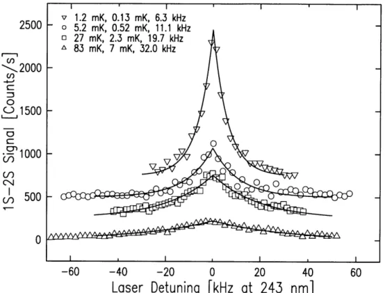
4-3 Typical Doppler-free spectra showing the dependence of linewidth on sam ple tem perature . . . . 58
4-4 Doppler-free spectra from cold, low density samples: 1/e half linewidths and inferred temperatures. . . . . 59 4-5 Probability for excitation to the 2S state for atoms which start outside
the laser beam and make one pass through the beam with zero impact param eter . . . . 66
4-6 Contribution to the excitation rate from all the atoms with a given atomic velocity in the laser beam, for various detunings from resonance 67 4-7 Numerical calculation of the probability for excitation to the 2S state
after a 1 m s laser pulse . . . . 69
4-8 Spectrum of a 275 pK sample showing coherence sidebands . . . . 70 5-1 Doppler-free spectra of a 120 pK sample with an initial peak sample
density of no = 5.0 x 10¹³ CM-3 . . . . 73
5-2 Analysis of spectra from a 120 [tK sample with an initial density of 6.6 x 1013 cm -3 . . . . 75 5-3 The frequency shift parameter X, determined as described in the text
for various trap configurations . . . . 78
5-4 Spectra of a 55 [pK sample (trap depth = 350 pK) with initial peak
sample density of between (1 ~ 2) x 10 CM~3 . . . . . . . . 81 6-1 Doppler-free spectra of noncondensed trapped hydrogen, showing the
cold collision frequency shift . . . . 85 6-2 Probability distributions of the number of atoms in the 2S state for a
total of 10 7 atoms and various fractions of atoms excited . . . . 89
6-3 1S-2S energy level diagram for a noncondensed, homogeneous sample,
showing the density-dependent level shift which gives rise to the cold collision frequency shift . . . . 92
6-4 Radial potentials and single particle wave functions for IS atoms in the condensate and 2S atoms trapped in the condensate interaction well 96
6-5 Theoretical Doppler-free spectrum of a condensate at T = 0 in a
three-dimensional harmonic trap . . . 100
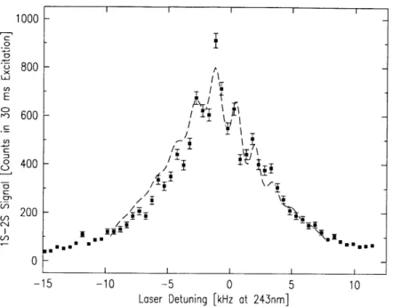
6-6 Doppler-free spectrum of a condensate: comparison of theory and ex-perim ent . . . 101
6-7 Graphical depiction of the sum rule . . . 103
6-8 Excitation of the system to excited state ivi) . . . 105
7-1 Composite 1S-2S two-photon spectrum of trapped hydrogen . . . 111
7-2 Typical laser and sample dimensions at the BEC transition . . . 115
7-3 Doppler-free spectra of normal fraction and condensate . . . 117
7-4 Spectroscopic determination of the condensate fraction . . . 118
7-5 Time evolution of the Doppler-free spectrum of a single condensate . 121 7-6 BEC phase diagram of hydrogen and a typical evaporative cooling path 123 7-7 Doppler-free spectrum of the normal fraction immediately after the end of the forced evaporation . . . 124
A-i Spectroscopy of cold (<40 piK) low density (<1013 cm-3) hydrogen . 130 A-2 Spectra showing motional sidebands . . . 132
A-3 Reference cavity transmitted power as measured by the FND-100Q photodiode/amplifier circuit . . . 133
A-4 Response of the reference cavity mode frequency to a sudden change in light level . . . 134
A-5 Schematic of the Doppler servo system . . . 135
A-6 Beatnote of Doppler servo system . . . 136
B-i Energy diagram for radial motion of an atom in the magnetic trap including the centrifugal potential, L2/2mr2 . . . . 142
E-i Doppler-sensitive and saturated absorption spectrum of 130Te 2 . . . . 162
E-2 Components of the laser system which are important for Tellurium spectroscopy... ... 164
E-3 Saturated absorption spectrum near 1/4 of the hydrogen 1S-2S F = 1
transition . . . . 165
E-4 High resolution saturated absorption spectrum of the 12 line in 1 30Te2 166 E-5 Temperature dependence of the frequency of the i2 line in 1 30Te 2 at saturated vapor pressure . . . . 167
E-6 Absorption on the center of the Doppler-broadened line 1284 . . . . . 169
E-7 Frequency of i2 plotted against linewidth . . . . 169
E-8 Linewidth of i2 versus oven temperature . . . . 170
List of Tables
Chapter 1
Introduction
Spectroscopy of atomic hydrogen has contributed to some of the major advances in physics in the twentieth century. Bohr's model to explain the hydrogenic electronic spectrum [1] was the bridge from classical to quantum mechanics. The fine structure splitting of the Balmer-alpha 2P-3S,3D transition led Sommerfeld to incorporate relativity in the description of the atom [2], a program which was continued by Dirac with his relativistic quantum theory [3]. Rabi's measurement of the ground state hyperfine structure [4, 5] suggested the existence of the anomalous electron magnetic moment. That work, along with Lamb's discovery of the 2S Lamb shift [6, 7], spurred the development of quantum electro-dynamics.
Today, hydrogen spectroscopy continues to occupy a prominent position in physics research, and there is particular interest in the two-photon 1S-2S transition because of its narrow natural linewidth, 1.31 Hz, at a resonance frequency of 2.46 x 10¹⁵ Hz. The 1S-2S transition, excited in an atomic beam, is part of the most precise measure-ment of the IS Lamb shift, which now stretches our understanding of the structure of the proton and quantum chromodynamics[8]. The transition is also important for metrology and fundamental physical measurements. It has been suggested as a fre-quency reference[9], and is used in the most precise determination of the Rydberg constant[9].
This thesis describes new applications for 15-2S hydrogen spectroscopy. We study H-H interactions in submillikelvin, magnetically trapped hydrogen[10] through the
cold collision frequency shift of the transition frequency [11, 12]. In addition, we show how 1S-2S spectroscopy and the cold collision frequency shift can be used to investigate Bose-Einstein condensation (BEC) in hydrogen[13].
The cold collision frequency shift is the low temperature manifestation of the pressure shift and broadening familiar from spectroscopy at normal temperatures and pressures [14]. In cold collisions, the temperature is so low that only a single partial wave contributes to atom-atom scattering. Collisional frequency shifts in this regime have been studied in the microwave region because they limit the accuracy of the cryogenic hydrogen maser [15] and atomic fountain clocks based on cesium[16, 17, 18]. The 1S-2S observations described here extend this research from the microwave to the optical region.
In hydrogen, the shift can be related to the s-wave elastic triplet scattering lengths for 1S-2S and IS-IS collisions, as-2s and ais-is. The IS-IS scattering length is known accurately from theory. To our knowledge these results constitute the first measurement of a scattering length involving an excited state, and it tests the under-standing of H-H molecular potentials.
The theory for the cold collision frequency shift in masers and fountain clocks has been thoroughly developed [15], but this theory strictly applies only to a homogeneous noncondensed system. The extension to an inhomogeneous gas, and to BEC, is not trivial. The frequency shift is sensitive to atom-atom spatial correlations, and raises interesting new questions about the state of the system after excitation.
The study of dilute degenerate quantum gases has captured the attention of the physics community and the popular press since the condensation of rubidium [19], sodium [20], and lithium [21, 22] in 1995. The observation of BEC in hydrogen capped a 22-year research effort, and 1S-2S spectroscopy was an essential tool for detecting the phase transition. High resolution spectroscopy is a new method for studying BEC and it opens another window into this exciting phenomenon.
The techniques for magnetically trapping and cooling hydrogen are discussed in Chap. 2. The experimental details of 1S-2S spectroscopy are described in Chap. 3. Chapter 4 provides a theoretical description of two-photon excitation in a trap and
presents spectra observed under various experimental conditions.
Chapter 5 describes the data and analysis for the cold collision frequency shift measurements, and Chap. 6 discusses the theory for the shift, which is necessary for relating the shift to the s-wave scattering lengths. Chapter 7 discusses some of the
BEC measurements that can be extracted from the 1S-2S spectrum, and Chap. 8
describes future prospects for the experiment.
Appendix A describes the current limitations and future potential of high reso-lution 1S-2S spectroscopy in the magnetic trap. Appendices B-D provide detailed derivations of many of the calculated results presented in the bulk of the thesis, and
App. E describes the "0Te2 reference spectrometer used to locate the frequency of
the 1S-2S transition.
This work should be viewed as a companion to D. Fried's Ph.D. thesis [23], "Bose-Einstein Condensation of Atomic Hydrogen," which discusses the condensate data and properties in much greater detail. This experiment is a group effort, and the emphasis here is on describing how the 1S - 2S transition is used to study the trapped gas,
Chapter 2
Overview of Cryogenic Trapping
and Cooling of Atomic Hydrogen
The study of magnetically trapped atomic hydrogen has been motivated by the pur-suit of BEC, a phase transition to a state in which a macroscopic number of atoms occupies the lowest energy level of the system. The transition occurs at low temper-atures and high densities when noA ~ 2.612, where no is the peak sample density,
AT =h/ /2w7mkBT is the thermal de Broglie wavelength, and noA4 is the peak phase space density in the sample.
The techniques for trapping and cooling hydrogen have been discussed extensively in the literature (references given below), and also in the Ph.D. thesis of J. Doyle [24]. This chapter gives an overview of this aspect of the experiment and a bit of historical background.
2.1
Background
The study of gaseous atomic hydrogen in the quantum regime can be traced back to Hecht[25], who in 1959 pointed out that in a strong magnetic field the system would remain a gas to T = 0 and, at low enough temperatures, might display the effects of quantum degeneracy and superfluidity. There was little initial interest, but experimental work started in earnest in the 1970's after further details were worked
I I I I I I
0
0.12
0.24
0.36
Magnetic Field [Tesla]
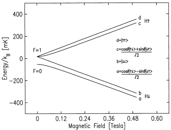
Figure 2-1: Hyperfine structure of the IS ground state of hydrogen in a magnetic field. The symbol
Itt)
denotes the state with the electron spin up, me = +1/2, and the proton spin up, mp = +1/2, etc. The mixing angle is defined by tan(20) =A/h('ye + 'yp)B = .0506/B, where A/h is the zero field hyperfine splitting, and Ke
are 7, are the electron and proton gyromagnetic ratios, respectively. In high field (B > 0.05 T), the electron and proton spins couple to the magnetic field; in low field
the hyperfine coupling dominates. Electron spin up atoms (Ht) are pulled towards the magnetic field minimum, while the electron spin down atoms (H) are pulled towards the maximum of the field. According to convention, states are labelled a through d in order of increasing energy.
out by Stwalley and Nosanow[26] and others [27]. To stabilize the system against molecular recombination, a magnetic field is required to spatially separate atoms with different electron spins. This greatly suppresses the exothermic reaction H + H
=> H2 + 4.6 eV, because electron spin-polarized atoms interact through the repulsive
triplet molecular potential[28, 29].
Atomic hydrogen interacts with a magnetic field through the well known Zeeman effect [30]. The orientation of an atom's spin tends to follow the field adiabatically due to the spin angular momentum, so the magnetic potential, U = -p - B, reduces to a function of the magnitude of the field, as shown in Fig. 2-1. Atoms with their
400
2001
E m wD -0-200
d cHt -C d=ltt> F=1 c=cos6It4>+sin8I4t F=O a=cosOlt4>-sinelJt b a-400
0.48
0.60
> >electron spin down (H4, states a and b) are pulled towards a magnetic field maximum. Atoms with their electron spin up (HT, states c and d) are pulled towards a magnetic field minimum.
H4 atoms were magnetically stabilized by Silvera and Walraven [31] in 1979. The sample was confined at 300 mK in a liquid 4He coated cell in fields of up to 7 T. In
a similar apparatus, nuclear polarization was demonstrated in 1981 when the group of Greytak and Kleppner produced a sample of b state atoms [32].
Bose condensing high field seeking atoms proved impossible in these experiments because the trapped H4 atoms were always in thermal and diffusive contact with containment walls. This limited the temperature to greater than about 100 mK and three body recombination limited the sample densities to less than ~ 1018 cm-3 [33],
below the BEC critical density. Containment walls were essential because Maxwell's equations forbid the existence of a static magnetic field maximum in free space.
Hess [34] suggested wall free confinement of low field seekers in a magnetic field minimum, and evaporative cooling, as a path towards BEC. This led to the develop-ment of the current MIT hydrogen experidevelop-ment.
2.2
Trapping Low Field Seeking Hydrogen Atoms
2.2.1
Magnetic Trap
For the experiments described in this thesis, a loffe-Pritchard [35] magnetic trap for HT atoms is produced by superconducting magnets[24]. Large solenoids provide axial confinement, and radial confinement is provided by a quadrupole magnetic field whose magnitude increases linearly with r, the distance from the center axis, with gradient B'. The field profile on axis is shown in Fig. 2-2. The potential seen by d state atoms
near the field minimum is U(r) ~ iB/B (1 + z2/z2) + (rB')2, where
PB is the Bohr
magneton (PB/h = 14 GHz/T, PB/kB= 0.67 K/T). The minimum field in the trap
is denoted B0. It is important for future discussions to note that the curvature along
Dilution
Refrigerator
Cryogenic
Discharge
Trapped
Atoms
(H
T)
Liquid
Helium
Coated
Cell
IB (Tesla)
4
3
2
1
Figure 2-2: Overview of the trapping apparatus. The cylindrically symmetric trap-ping cell is thermally connected to a dilution refrigerator and can be cooled to 60 mK. Atoms are produced in a cryogenic discharge, thermalize through collisions with each other and with the liquid 4He coated cell walls, and settle into the minimum of the trapping magnetic field. (The field profile on axis is shown.)
80
60
40
20
When loading the trap, the maximum trap depth is employed, Etrap/kB 0.5 K. To
load a 0.5 K deep trap, atoms must be precooled to T ~ 0.5 K or below. Laser cooling is a common method for cooling atoms, but it not feasible for hydrogen because an adequate light source does not exist for driving the 1S-2P fundamental transition at
121.6 nml. Instead, the atoms are precooled through thermalizing collisions with a 250 mK liquid 'He coated surface. A 3He-4He dilution refrigerator is used to cool the
apparatus. The binding energy of hydrogen on liquid 'He (EB/kB ~ 1 K) [37] is low enough to allow the existence of an appreciable gas phase in thermal contact with the cold surface. This method for loading paramagnetic atoms into a trap appears to be limited to hydrogen because other atoms have too high a binding energy on liquid 'He or any other surface one could imagine.
2.2.2
Forming Atomic Hydrogen in a Radio Frequency
Dis-charge
To form atoms, a cryogenic radio frequency (RF) discharge dissociates molecules which were initially loaded through a small capillary and frozen on the walls in the discharge region. The discharge is located at the top of the trapping volume, in the highest magnetic field in the apparatus (4 T) as shown in Fig. 2-2. The discharge is simple in design (Fig. 2-3) and essentially unchanged from the first such discharges studied [38, 39] and the discharges which have been used in the MIT hydrogen ex-periment for the past 10 years [40]. It is a A/4 coaxial resonator with a helical inner conductor, designed [41] to resonate at 300 MHz. The coil is tapped so as to impedance match at low temperature (< 2 K) the 50 Q coaxial cable which carries the RF. This allows good coupling of the RF power into the dissociator (> 90%). Care was taken to thermally anchor all discharge surfaces and avoid the formation of hot, liquid 4He bare regions during loading which could serve as sights of enhanced recombination.
'The Amsterdam hydrogen trapping group had some success with a hybrid of laser cooling and magnetic trapping [36].
f=503.5 mm fused silica lens
copper discharge
body-copper
helical coil
-copper
cell
top
-silver sinter coated copper
-G-10 plastic=
liquid helium
jacket-trapping volume
-10
ri
44--Figure 2-3: Diagram of the discharge and cell top. The discharge body and helical inner conductor form a A/4 coaxial resonator for 300 MHz. When resonantly driven, the radio frequency field sparks a discharge which dissociates molecular hydrogen and forms atoms which stream into the trapping volume. The inner surface of the cell is coated with liquid 4He to reduce the binding energy of hydrogen atoms to the walls. The walls of the trapping volume are made of G-10 plastic and a cylindrical space is filled with liquid 4He to provide thermal conductivity. Silver sinter coated copper sheets provide a large surface area for heat transport across the 4He-copper boundary. When loading atoms into the trap, the discharge and cell are maintained at about
250 mK and the discharge is fired for about 30 seconds in pulsed mode, with 50 Hz
repetition rate and 100 ps pulses with peak power of 10-30 W. The hydrogen flux is
at least 1013 s-1.
2.2.3
Spin Polarization
Atoms are produced in all four IS hyperfine states and carried into the trapping cell in a puff of gaseous helium. After dissipating energy through collisions with the walls, high field seeking H4 atoms are pulled back to the discharge by the magnetic
field gradient. HT atoms remain in the trapping volume and settle into the minimum of the magnetic field through atom-atom collisions. Atoms in the c state are lost from the trap very rapidly due to spin-exchange collisions which change the atoms to untrapped H4 [42]. This creates a doubly spin-polarized sample [43, 44] of typically a few times 1014 d state atoms.
2.2.4
Loss Processes and Gas-Surface Equilibrium
Two loss processes on the surface and one in the gas are important in the loading of d-state atoms into the trap. Magnetic impurities on the wall can flip the electron spin of a surface d state atom, causing it to be quickly expelled from the trapping region [45]. Also, in thermal equilibrium there is a small surface density of H4 atoms on the wall in the trapping region. While on the surface, a d state atom can readily recombine with a H4 atom since the interaction is through the singlet potential and the wall serves to conserve energy and momentum [46].
The hydrogen sample and wall are well thermally connected at the loading tem-perature of 250 mK because the H_4He binding energy is low enough that atoms
spend a short time on the wall compared to the characteristic recombination time with residual H4 or the spin flip time due to magnetic impurities. Atoms can thus hit the wall, stick, exchange energy with the wall, and return to the trap. The con-stant flux of energetic HT atoms over the magnetic barrier to the wall, and off the wall into the trapped sample, maintains thermal equilibrium.
In the gas, weak dipole-dipole collisions[42, 44] can flip the spin of a d state atom, causing it to be lost from the trap. This process obeys the local two-body equation
hdip = -gn 2, (2.1)
where n is the local density. The loss rate constant, g = 2
(Gdd-ac +Gdd-aa +Gdd-_ad)
is the sum of the dominant decay event rates for collisions between two d state atoms in the doubly spin-polarized sample. The event rates have been calculated[42] as a function of the magnetic field and temperature. For temperatures below 500 pK and
magnetic fields below 10-2 T, the rate constants change by less than a few percent from the zero temperature and field values. For this experiment, when the trap depth is less than half the hyperfine energy liberated in the inelastic processes (68 mK), atoms ending in the c and d states after a spin flip are lost from the trap, which explains the factor of two in the expression for g. For B = 0 and T = 0, the
theoretical rate constant is g = 1.1 x 10⁻¹ cm3/s. At n = 1013 cm-3, this implies a 100 second sample lifetime. The theory quotes no uncertainties.
There is an experimental measurement of g [44] which agrees with theory with a
17% uncertainty. It is important to note that in that experiment [44], there was no
way for d or c atoms to escape the trap besides flipping their electron spin. Hence the d and c atoms in the exit channels of spin flip collisions remained trapped and were not counted in the loss rate. The expression for g in [44] differs accordingly.
Since dipolar decay preferentially removes atoms from the low energy, high density region at the bottom of the trap, it is a heating mechanism for the sample.
A final loss process worth noting is three-body recombination in the gas. When
three hydrogen atoms collide, two can recombine while the third serves to conserve energy and momentum. This is governed by the rate equation
p3-body- -Ln 3 (2.2)
The decay constant is L ~ 10-38 cm6/s [33]. The process is negligible in the MIT
hydrogen experiment, but it is often the density-limiting effect in alkali metal trapping experiments. [47].
2.3
Evaporative Cooling
After the trap is loaded the wall temperature is quickly lowered, and when it reaches about 150 mK, the wall residence time becomes so long that atoms which reach the wall and stick[48] are lost due to spin flip or recombination. The sample thermally disconnects from the wall and energetic atoms are quickly removed from the sample as
4
CD3
-2
1 -Evaporation
axial displacement
Dipolar Decay
HT+HT
->HT+H
Figure 2-4: Schematic of the magnetic trap and hydrogen cloud shortly after loading the trap. Energetic atoms escape over a saddlepoint in the magnetic field, evapo-ratively cooling the sample. Dipolar decay removes atoms preferentially from the highest density region at the bottom of the trap, heating the sample. Heating and cooling balance when the sample temperature is about one thirteenth of the trap depth. By lowering the confining magnetic field, the sample can be further cooled through forced evaporation.
they evaporate over the magnetic barrier (Fig. 2-4). The temperature of the remaining sample drops until a balance is reached between the cooling due to evaporation and
heating due to dipolar decay. A useful quantity to define is q = et,,p/kBT, the ratio
of trap depth to equilibrium sample temperature, which, to a good approximation, depends only on the trap depth[24]. In the 0.5 K deep trap, q _ 13. After the sample thermally disconnects from the wall and cools, there are about 1014 atoms at T = 40 mK, and the density distribution is given by n(r) = noexp(-U(r)/kBT), where no ~ 10" cm-3 is the peak density found at the magnetic field minimum.
1000 100 - -- NNN 10 -- 0mK-IN 10 mK-.-. .. 300 uK 0.01 -100 30 uK 0.001' 110 10 1 10 1210 1310 1 10 15 Density [cm~3]
Figure 2-5: Time between collisions, T =_ 1/no-Od2 for various hydrogen densities
and temperatures. The collision cross section is or- =87a2 = 1.06 x 10⁻¹⁵ CM2 and ic' = 16~kBT/7rm is the thermal average relative velocity between two atoms. The
thermalization time for a sample out of equilibrium has been estimated to be a few collision times[49, 47].
2.4
Forced Evaporative Cooling
H. Hess, while working on the MIT hydrogen experiment, first suggested that because the sample equilibrates at a fraction of the trap depth, one could force the evaporation and further cool the sample by gradually lowering the confinement barrier [34]. If the trap depth is lowered slowly enough for the sample to remain in equilibrium through elastic collisions (Fig. 2-5), but fast enough so that dipolar decay does not remove too many of the atoms, no increases as well [47]. The peak phase space density increases even though atoms are lost from the trap.
The cooling power of evaporation is proportional to the rate at which energetic atoms are created in binary collisions and removed from the sample. For ideal evap-oration, all atoms which attain energy greater than the trap depth leave immediately
and the cooling power per atom varies as a constant times the collision rate per atom, no-l' 2 oc
/T<,
where - is the elastic collision cross section.Since the dipolar heating rate goes as the loss rate per atom, gn, and is indepen-dent of temperature, the ratio of cooling power to heating decreases with temperature. Thus, r decreases with temperature as well. Evaporative cooling of hydrogen becomes difficult below about 1 pK [47, 50]. It was predicted that BEC in hydrogen could be realized at about 30 pK [34] where r/ ~ 7.
2.4.1
Magnetic Field Saddlepoint Evaporation
Forced evaporative cooling was first realized in the current experiment [51] by lowering a magnetic field saddlepoint which forms the lower axial confinement barrier and defines strap, as shown in Fig. 2-4. If the barrier field is lowered from the starting height of about 0.8 T, to a final height of 15-20 x 10-4 T in about 5 minutes, the peak density increases to nearly 1014 cm-3 while the temperature drops to about 120 1K
[52]. Over 10" atoms remain in the trap.
Further evaporative phase space compression proves to be impossible in the current apparatus using this method to define the trap depth and remove energetic atoms. This was explained by the Amsterdam hydrogen trapping group [53] in the context of a similar experiment. Evaporating over the magnetic saddlepoint only removes atoms with high energy in the axial degree of freedom. This is not a problem when the density of atoms is relatively low and the temperature is high because all atoms which acquire energy greater than trap still escape from the trap and evaporation is essentially ideal. This happens because the low density implies that the mean free path between collisions is long, and at a high temperature, atoms access anharmonic regions of the trap. Energy is exchanged between the three motional degrees of freedom quickly and the time required for atoms to explore the entire trap and escape is short compared to the time between collisions.
However, when the density increases, the mean free path decreases, and when the sample temperature drops, atoms settle into the harmonic region of the trap and the coupling between the degrees of freedom decreases. It becomes more likely for atoms
ITt>
1S,
F=1
d
.
c-2
b
4.
HT
0 -200 -400 40 20 0 0.1 0.2 0.3 0.4 0.50.002
0.004
0.006
Magnetic Field [Tesla]
0.008
0.010
Figure 2-6: Zeeman diagram of iS F =1 states in low magnetic fields showing the transitions driven for RF evaporation. A trapped atom is in the d state. When it climbs the magnetic potential and passes a region where the field brings its levels into resonance with the RF frequency, the electronic spin can flip, changing the atom to a c state atom which feels a much weaker confining potential. If the c state atom does not escape the trap, in ensuing passes through resonance, it can be changed to an anti-trapped b state atom and be expelled from the trap. The inset shows the complete IS Zeeman diagram.
with radial energy above sEtrap to suffer a collision before the energy is transferred into the axial degree of freedom. The additional collision is most likely to redistribute the energy so that neither the energetic atom, nor the atom with which it collides, has enough energy to escape. The probability for an energetic atom to escape drops significantly and the evaporation becomes nonideal, increasingly "one-dimensional," and inefficient [47].
25
I
E-0
a>, LUl
IUI-5
0
2.4.2
Radio-Frequency Evaporation
To overcome this problem, an alternative method of defining the trap depth and removing energetic atoms is used. A d state atom's spin can be flipped by an RF field which is resonant with the magnetic sublevel spacing as shown in Fig. 2-6. (This is reminiscent of electron spin resonance spectroscopy.) In an inhomogeneous magnetic field such as the trap, the RF frequency, P, defines a resonance surface where the magnetic field has constant magnitude, B ~ hv/pB. Atoms with enough energy in any motional degree of freedom can climb the magnetic potential and pass this surface and be ejected from the trap. Lowering the RF frequency forces the evaporation. This method for ejecting atoms from a magnetic trap was introduced by Pritchard et al. [54] and has been used to evaporatively cool Rb [19], Na[20] and Li[21, 22] atoms into the quantum degenerate regime.
In this experiment, the RF evaporation typically starts at a trap depth of 1.1 mK, corresponding to a frequency of 23 MHz and sample temperature of 120 /1K. In
about 25 seconds the trap depth can be lowered to 100 pK, producing atoms with a temperature below 30 [pK.
Implementing RF evaporation in the current experiment required major modifi-cations of the trapping apparatus to reduce RF eddy current heating[23]. Virtually all metal in the trapping region had to be removed because more than ~ 100 PW of RF heating in resistive conductors would cause the cell temperature to rise enough to create a significant vapor pressure of He in the cell which would greatly diminish the sample lifetime. Thermal transport along the trapping cell, which was previously supplied by copper wires, is now provided by a jacket of liquid 4He (Fig. 2-3).
2.5
Probing the Trapped Gas
Many common methods for alkali atom detection, such as hot wire ionization for ex-ample, do not work for hydrogen because of its large electron binding energy. When hydrogen atoms leave the trap, however, they can recombine on the walls, and in a cryogenic environment, the liberated recombination energy can be recorded on a
sensi-I . 1 I I I
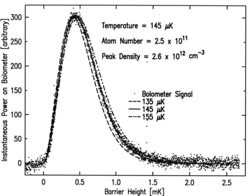
, 300
2- . Temperature = 145 IK
e250 Atom Number = 2.5 x 10¹¹
I-2 - Peak Density - 2.6 x 101 cm E200 -0A
-5\
%
0 150 -\\
Bolometer Signal --- 135pK \ -145 K a100 - -- 55 A 50 0 -0-U) .. . ' - I I I I 0 0.5 1.0 1.5 2.0 2.5 Barrier Height [mK]Figure 2-7: Bolometric determination of the sample temperature. The power de-posited on the bolometer is recorded as a trap confinement barrier is lowered. The power measures the number of atoms with energy equal to the barrier height. The smooth curves are the expected distributions for various sample temperatures. tive bolometer[24, 55]. A robust and reliable method of measuring the temperature[56] and density[51] of the hydrogen sample is to record the recombination energy while lowering the magnetic barrier and releasing the atoms from the trap.
2.5.1
Bolometric Temperature Measurement
If the barrier is lowered slowly compared to the time for atoms to escape, recombine, and deposit energy on the bolometer, the power deposited is proportional to the number of atoms in the sample at the energy of the barrier. Provided the release time is shorter than the collisional rethermalization time, the thermal distribution of atoms in the trap will not change during the dump, and from the bolometric data and a knowledge of the magnetic field, one can find the sample temperature (Fig. 2-7).
Considering the time scale constraints mentioned above and experimental de-tails such as signal to noise of the measurement and inductive time constants of the magnets, the bolometric determination of temperature is only reliable for samples
4.5 . , 4.0 3.5 2 3.0 2.5 2.0 1.5 1.0 0 50 100 150 200 Time [seconds]
Figure 2-8: Decay of a trapped hydrogen sample. The sample density is found from the slope of N(0)/N(t), the inverse of the normalized total number of atoms remaining
in the trap. The data shown indicates a density of 6.0 x 1013 cm-3.
temperatures between 100 pK and 5 mK and densities below 1014 cm-3.
2.5.2
Bolometric Density Measurement
One can measure the sample density by releasing the atoms from the trap after holding them for different times following the forced evaporation. The total recombination energy deposited on the bolometer by a sample held for a time t is proportional to N(t), the number of atoms remaining in the trap at time t. N(t) decreases with time due to dipolar decay and evaporation, as shown in Fig. 2-8.
By integrating the local dipolar decay loss rate (Eq. 2.1) over the trap volume,
one finds
V2(T) 2
Ndip = -g 2(;) N2(t), (2.3)
where Ngdi is the atom loss rate due to dipolar decay, and Vm(T) f d3 , e-mU(r)/kBT
is an effective volume.
While measuring the decay, atoms are also lost due to evaporation. To maintain thermal equilibrium, for every r7 - 2 atoms lost due to dipolar decay, 1 atom must
evaporate[51]. Thus N = Ndip + Nevap - NAdip( - 1)/(7 - 2), and
N(0) 1 = 1 +
(
T - I) V2(T) gno(0)t(24 (2.4)N(t) ( - 2 V1(T)
where no(t) is the peak density in the trap at time t, The value of V2(T)/V1(T)
is found numerically for each trap configuration, but to a good approximation, one can describe the potential by the potential energy density of states exponent, 6:
d'r oc U6-1dU. In a linear quadrupole trap, 6 = 2 and V2(T)/V1(T) . (1/2)6 ~ .25.
For cold samples, which have settled nearer the bottom of the trap, the potential is
harmonic in the radial direction, not linear, and 6 can be significantly different.
From the relative number of atoms measured with the bolometer, and a knowledge of the trap shape, one can extract the initial peak density. The number of atoms in the sample and the absolute sensitivity of the bolometer can then be found from
N(0) = V (T)rno (0).
The slope of the sample decay curve is reproducible to a few percent for identi-cally prepared samples. The dominant uncertainty in this measurement, however, is systematic, arising from imperfect knowledge of our trapping fields. This limits the accuracy of the measurement of no(0) to about 10-20%. Any error in the calculation of g would also be reflected in the inferred densities.
At temperatures below about 100 pK the trapping magnetic fields are so low that additional contributions from magnetic materials and trapped fluxes in the supercon-ducting magnets become significant and the trap is not well known. The bolometric
method for measuring no then becomes unreliable.
Probing the trapped gas with bolometric techniques is limited by the escape time
of the atoms and it also necessitates the destruction of the sample. Spectroscopic
methods offer the possibility of monitoring the gas in situ. The Amsterdam hydrogen trapping group implemented Lyman-alpha 1S-2P spectroscopy of the sample [57], and then, to overcome the limitations imposed by the large natural linewidth of
the 1S-2P transition, they developed resonance enhanced two-photon spectroscopy
is enhanced by tuning one laser frequency near resonance with an intermediate 2P state
[58].
The MIT hydrogen trapping group chose an alternative path and pursued two-photon 1S-2S spectroscopy as a probe of the trapped gas.Chapter 3
Overview of
1S-2S
Spectroscopy in
a Trap
This chapter gives an overview of the 1S-2S spectroscopy component of the experi-ment, as well as a bit of historical perspective. The laser system was designed and built by J. Sandberg and C. Cesar, and more details are available in their Ph.D. theses [59, 60].
High resolution spectroscopy is a useful probe of the trapped hydrogen gas, but the observations reported here also show that the physics of the excitation is of interest
by itself. The two-photon spectrum is novel, and the long coherence time of the
laser-atom interaction makes the atomic motion much more important than it is for normal one-photon transitions. The excitation also probes atom-atom interactions and correlations in ways which are not yet completely understood.
3.1
Background
The two-photon 1S-2S transition was first observed in 1975 in a gas cell[61], and the experimental linewidth was limited to about 100 MHz by the pulsed laser source. Improvements in nonlinear optical frequency generation made CW experiments pos-sible, first in a gas cell at about 0.2 torr [62] where the linewidth was collisionally limited to a few MHz, and then in a liquid nitrogen temperature atomic beam [63]
where the linewidth of 50 kHz was due to the second order Doppler-shift and finite interaction time of the atoms with the laser. By cooling the atomic beam to about
5 K, and selecting the signal from only the coldest atoms, the resolution has reached
about 2 kHz[64].
By comparing the 1S-2S transition frequency to that of another electronic
hy-drogen transition, one can determine the Rydberg constant and Lamb shift [8, 9],
and the deuteron radius can be determined by comparing the 1S-2S frequency in hydrogen and deuterium [8, 65]. The 1S-2S frequency in hydrogen is fis-2s =
2, 466, 061, 413,187.34(84) kHz [9], and this is the most accurately known frequency in the UV or optical region.
In the late 1980's the MIT Ht trapping group, in the quest for BEC, set out to excite the 1S-2S transition in a trapped sample in order to study the gas in situ.
A secondary goal was high resolution spectroscopy of the cold atoms. In a trap the
possible interaction time is long, and at the low thermal velocities, the second order Doppler-shift is negligible.
3.2
Two-Photon Excitation
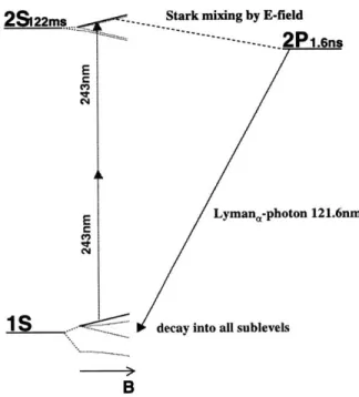
Figure 3-1 shows a sketch of the levels involved in 1S-2S spectroscopy of trapped hydrogen. The angular momentum is zero for both the 1S and 2S states, so the transition cannot be driven by one photon. An atom can absorb two 243 nm photons, however, and be excited to the 2S state through an intermediate virtual P level. For a transition to occur, an atom must absorb two photons in a time less than h/A, where A = (Ep - hv) is the laser detuning from Ep, the energy of the P level. The excitation rate varies as the square of the laser intensity, and for a given intensity, the rate is much lower than for a one photon transition. The 2S state is metastable
(Tis = 122 ms) because an unperturbed 2S atom can only radiatively decay to ground
2 5122ms --... Stark mixing by E-field ---2P1.6ns E C'4 E Lyman,-photon 121.6nm CB
55 decay into all sublevels
B
Figure 3-1: Level scheme for 15-2S spectroscopy of magnetically trapped atomice
hydrogen. Trapped F = 1, mF = 1, 1S atoms are excited to the metastable F =
1, mF = 1, 2S state by absorption of two 243 nm photons. An applied electric
field Stark mixes some 2P character into the excited state wavefunction and causes prompt radiative decay to the ground state through emission of a single Lyman-alpha
photon (121.6 nm). 1S and 2S F = 1, mF = 1 atoms see the same magnetic trapping
potential.
3.3
Detection Scheme
The sample is optically thin to the laser radiation, even on resonance, so it is not feasible to monitor the excitation rate by measuring direct absorption of the laser. However, photoexcitation can be detected by monitoring fluorescence from the excited state. The signal to noise ratio can be greatly enhanced by using a pulsed scheme (Fig.
3-2), in which each excitation pulse is followed by the application of a short electric
field pulse (-- 10 V/cm). This Stark mixes some 2P character into the excited state wave function (See Sec. 4.4.3), and causes 2S atoms to promptly decay to the ground state through emission of a single Lyman-alpha photon (121.6 nm) which can be detected by a microchannel plate (MCP) [67, 68].
f=503.5 mm
fused silica lens
243 electric field w trapped atoms Lyman-alpha p ires hotons R=250 mm BK7 mirror MgF2 window MgF2 Lyman-alpha filter
C5w/
V.-MCP assembly -24 Mn 60 V 1155"VV16 pF - --- - 50 k( ) | 2100 V to amp ler cm 48 cm 46 cm 2 cm o cm -2 cm -24 cm -30 cm -32 cm -34 cmFigure 3-2: Excitation and detection. Trapped atoms are excited to the 2S state
by the 243 nm standing wave laser field which passes on axis. The laser is blocked,
and ±100 V is applied across the electric field wires, producing a 10 V/cm field in the cell. This causes the 2S atoms to rapidly decay through emission of 121.6 nm Lyman-alpha photons. Approximately 10- of these photons are detected with a microchannel plate assembly. The aspect ratio of the figure is 1:1
M r5 0 nm, laser -4 0 00
I I I I
background counter
signal counter applied E field
stray E field counter
laser counter
laser
-500 0 500 1000 1500
Time [pus]
Figure 3-3: Typical timing sequence for 1S-2S excitation and detection.
mechanical chopper modulates the laser beam with 50% duty cycle and 400 Ps pulse length. The electric field pulse is typically 12 ps long, and the resulting signal pulses are recorded by a counter enabled during this time. During this Stark quench the peak count rate can exceed 10 MHz. The number of signal Lyman-alpha counts recorded as a function of laser frequency is the photoexcitation spectrum.
Additional counters during each timing sequence are used for diagnostic purposes. The laser power can vary 10-20% during the recording of one spectrum, and its level is monitored by a counter gated open for 25 ps during the laser pulse. The count rate from scattered laser photons, which can exceed 100 kHz, is proportional to laser power. Following the laser pulse, but before the Stark quench, a counter enabled for 25 pus monitors the Lyman-alpha fluorescence caused by stray electric fields. The count rate can be used to measure the value of the field. Typical stray fields in the cell are on the order of a half volt per centimeter or less, and give the 2S state a lifetime of milliseconds (Sec. 4.4.3). A counter after the quench records dark counts (- 200 Hz) for 25 /is. These counts arise chiefly from long lived fluorescence from
organic materials in the cell which were excited by the laser, and the measured rate can be used to establish the background count rate, which can be subtracted when measuring very weak 1S-2S signals.
This sequence is repeated for typically 10-100 laser pulses for each laser frequency.
3.4
Microchannel Plate Photon Counter
The MCP assembly is shown in Fig. 3-2. The top plate is a 50 mm diameter, 0.6 mm thick lead glass disk with 60% open area in the form of an array of 10 pm diameter channels[68]. Each channel has a length to diameter ratio of 60:1. The top surface is coated with CsI to decrease the work function for efficient production of electrons
by impinging vacuum ultraviolet photons. The top surface is positively biased by 60
volts with respect to the surrounding housing to guide electrons into the channels. Approximately 1000 volts is applied across the channels to accelerate the electrons. Collisions with the channel walls eject more electrons and create an electron shower. Each channel acts as an electron multiplier with a gain of about 104.
The bottom plate is similar in structure to the top, but it has a length to di-ameter ratio of 40:11 for its channels and is uncoated. With 2 plates, the gain is about 106 so that a single photon results in a 1 mV, 5 ns pulse into 50 Q which is capacitively coupled to a high bandwidth video amplifier (x100). Amplified pulses are discriminated and turned into logic pulses which are counted at rates up to 100 MHz. The quantum efficiency of the assembly for 121 nm photons was calibrated against a Hamamatsu R972 photomultiplier tube [69] and found to be 25%. Due to a small solid angle
(~
10- sr), absorption of Lyman-alpha in optical elements, and MCP quantum efficiency, only 10-' of the emitted photons are detected.To be close to the atoms, the MCP is mounted inside the cryostat. At low tem-perature, the replenishment of the charge in a single channel after it fires can take seconds. During the recovery time, that channel is effectively blind to photons. When a significant fraction of the channels fire during one recharging time, the quantum ef-ficiency of the MCP drops. This implies a maximum sustainable counting rate which is about 20 kHz at 20 K, 200 kHz at 80 K, and greater than a MHz at room tem-perature. If precautions were not taken, counts due to scatter from the laser would


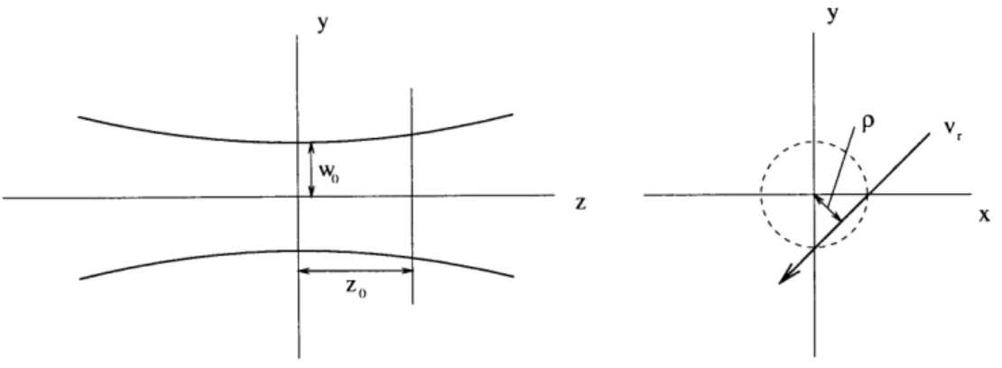
![Figure 4-2, which is taken from [77], shows cross sections of the laser beam and](https://thumb-eu.123doks.com/thumbv2/123doknet/13793598.440641/54.918.138.811.118.604/figure-taken-shows-cross-sections-laser-beam.webp)