Cluster Analysis of Downscaled and Explicitly
Simulated North Atlantic Tropical Cyclone Tracks
The MIT Faculty has made this article openly available.
Please share
how this access benefits you. Your story matters.
Citation
Daloz, Anne S., S. J. Camargo, J. P. Kossin, K. Emanuel, M. Horn,
J. A. Jonas, D. Kim, et al. “Cluster Analysis of Downscaled and
Explicitly Simulated North Atlantic Tropical Cyclone Tracks.” J.
Climate 28, no. 4 (February 2015): 1333–1361. © 2015 American
Meteorological Society
As Published
http://dx.doi.org/10.1175/JCLI-D-13-00646.1
Publisher
American Meteorological Society
Version
Final published version
Citable link
http://hdl.handle.net/1721.1/98015
Terms of Use
Article is made available in accordance with the publisher's
policy and may be subject to US copyright law. Please refer to the
publisher's site for terms of use.
ANNES. DALOZ,aS. J. CAMARGO,bJ. P. KOSSIN,cK. EMANUEL,dM. HORN,eJ. A. JONAS,f D. KIM,bT. LAROW,gY.-K. LIM,hC. M. PATRICOLA,iM. ROBERTS,jE. SCOCCIMARRO,k
D. SHAEVITZ,lP. L. VIDALE,mH. WANG,nM. WEHNER,oANDM. ZHAOp
aSpace Science and Engineering Center, University of Wisconsin–Madison, Madison, Wisconsin bLamont-Doherty Earth Observatory, Columbia University, Palisades, New York
cNOAA/National Climatic Data Center, Asheville, North Carolina dMassachusetts Institute of Technology, Cambridge, Massachusetts eSchool of Earth, University of Melbourne, Melbourne, Victoria, Australia
fCenter for Climate Systems, Columbia University, New York, New York, and Global Modeling and Assimilation
Office, and Goddard Earth Sciences Technology and Research/I.M. Systems Group, NASA Goddard Space Flight Center, Greenbelt, Maryland
gFlorida State University, Tallahassee, Florida
hGlobal Modeling and Assimilation Office, and Goddard Earth Sciences Technology and Research/I.M. Systems
Group, NASA Goddard Space Flight Center, Greenbelt, Maryland
iTexas A&M University, College Station, Texas jMet Office Hadley Centre, Devon, United Kingdom
kIstituto Nazionale di Geofisica e Vulcanologia, Bologna, and Centro Euro-Mediterraneo sui Cambiamenti Climatici, Lecce, Italy lDepartment of Applied Physics and Applied Mathematics, Columbia University, New York, New York
mNational Centre for Atmospheric Science, Department of Meteorology, University of Reading, Reading, United Kingdom nNOAA/NWS/NCEP/Climate Prediction Center, College Park, and Innovim, LLC, Greenbelt, Maryland
oLawrence Berkeley National Laboratory, and University of California, Berkeley, Berkeley, California pNOAA/Geophysical Fluid Dynamics Laboratory, Princeton, New Jersey
(Manuscript received 11 October 2013, in final form 5 November 2014) ABSTRACT
A realistic representation of the North Atlantic tropical cyclone tracks is crucial as it allows, for example, explaining potential changes in U.S. landfalling systems. Here, the authors present a tentative study that examines the ability of recent climate models to represent North Atlantic tropical cyclone tracks. Tracks from two types of climate models are evaluated: explicit tracks are obtained from tropical cyclones simulated in regional or global climate models with moderate to high horizontal resolution (18–0.258), and downscaled tracks are obtained using a downscaling technique with large-scale environmental fields from a subset of these models. For both configurations, tracks are objectively separated into four groups using a cluster technique, leading to a zonal and a meridional separation of the tracks. The meridional separation largely captures the separation between deep tropical and subtropical, hybrid or baroclinic cyclones, while the zonal separation segregates Gulf of Mexico and Cape Verde storms. The properties of the tracks’ seasonality, intensity, and power dissipation index in each cluster are documented for both configurations. The authors’ results show that, except for the seasonality, the downscaled tracks better capture the observed characteristics of the clusters. The authors also use three different idealized scenarios to examine the possible future changes of tropical cyclone tracks under 1) warming sea surface temperature, 2) increasing carbon dioxide, and 3) a combination of the two. The response to each scenario is highly variable depending on the simulation considered. Finally, the authors examine the role of each cluster in these future changes and find no preponderant contribution of any single cluster over the others.
Corresponding author address: Anne Sophie Daloz, Space Science and Engineering Center, University of Wisconsin–Madison, 1225 West Dayton Street, 11th floor, Madison, WI 53704.
E-mail: adaloz@wisc.edu DOI: 10.1175/JCLI-D-13-00646.1
1. Introduction
Tropical cyclones are one of the most devastating phenomena in the world due to their strong winds and heavy precipitation extending over wide areas (e.g., Scoccimarro et al. 2014;Villarini et al. 2014). Thus, there has been a growing demand for better understanding these phenomena and simulations of the response of tropical cyclone activity to climate change. In the past years, many studies have focused on the impact of cli-mate change on tropical cyclone frequency and intensity (e.g.,Gualdi et al. 2008;Knutson et al. 2010;Zhao and Held 2010;Stocker et al. 2014). Recently, a few studies evaluated the impact of climate change on tropical cy-clone tracks over the North Atlantic basin. Murakami and Wang (2010) used a high-resolution global atmo-spheric model (20 km), whileColbert et al. (2013)used a beta advection model with winds from phase 3 of the Coupled Model Intercomparison Project (CMIP3); both studies showed a decrease in straight moving storm tracks reaching the Gulf of Mexico and the Caribbean Sea, as well as an increase in recurving tracks reaching the cen-tral Atlantic. These variations in tropical cyclone trajec-tories are very important as they are a potential cause for changes in the location of landfalling tropical cyclones.
Murakami and Wang (2010)found that these changes in tropical cyclones tracks were caused by an eastward shift in genesis location. On the other hand, Colbert et al. (2013)attributed the projected changes in tropical cyclone trajectories to the large-scale steering flow. Camargo (2013)analyzed the North Atlantic tracks in the phase 5 of the Coupled Model Intercomparison Project (CMIP5) models and obtained no robust changes in future simulations among the models.Mei et al. (2014) analyzed North Atlantic tropical cyclones track density in observations and one of the high-resolution models in this study and found that, on interannual and decadal time scales, a basinwide mode dominates, which is related to the interannual frequency in the basin.Strazzo et al. (2013)used a spatial lattice technique to analyze two of the models in this study and identified regional biases in the North Atlantic tropical cyclone activity. These studies highlighted the importance of accurately simulating the tropical cyclone tracks in addition to the frequency and intensity of tropical cyclones.
To evaluate the ability of modern climate models to represent the North Atlantic tropical cyclone tracks, the characteristics of simulated tracks are explored through the use of a cluster technique (Kossin et al. 2010). The cluster technique applied to observed tracks leads to a meridional and a zonal separation in four groups. The meridional separation largely captures the separation be-tween deep tropical and subtropical, hybrid or baroclinic
cyclones, while the zonal partition tends to segregate Gulf of Mexico from Cape Verde systems.Figure 1shows the separation of the historical tracks, genesis and land-fall points among each of the four clusters for National Hurricane Center North Atlantic Hurricane Database (HURDAT; Jarvinen et al. 1984) for the period 1950– 2013, similarly to what was shown inKossin et al. (2010) for the 1950–2007 storms. In the four clusters, storms in clusters 1 and 2 tend to form farther north than storms from clusters 3 and 4. Storms from clusters 1 and 3 tend to form farther east than storms from clusters 1 and 4 (cf. Fig. 1). Cluster 2 storms form almost exclusively in the Gulf of Mexico and westernmost Caribbean and usually present a northward component in their tracks. Cluster 1 storms form farther east but also tend to have a pro-nounced northward component. Essentially all classic ‘‘Cape Verde’’ tropical cyclones are found in either cluster 3 or 4. Clusters 3 and 4 are both influenced by the African easterly waves coming from the West African continent. Compared to cluster 4 storms, which tend to maintain their primarily westward track until landfall, cluster 3 storms are more often ‘‘recurving.’’ In this study, we first want to verify that the characteristics of the ob-served tropical cyclone tracks [as discussed in Kossin et al. (2010)and shown inFig. 1] are simulated by the climate models.
The climatological properties of North Atlantic tropical cyclone tracks in moderate- to high-resolution atmospheric climate models are documented in this paper and com-pared to the observations. The model simulations analyzed here have been produced for the U.S. Climate Variability and Predictability Research Program (CLIVAR) Hurri-cane Working Group by various modeling centers. An overview of the U.S. CLIVAR Hurricane Working Group objectives and results is given inWalsh et al. (2015). As far as we know, previously, only one other intercomparison project has focused on the study of tropical cyclone activity: the Tropical Cyclone Climate Model Intercomparison Project (TC-MIP; Walsh et al. 2010). However, in that project a different set of simulations was studied.Daloz et al. (2012)showed that in the TC-MIP simulations the majority of climate models have problems representing tropical cyclone activity on the eastern Atlantic because of biases in large-scale fields and/or African easterly wave activity. These issues will also be examined for some models in this study (depending on availability). Here, both explicit and downscaled North Atlantic tropical cyclone tracks are examined.
The explicit tropical cyclone tracks originated from nine climate models (global and regional) with a spatial reso-lution varying from 0.258 to 18. Tracks were obtained using detection and tracking algorithms that find and track storms in the output of these climate models. Typically,
each modeling group developed their own tracking algo-rithm using very similar but different criteria to define and track the model storms. This is clearly a limitation of our analysis; therefore, our results should be considered ten-tative. This issue will be further addressed below. The tracking algorithms have specific criteria for several dy-namic and thermodydy-namic variables leading to the de-tection and tracking of tropical cyclone–like systems
(Walsh 1997;Camargo and Zebiak 2002;Chauvin et al. 2006). The climate models are forced with prescribed cli-matological sea surface temperatures (SSTs): that is, with the same values every year, varying monthly with the sea-sonal cycle for a climatological season. As the models are forced with climatological SSTs, it will not be possible to consider climate variability in our analysis. The modulation of North Atlantic tropical cyclones by El Niño–Southern
FIG. 1. Observed North Atlantic tropical cyclone tracks, genesis locations, and landfall locations during the period 1950–2013 for HURDAT, as separated by the cluster analysis. This figure is similar to what was shown inKossin et al. (2010)for the period 1950–2007.
Oscillation (ENSO) in the same set of models was ana-lyzed inWang et al. (2014)(global climate models) and Patricola et al. (2014)(regional climate model). Here we will evaluate the ability of the different models to correctly simulate the main characteristics of North Atlantic tropical cyclones, such as track types, frequency, intensity, and duration. A description of the global characteristics of the tropical cyclones in the same set of models for the present climate was presented inShaevitz et al. (2015).
Previous studies showed that a realistic simulation of tropical cyclones structure and intensity requires high horizontal- and vertical-resolution models (Rotunno et al. 2009; Rao et al. 2010; Zhang and Wang 2003; Manganello et al. 2012;Strachan et al. 2013;Walsh et al. 2013; Wehner et al. 2015; Zarzycki and Jablonowski 2014). Manganello et al. (2012) obtained realistic in-tensities as well as eyewall structure with a climate model of horizontal resolution of 0.18. However, the horizontal reso-lution of most climate models (.0.258) is too coarse to ad-equately resolve these storms, especially the most intense storms. Low-resolution climate models (;28–38) are able to produce tropical cyclone–like storms, but some of the tropical cyclone characteristics, such as size and intensity, differ from the observed ones (e.g.,Camargo et al. 2005).
To deal with these high-resolution requirements, sev-eral downscaling techniques have been developed. In the second part of this paper, we analyze the results from tropical cyclones obtained with the statistical–dynamical downscaling technique described inEmanuel (2006)and Emanuel et al. (2006). One benefit of this type of down-scaling technique is to generate a very large number of synthetic storm tracks with realistic intensity based on climate model environmental fields. This technique has been successfully applied to various reanalyses (Emanuel 2010) and climate models (Emanuel et al. 2008, 2010; Emanuel 2013) and coupled with storm surge models (Lin et al. 2012). However, this technique also presents some drawbacks such as the absence of statistics of potential initiating disturbances (e.g., African easterly waves). This point will be further discussed in the article. Here we compare the tracks obtained by downscaling the large-scale variables simulated by four of the climate models analyzed in the first part of the study.
Finally, simple future climate projections are examined. The independent and combined effects of an increase in CO2 and a uniform warming of SST are considered.
Previous studies with prescribed SSTs (e.g.,Sugi et al. 2002; Bengtsson et al. 2007) as well as coupled models (Yoshimura and Sugi 2005;Gualdi et al. 2008;Held and Zhao 2011) showed that, at a global scale, there is a projected small decrease in the global tropical cyclone frequency in future climates [see a review inKnutson et al. (2010)].Yoshimura and Sugi (2005)examined the impacts of increased SST and
CO2on tropical cyclone activity separately. The same
ef-fects were examined byHeld and Zhao (2011), who found that both SST warming and CO2 doubling have an
im-portant role in the global decrease of TC frequency in future climates. In this study, we would like to determine if the results fromHeld and Zhao (2011)are robust across the tropical cyclones from various climate models in the North Atlantic basin, as well as for the tropical cyclones obtained by downscaling these climate models.
Kossin et al. (2010)determined that clusters could contribute differently to the observed trends in the North Atlantic storm frequency in the current climate. They showed that trends are governed by the deep tropical storms (cluster 3), which account for most of the major tropical cyclones. This cluster is therefore very important as it contains some of the most dan-gerous tropical cyclones. Furthermore, several studies showed an intensification of tropical activity in future climates (Chauvin et al. 2006; Oouchi et al. 2006; Knutson et al. 2010;Villarini and Vecchi 2013). One can wonder if the potential intensification of North Atlantic tropical cyclones in the future climate could be attributed to changes in frequency or intensity of a specific cluster. This topic will be explored in the last part of our results.
In summary, the objectives of this study are (i) to ex-amine simulated North Atlantic tropical cyclone tracks from explicit and downscaled simulations and determine if they are able to reproduce the main characteristics of the observed North Atlantic tropical cyclone clusters obtained in Kossin et al. (2010); (ii) to investigate the tropical cyclone track clusters for different models, con-sidering different ways of generating the tropical cyclones (explicitly or downscaling) and different scenarios (cli-matological SST, SST warming, an increase of CO2, or
both); and (iii) to determine if the projected changes in tropical cyclone activity over the North Atlantic basin could be attributed to specific clusters.
Section 2summarizes the cluster technique and de-scribes the models and the tracking algorithms used. In section 3, the characteristics of the explicitly simulated North Atlantic tropical cyclone clusters are analyzed. In section 4, the same analysis is performed for the down-scaled tropical cyclones. Section 5explores, using clus-ters, future changes in frequency and intensity of North Atlantic tropical cyclones. Finally, a summary and a dis-cussion of our results are presented insection 6. 2. Clustering method and data
a. Clustering method
The cluster technique used in this study relies on a mixture of quadratic regression models, which are used
to fit the geographical shape of tropical cyclone tracks. Each component of the mixture model uses a poly-nomial regression curve of storm position against time. Each track is assigned to one of K different re-gression models. Each model is described by a set of different parameters, a regression coefficient, and a noise matrix. The cluster technique is described in detail inGaffney et al. (2007). The technique has al-ready been applied to observed tropical cyclone tracks in various regions, namely the North Atlantic (Kossin et al. 2010), western North Pacific (Camargo et al. 2007), eastern North Pacific (Camargo et al. 2008), Southern Hemisphere (Ramsay et al. 2012), and Fiji (Chand and Walsh 2009).
Kossin et al. (2010) showed that, for North Atlantic observed tropical cyclone tracks, the optimal number of clusters was four. In that study, an in-sample log-likelihood value narrowed down the ideal number of cluster to values between three and six clusters. The final se-lection, four clusters, was qualitatively based on physical characteristics of the basin. The first factor considered was the modulation of the North Atlantic tropical cy-clone activity by the Atlantic meridional mode (AMM) and ENSO. Another selection factor was based on how well the clusters represented subsamples of storm tracks based on geographic location of tropical cyclogenesis. At least four clusters were necessary to correctly characterize the track types that appeared in the sub-samples examined. Based on these combined factors, four clusters was the optimal choice. In this study, we also choose to use four clusters, as we wanted to com-pare the results of the models with those from obser-vations.Figure 1shows the resulting tracks, genesis and landfall locations obtained when applying this cluster technique to the observed North Atlantic tropical cy-clone tracks [extending the results of Kossin et al. (2010)through 2013].
Also the analyses on the observed clusters are per-formed over the period from 1950 to 2013 for the ob-servations.Landsea et al. (2010)showed that including the presatellite era tends to introduce an underestimate of the number of shorter tracks. In our case, including the presatellite era does modify the number of storms in clusters 3 and 4 but does not change the other charac-teristics of the clusters. The results of cluster analysis could be potentially sensitive to the track length; how-ever,Camargo et al. (2007)showed that cluster assign-ments are modified because of the track length only when very drastic changes are done.
b. Explicit simulations
Two types of experiments are used in this study, namely explicit and downscaled simulations, as explained in the Introduction and shown in Fig. 2. The explicit tropical cyclones were generated from nine climate models listed inTable 1. The model simulations were forced with prescribed climatological SST and sea ice from the Hadley Centre Sea Ice and Sea Surface Temperature Experiment dataset (HadISST; Rayner et al. 2003). The radiative gas forcing follows the 1992 Intergovernmental Panel on Climate Change (IPCC) specifications. Four types of simulations are used: a con-trol experiment and three idealized warming scenarios. The control experiment (CTL) is forced with clima-tological SST (climaclima-tological mean of the period 1981–2005). There are three idealized future simulations. The first future experiment corresponds to the climato-logical SST with 2 K added globally, ‘‘plus 2K’’ (p2K). The second future experiment, named ‘‘double CO2’’
(2CO2), is forced with the same climatological SST, but the CO2concentration is doubled in the atmosphere. In
the third future experiment, ‘‘plus 2K and double CO2’’
(p2K2CO2) is the combination of the last two scenarios: that is, the models are forced with climatological SST
with 2 K added globally and a doubling of the CO2
concentration.
c. Tracking algorithms
The simulated tropical cyclones were tracked by each modeling group using the tracking methodology nor-mally adopted by them. The tracking routines used in most groups are based in very similar principles, but there are differences among them. The criteria chosen and the thresholds vary depending on the tracking al-gorithm and the spatial resolution for each model. The
tracking algorithms employed in this study are all de-scribed in theappendix.
Previous studies showed that the frequency of tropical cyclones could be sensitive to the method of identifica-tion of the storms (Walsh et al. 2007;Horn et al. 2014). Horn et al. (2014) showed that the basic differences between tracking schemes are not of primary importance however differences in duration, wind speed, or formation-latitude thresholds are crucial. After homogenization of these thresholds, there is large agreement between differ-ent tracking schemes. The sensitivity of the cluster analysis
TABLE1. Presentation of the explicit and downscaled simulations from CLIVAR. The models are classified going from higher to lower horizontal resolution. (Model name expansions are provided in a searchable list athttp://www.ametsoc.org/PubsAcronymList, under the heading ‘‘Climatic, meteorological, oceanographic, and other models’’.)
Model: institution Horizontal and vertical resolutions; No. of years Type of simulations Name of the simulations in the article Model description reference Reference for the tracking methodology CAM5.1: National Center
for Atmospheric Research (NCAR), United States
0.258, 30 levels; 65 yr Explicit CAM5_E Wehner et al. 2015 Knutson et al. 2007
Downscaled CAM5_D Emanuel et al. 2008 —
WRF: Texas A&M University, United States
0.258, 28 levels; 40 yr Explicit–lateral boundary conditions: NCEP-2
WRF_E Skamarock et al. 2008 Walsh 1997
HIRAM2.1: Geophysical Fluid Dynamics Laboratory (GFDL), United States
0.58, 32 levels; 80 yr Explicit GFDL_E Anderson et al. 2004; Zhao et al. 2009
Zhao et al. 2009
Downscaled GFDL_D Emanuel et al. 2008 — GEOS5: National
Aeronautics and Space Administration (NASA) Global Modeling and Assimilation Office, United States
0.58, 72 levels; 76 yr Explicit GSFC_E Rienecker et al. 2008 Vitart et al. 2003
HadGEM3A: Met Office Hadley Centre, United Kingdom
0.68, 85 levels; 24 yr Explicit HG3A_E Walters et al. 2011 Strachan et al. 2013
ECHAM5: Centro Euro-Mediterraneo per I Cambiamenti Climatici (CMCC), Istituto Nazionale di Geofisica e Vulcanologia (INGV), Italy
0.98, 31 levels; 80 yr Explicit CMCC_E Roeckner et al. 2003; Scoccimarro et al. 2011
Walsh 1997
Downscaled CMCC_D Emanuel et al. 2008 —
GISS-GCM: NASA GISS and Columbia
University, United States
18, 40 levels; 40 yr Explicit GISS_E Schmidt et al. 2014 Camargo and Zebiak 2002
Downscaled GISS_D Emanuel et al. 2008 — GFS: National Centers for
Environmental Prediction (NCEP), United States
18, 64 levels; 40 yr Explicit GFS_E Saha et al. 2014 Zhao et al. 2009
FSU-GCM: Center for Ocean–Atmospheric Prediction Studies (COAPS), Florida State University, United States
18, 27 levels; 15 yr Explicit FSU_E Cocke and LaRow 2000; LaRow et al. 2008
to the tracking techniques (described in theappendix) has been examined for two models using the data from Horn et al. (2014): only the results for the CMCC_E model (cf.Table 1) are presented here. This has to be considered as a tentative analysis, as we could not test all the models and tracking algorithms. Three different tracking algorithms were employed to detect the North Atlantic tropical cyclones tracks. The first tracking al-gorithm is the one originally used by the group for tracking the tropical cyclones; it follows the criteria defined inWalsh (1997). The second one is a modified Commonwealth Scientific and Industrial Research Or-ganization (CSIRO) tracking scheme (Walsh et al. 2007; Horn et al. 2013). Finally, the third algorithm is the one fromZhao et al. (2009). The first and second tracking algorithms have similarities as they both are based on the algorithm ofWalsh (1997); this should be kept in mind as we examine the results of the test.
Figure 3presents the results of the test and shows the location of the genesis points for the four clusters using the three tracking algorithms. Here, our focus is not on the ability of CMCC_E to simulate the clusters, but to evaluate the differences among the clusters using dif-ferent detection schemes.Figure 3shows that the posi-tion of the genesis points in each cluster is very similar when using the tracking algorithms fromWalsh (1997) (Fig. 3a) orHorn et al. (2013)(Fig. 3b). This is certainly due to the similarities in these two tracking algorithms, as explained above. Cluster 1 storms are developing over high latitudes, cluster 2 storms tend to appear over the Gulf of Mexico, and cluster 4 storms appear over the Caribbean Sea. Finally, cluster 3 storms develop over a band going from the Caribbean Islands to the West African coast. Some differences appear when using the tracking scheme fromZhao et al. (2009)(Fig. 3c). Clus-ters 2 and 4 are similar for the three tracking schemes, but some differences appear for clusters 1 and 3. The genesis points of cluster 1 are located farther north, while more
genesis points appear off the West African coast for cluster 3 storms when detected with the scheme from Zhao et al. (2009). However, these differences do not change the general characteristics of the storms in each cluster. For instance, cluster 1 storms, in all three tracking algorithms, are tropical cyclones that tend to develop over higher latitudes, while cluster 3 storms are systems that tend to develop in the eastern part of the Atlantic basin.
Complementary toFig. 3,Table 2presents the num-ber of tropical cyclones detected per year for CMCC_E using the three different tracking algorithms. The num-ber of tropical cyclones detected is the same when using the scheme from Walsh (1997)or the modified CSIRO scheme. However, when using the scheme from Zhao et al. (2009), there are differences. The total number of tropical cyclones per year increases from 1.5 to 2.4, but it does not change the main result: that is, CMCC_E highly underestimates the number of tropical cyclones over the North Atlantic basin. The differences in the number of TC mainly come from clusters 1 and 4, which double with the Zhao scheme.
In summary, while we do not think that using different tracking algorithms for comparing tropical cyclone
FIG. 3. North Atlantic tropical cyclone genesis locations of the tracks for CMCC_E, as separated by the cluster analysis. Tropical cyclones tracks are detected with the tracking algorithm from (a)Walsh (1997), (b)Camargo and Zebiak (2002), and (c)Zhao et al. (2009). Cluster 1 is in dark blue, cluster 2 is in light blue, cluster 3 is in pink, and cluster 4 is in red.
TABLE2. Number of tropical cyclones per year detected with the tracking algorithms from (i)Walsh (1997), (ii)Horn et al. (2013), and (iii)Zhao et al. (2009)for each cluster and the total, for the explicit simulation CMCC_E, and (iv) for the observations (HURDAT: 1950–2013).
CMCC_E Cluster 1 Cluster 2 Cluster 3 Cluster 4 Total
Walsh (1997) 0.3 0.5 0.2 0.5 1.5 Horn et al. (2013) 0.3 0.5 0.2 0.5 1.5 Zhao et al. (2009) 0.8 0.6 0.2 0.8 2.4 Observations 3.5 2.9 3.7 2.3 12.4
tracks is ideal, for the present study, the use of the same tracking algorithm for all the models was not possible. Therefore, we decided to use the tracks available to us, keeping in mind that differences that we find among the models can be due to the differences between the models themselves but also probably be partly attributed to the differences in tracking algorithms. Therefore, we will not specifically compare the number of tropical cyclones between each cluster for the explicit simulations but just discuss cases in which a model highly underestimates or overestimates the number of systems produced compared to the observations and other models. The use of different tracking algorithms modifies some of the characteristics of the clusters (e.g., number); however, it cannot change the ability of a model to produce tropical cyclones. The high underestimation of the number of storms of CMCC_E cannot be completely removed by a change in tracking algorithm. The difference of algorithm only slightly changes the total number of storms, especially the num-ber of weak storms, which can be more sensitive to the specific thresholds in the different tracking algorithms. So, the comparison of some of the characteristics of the clusters between observations and different models is still pertinent.
d. Downscaled simulations
For the downscaled simulations, the technique de-veloped byEmanuel et al. (2006)was used. The down-scaled simulations are described inFig. 2andTable 1. The downscaling technique of Emanuel et al. (2006, 2008) consists of, first, initiating storms by random seeding in space and time with warm-core vortices that have peak wind speeds of 12 m s21. The random ‘‘seeds’’ are planted everywhere and at all times, regardless of latitude, sea surface temperatures, season, or other factors, except that storms are not allowed to form equatorward of 28 latitude. Then the storms are propa-gated forward with a beta and advection model driven by winds derived by the four climate models presented inTable 1. The seeds are not considered to form tropical cyclones unless they develop winds of at least 21 m s21. Only four downscaled simulations were performed be-cause of a lack of data from the climate models output when the downscaled simulations were performed.
To derive the storm intensity along each track, a very high-resolution coupled atmosphere–ocean hurricane model is used: namely, the Coupled Hurricane Intensity Prediction System (CHIPS; Emanuel et al. 2006). CHIPS is an axisymmetric atmospheric model in po-tential radius coordinates (Schubert and Hack 1983). CHIPS is coupled to a simple, one-dimensional ocean model that captures most of the effects of upper-ocean mixing. The atmospheric model can reach a couple of
kilometers of horizontal resolution. The potential radius coordinates permit obtaining high resolution for the eye and the eyewall using a relatively small number of radial nodes. Inputs to CHIPS are in the form of monthly-mean climatological potential intensity (which combines the thermodynamic control on tropical cyclone intensity of both the sea surface temperature and the environ-mental atmospheric temperature profile). Ocean mixed layer depth and thermal stratification of the ocean be-low the mixed layer are all interpolated to the position and time of the storm.Emanuel et al. (2004)studied the effect of using monthly-mean climatological intensity instead of daily data and found that it was minimal in most cases.
Previous studies have already demonstrated that the tropical cyclone activity from this downscaling tech-nique is generally realistic (e.g., Emanuel et al. 2006; Emanuel 2010). For instance, Emanuel et al. (2006) showed that, when driven by NCAR–NCEP reanalysis (Kalnay et al. 1996), the synthetic tracks obtained cap-ture correctly the observed spatial and seasonal vari-ability of tropical cyclones around the globe. However, this technique presents some drawbacks such as the lack of the feedbacks between the tropical cyclones and their environment. Also, notably absent from this technique is the statistics of potential initiating disturbances, such as African easterly waves. This may impact the realism of the timing of the development of tropical cyclones over the eastern part of the North Atlantic basin. 3. Climatology of clusters from explicit simulations a. Tracks and genesis
Figure 4 presents the general climatology of North Atlantic tropical cyclone genesis by cluster membership for observations (Fig. 4a: HURDAT dataset period 1950–2013; Jarvinen et al. 1984) and the nine explicit simulations (Figs. 4b–j) described in Table 1. Table 3 summarizes various measures of tropical cyclone activity for each of the four clusters shown inFig. 4for observa-tions and the nine models. These figures and Table 3 clearly show the separation of the North Atlantic tropical cyclone genesis (Fig. 4) locations in each of the four clusters, with meridional and zonal separations between the clusters. The separation between the clusters is ex-amined deriving the mean position of TCs in each cluster (cf.Table 3). The number of North Atlantic tropical cy-clones for most of the explicit simulations is smaller than in observations. For some models, there were only 10 or 15 tropical cyclones over the entire time period of the control simulation. To have a large sample size and to apply the same procedure for all the simulations, the cluster analysis was performed for each model using all
the ensembles and scenarios simultaneously. We did sensitivity tests for the model with most storms (GFDL_E) and determined that applying the cluster analysis to all the scenarios simultaneously would not lead to different results than if we applied the cluster analysis for each scenario separately (not shown). It is important to notice that the cluster analysis has no knowledge of which sim-ulation the track belongs to. Therefore, as we wanted to use the same methodology for all models, the models with a very low number of storms restricted us to apply the
cluster analysis to all the tracks in a model together, in-dependently of the scenario. Once the storms are classi-fied in clusters, we examine if there are differences in the characteristics of the clusters for the different scenarios.
The comparison of the cluster analysis applied to North Atlantic tropical cyclones in observations (Fig. 4a) with the simulated tropical cyclones in GFDL_E (Fig. 4d) shows encouraging results. There is a good agreement in terms of cluster separation (Table 3) for the genesis lo-cations (Fig. 4) between the observations and GFDL_E.
FIG. 4. North Atlantic tropical genesis locations of the tracks for observations and explicit simulations, as separated by the cluster analysis. Cluster 1 is in dark blue, cluster 2 is in light blue, cluster 3 is in pink, and cluster 4 is in red. The models are presented following the alphabetical order with first the four models that were used for both explicit and downscaled simulations and then the five other explicit simulations.
The left panels of Fig. 5 show the tracks in each four clusters for GFDL_E. Compared to observations in Fig. 1, GFDL_E shows a good representation of the tracks (Figs. 5a,c,e,g) and landfall (not shown) locations. Figures 4a and 4d show that, for both the observations
and this explicit simulation in clusters 1 and 2, tropical cyclones tend to form farther north than in clusters 3 and 4, while the tropical cyclones in clusters 1 and 3 tend to form farther east than in clusters 2 and 4. In cluster 2, tropical cyclones tend to form almost exclusively in the
TABLE3. Comparison of various measures by cluster for the observations from HURDAT (1950–2013) and the nine explicit simu-lations. Percent values (in parentheses) represent the proportions of tropical cyclones from each cluster to the total number of tropical cyclones.
All runs Dataset Cluster 1 Cluster 2 Cluster 3 Cluster 4 Total No. of TC per year OBS 3.5 (28%) 2.9 (24%) 3.7 (30%) 2.3 (18%) 12.4
CAM5_E 2.6 (26%) 3.5 (35%) 1.7 (18%) 2.1 (21%) 9.9 CMCC_E 0.3 (18%) 0.5 (33%) 0.2 (14%) 0.5 (35%) 1.5 GFDL_E 3.7 (34%) 2.2 (21%) 2.8 (26%) 2.0 (19%) 12.7 GISS_E 1.7 (28%) 1.7 (28%) 1.7 (29%) 0.9 (15%) 6.0 FSU_E 5.5 (22%) 6.4 (24%) 6.4 (24%) 7.9 (30%) 26.2 GFS_E 1.7 (19%) 2.1 (25%) 3.6 (42%) 1.1 (14%) 8.5 GSFC_E 1.0 (17%) 1.5 (26%) 1.6 (29%) 1.6 (28%) 5.7 HG3A_E 2.1 (25%) 2.3 (27%) 2.2 (26%) 1.9 (22%) 8.5 WRF_E 1.2 (5%) 6.5 (29%) 6.2 (27%) 8.7 (39%) 22.6 Mean position (latitude, longitude) OBS 278N, 648W 228N, 848W 148N, 378W 148N, 658W
CAM5_E 248N, 598W 178N, 728W 128N, 188W 158N, 308W CMCC_E 298N, 668W 218N, 868W 188N, 508W 158N, 808W GFDL_E 288N, 518W 238N, 768W 148N, 298W 158N, 588W GISS_E 328N, 698W 188N, 808W 348N, 448W 158N, 558W FSU_E 188N, 668W 98N, 448W 118N, 408W 108N, 498W GFS_E 258N, 488W 228N, 668W 148N, 318W 288N, 328W GSFC_E 238N, 538W 178N, 768W 78N, 298W 78N, 408W HG3A_E 118N, 788W 128N, 848W 168N, 438W 168N, 788W WRF_E 188N, 208E 248N, 648W 148N, 188W 178N, 788W Mean duration per TC (days) OBS 6.2 5.6 10.6 8.4
CAM5_E 8.1 8.5 12.6 13.1 CMCC_E 2.1 3.3 4.0 3.6 GFDL_E 8.3 9.1 10.1 9.8 GISS_E 15.6 14.3 14.6 13.7 FSU_E 10.6 15.1 11.4 12.3 GFS_E 5.1 5.4 5.5 5.4 GSFC_E 3.6 3.3 3.8 3.5 HG3A_E 16.2 16.6 15.6 11.4 WRF_E 4.8 4.3 6.8 5.0 Mean LMI per TC (m s21) OBS 34 34 43 44
CAM5_E 46 48 42 58 CMCC_E 21 22 23 22 GFDL_E 44 45 42 43 GISS_E 16 14 17 12 FSU_E 34 37 35 38 GFS_E 22 21 22 24 GSFC_E 20 17 16 16 HG3A_E 23 26 32 26 WRF_E 29 37 34 39
Mean PDI per TC (1010m3s22) OBS 1.2 1.0 4.0 2.8
CAM5_E 3.5 3.6 4.9 8.8 CMCC_E 0.1 0.2 0.3 0.2 GFDL_E 3.3 3.5 4.6 3.9 GISS_E 0.2 0.1 0.2 0.1 FSU_E 1.4 2.5 1.6 2.3 GFS_E 0.2 0.3 0.4 0.3 GSFC_E 0.1 0.1 0.1 0.1 HG3A_E 0.4 0.8 1.4 0.6 WRF_E 0.9 1.2 1.8 1.8
FIG. 5. North Atlantic tropical cyclone tracks for (left) GFDL_E and (right) GFDL_D, as separated by cluster analysis.
Gulf of Mexico and westernmost Caribbean, while in cluster 1 they tend to form farther east. Clusters 1 and 2 present a pronounced northward component in their tracks (Figs. 1and5). Essentially all classic ‘‘Cape Verde tropical cyclones’’ are found in clusters 3 and 4. Cluster 4 tropical cyclones tend to maintain their primarily west-ward track until landfall (straight movers;Figs. 1and5). Cluster 3 storms are more likely to ‘‘recurve’’ (Figs. 1and 5), which characterizes the evolution of a storm track from westward and northward to eastward and northward (e.g.,Hodanish and Gray 1993). More details about the observed clusters characteristics can be found in Kossin et al. (2010).
Unfortunately, the other models present substantial differences in their position of tropical cyclone genesis (Figs. 4b–jandTable 3) when compared to the obser-vations (Fig. 4a). As an example, the left panels ofFig. 6 present the resulting tracks for the four clusters of GISS_E. The large disparity in the representation of tropical cyclone activity among the models can be due to several reasons, such as differences in physical param-eterizations, especially convection schemes (e.g., Kim et al. 2012;Zhao et al. 2012), vertical or horizontal res-olutions (Rotunno et al. 2009;Rao et al. 2010;Zhang and Wang 2003;Manganello et al. 2012;Walsh et al. 2013), and dynamical cores (Reed and Jablonowski 2011a,b,2012). Half of the models examined here have a horizontal resolution around 18 (HG3A_E, CMCC_E, GISS_E, GFS_E, and FSU_E); however, as an accurate simulation of tropical cyclones requires high-resolution models (e.g., Rotunno et al. 2009; Manganello et al. 2012;Walsh et al. 2013), 18 is still too coarse to represent adequately many characteristics of tropical cyclones, es-pecially intensity. However, the spatial resolution is not the only explanation for the model biases. WRF_E has the highest resolution among the models, but in WRF_E cluster 1 the tropical cyclones have an unrealistic genesis location (Fig. 4j) over the West African continent. In this case, this bias is probably coming from the tracking al-gorithm, which starts tracking the storms while they are still easterly waves over the West African continent.
Daloz et al. (2012)showed that many climate models present large biases when simulating tropical cyclone activity over the eastern Atlantic (clusters 3 and 4 storms). They mainly attributed these model biases to differences in large-scale fields and/or difficulties in sim-ulating the African easterly waves over the West African coast. To further explore this hypothesis,Table 4presents the mean African easterly wave activity over the West African continent for a subset of explicit simulations and the reanalysis ERA-Interim (1979–98; Dee et al. 2011). The African easterly wave activity was obtained using the technique fromFyfe (1999). A maximum of variance of
the 2–6-day filtered meridional wind at 850 hPa over western Africa is defined as a maximum in African easterly waves activity.
Table 4 also present the mean vertical wind shear defined as the 24-h averaged vector difference between 200 and 850 hPa over the east Atlantic basin for the same subset of explicit simulations. High values of vertical wind shear are known to be an unfavorable environment for the formation of tropical cyclones (Gray 1968). Values of vertical wind shear over around 10 m s21are detrimental to tropical cyclone development. Unfor-tunately, these variables could not be calculated for all the models, as the necessary data were not available. GISS_E (Fig. 4e) generates very few or misplaces cluster 3 tropical cyclones. The genesis locations for their cluster 3 cyclones are in the center of the North Atlantic basin around 408N, while in observations genesis occurs near the West African coast around 208N. In agreement with Daloz et al. (2012), GISS_E highly underestimates Afri-can easterly wave activity compared to ERA-Interim (cf. Table 4). On the other hand, CMCC_E (Fig. 4c) presents a reasonable African easterly wave activity but does not develop many tropical cyclones in the eastern Atlantic. Also,Bain et al. (2014)showed that the Met Office model (HG3A_E) is able to represent African easterly wave features at the climate time scale; however, it under-estimates the strength and the frequency of the wave. This could partly explain the low tropical cyclone activity on the eastern part of the Atlantic basin (Fig. 4i). The unfavorable values of vertical wind shear (cf. Table 4) help explain why the genesis is concentrated in the western part of the Atlantic. It also interesting to note that, for GFS_E (Fig. 4g), most of the tropical cyclone genesis is located in the eastern part of the Atlantic basin. Furthermore, this model presents a very high-level Af-rican easterly wave activity, nearly triple what is observed in ERA-Interim, which could be associated with low values of vertical wind shear. Humidity fields would also have been a good indicator for explaining some of the differences among the models, but they were not avail-able at the same pressure level for all the models. b. Storm characteristics
In observations (HURDAT), the annual-mean num-ber of North Atlantic tropical cyclones is 12.4 (tropical storms and hurricanes: i.e., named storms) for the period 1950–2013 while in the models’ explicit simulations this number varies from 26.2 and 22.6 tropical cyclones per year in the FSU_E and WRF_E models, respectively, to 1.5 tropical cyclones per year for the CMCC_E model. CAM5_E, HG3A_E, GFDL_E, and GFS_E have the most realistic values, with approximately 10 tropical cyclones per year, while GSFC_E and GISS_E have
only around 6 tropical cyclones per year. In observa-tions, more than half of the tropical cyclones (52%) are members of clusters 1 and 2, which form over higher latitudes (north of 208N) and will be called here the northernmost tropical cyclones. In contrast, tropical cy-clones in clusters 3 and 4 typically have genesis locations in the deep tropics (south of 208N) and will be called here the southernmost tropical cyclones. As explained in sec-tion 2, the number of tropical cyclones per year inTable 3 is only indicative and will not be discussed because of the differences in tracking methodology. Just for confirming the difficulty of analyzing this value, for most of the ex-plicit models, the standard deviation for the mean num-ber of tropical cyclones per year was high, showing a large variation around the mean.
In observations (cf.Table 3), the northernmost trop-ical cyclones have a mean lifetime of 6.2 and 5.6 days, while the southernmost tropical cyclones mean lifetimes are longer with 10.6 and 8.4 days as they have more time to travel over the Atlantic Ocean before touching the coasts. Tropical cyclones for most of the explicit simu-lations have very similar mean lifetime duration for all clusters. Also, the simulated mean duration of tropical cyclones is usually different from the observations, with the northernmost tropical cyclone lifetime varying from 2.1 days for CMCC_E to 16.6 days for HG3A_E. In the case of the southernmost tropical cyclones, the mean lifetime varies from 3.5 days for GSFC_E to 15.6 days for HG3A_E. The comparison of mean duration per tropical cyclone is complicated by the fact that the models do not share the same tracking algorithms and the storm duration is highly dependent on the tracking algorithm thresholds. To examine the sensitivity of the storm lifetime to the tracking thresholds, we applied a wind criterion, which depends on the spatial resolution of the model, followingWalsh et al. (2007). For seven of the nine models, our results for lifetime remain basically the same. Therefore, the lifetimes per tropical cyclone are comparable among most models, with exception of GISS_E and GSFC_E, which did not meet the criteria
because of the weak wind speeds of their storms (cf. Table 3).
Table 3also presents a crucial variable for studying tropical cyclones, the lifetime maximum intensity. In observations, the lifetime maximum intensity (LMI; Elsner et al. 2008) has bimodal characteristics. For de-riving the LMI, we used the 10-m wind speed or surface wind speed depending on the availability of the data.1 The bimodal distribution arises from differences in LMI and lifetime duration between the northernmost and southernmost tropical cyclones. The southernmost trop-ical cyclones tend to reach higher intensities, because they stay longer over warm tropical waters with clima-tologically low vertical wind shear (Kossin et al. 2010). The first peak in LMI appears for the northernmost tropical cyclones, which achieve an average of 34 m s21 associated with shorter tracks and colder SSTs. The sec-ond peak appears for the southernmost tropical cyclones, which reach a higher LMI with a mean intensity of 44 m s21, associated with longer tracks and warmer SSTs. The explicit tropical cyclone simulations do not simulate the bimodality of LMI of the northernmost and south-ernmost tropical cyclones, the mean LMI is nearly the same for all clusters and all the simulations. Furthermore, the intensity of the tropical cyclones is underestimated by most the models (CMCC_E, GISS_E, FSU_E, GFS_E, GSFC_E, HG3A, and WRF_E). This is a common bias of climate models (e.g., Yoshimura et al. 2006; Knutson et al. 2007;LaRow et al. 2008;Walsh et al. 2013), because of low model horizontal resolution and convective pa-rameterization. Even WRF_E (Table 3), with the highest resolution (around 0.258), has a mean LMI weaker than the observed LMI despite realistic peak intensities. The two other models (CAM5_E and GFDL_E) tend to overestimate the LMI, which could be due to their higher horizontal resolution.
The destruction that tropical cyclones can potentially cause can be estimated with a power dissipation index (PDI; Emanuel 2005). This index combines the fre-quency, duration, and intensity of the tropical cyclones. The PDI is defined as the integral of the cube of the maximum wind speed of the tropical cyclone over the period considered.Table 3presents the mean PDI per tropical cyclone for each cluster. In the observations, the mean PDI per tropical cyclone is higher for the south-ernmost tropical cyclones with 4.0 3 1010m3s22 for cluster 3 and 2.83 1010m3s22 for cluster 4, while for clusters 1 and 2 it is approximately 1.0 3 1010m3s22. Cluster 3 has the highest PDI per tropical cyclone,
TABLE4. African easterly wave activity averaged over the West African continent (108–208N, 158W–08) and vertical wind shear averaged over the east Atlantic basin (108–208N, 58–158W) for a subset of explicit simulations and ERA-Interim only for the African easterly wave activity. The calculations were realized over the time period of each CTL runs.
Models African easterly wave activity (m2s22) Vertical wind shear (m s21) CMCC 7.7 12.0 GFS 19.7 7.9 GISS 0.4 11.5 ERA-Interim 7.3
1Each center has its own technique for deriving these quantities,
3 1010m3s22for FSU_E (Table 3), because of the low
intensity of these model tropical cyclones. For the other models (CAM5_E and GFDL_E), the mean PDI is overestimated compared to the observed values and goes from 3.33 1010m3s22for GFDL_E to 8.83 1010m3s22 for CAM5_E because of an overestimate both in intensity and mean duration of the simulated tropical cyclones. c. Seasonality
The seasonality of cluster membership is presented in Fig. 7for the observations and the explicit simulations. For observations (Fig. 7a), tropical cyclones of clusters 1 and 2 are prevalent during the early part of the North Atlantic tropical cyclone season (May–July). During this period, the environmental conditions are more fa-vorable for their formation. During this period, ther-modynamic conditions are usually not favorable in the tropics but higher-latitude conditions are good for baro-clinic initiation of storms (McTaggart-Cowan et al. 2008). For cluster 2 storms, the scenario is different: midlatitude frontal systems can often deviate southward into the Gulf of Mexico and provide the baroclinic conditions that are favorable for cyclogenesis (Bracken and Bosart 2000). Cluster 3 tropical cyclones are mainly observed during the peak hurricane season (August– September), because of their strong modulation by Af-rican easterly waves (Landsea 1993), which peak at the same time of the seasonal cycle. During the late season (October–December), tropical cyclones from cluster 1 are predominant, because during those months envi-ronmental conditions are more favorable for the de-velopment of higher-latitude tropical cyclones. Cluster 4 storms present a broader seasonal cycle distribution with no peak in contribution along the season.
Error bars inFig. 7provide an indication of the dif-ferences between the simulations. The large error bars indicate that the models are presenting very different results from the observations and among them. Only three models have tropical cyclones with a similar sea-sonality as in observations, GFDL_E (Fig. 7d), GISS_E (Fig. 7e), and HG3A_E (Fig. 7i). For these models, the early and late seasons are well simulated with the pre-dominance of clusters 1 and 2. However, in midseason
clusters 1 and 2. For some models, this is due to a bias in the proportion of tropical cyclones in a cluster. For ex-ample, WRF_E (Fig. 7j) largely underestimates the number of cluster 1 tropical cyclones, so it cannot simu-late correctly the preponderance of this cluster in the early and late seasons. This is due to a criterion in the tracking algorithm: they do not take into account the storms developing over 308N. GFS_E (Fig. 7g) overestimates the proportion of cluster 3 tropical cy-clones, which leads to an unrealistic preponderance of cluster 3 tropical cyclones in the whole season. The bias in early and late seasons could also come from a misre-presentation of the seasonality of large-scale variables. The seasonality of clusters 1 and 2 is very much influenced by the environmental conditions, as mentioned above. Therefore, favorable conditions for cyclogenesis of the northernmost tropical cyclones might not be happen-ing at the same time in observations and simulations. Furthermore, the large error bars inFig. 7put in evidence the difficulties of the explicit simulations to represent the seasonal cycle of cluster memberships, indicating the large spread among the models.
This section shows that the North Atlantic tropical cy-clones in the explicit high-resolution climate model simu-lations present interesting results concerning cluster separation, with some models having biases, for the northernmost and/or southernmost tropical cyclones. Many models underestimate crucial variables such as the tropical cyclone intensity or PDI. Furthermore, none of the models is able to simulate the strong differences between the characteristics of the northernmost and southernmost tropical cyclones or the importance of cluster 3 tropical cyclones. In the next section, we will investigate and de-termine if the downscaled tropical cyclones have the same characteristics and biases as the explicitly simulated storms. 4. Climatology of clusters from downscaled
simulations a. Tracks and genesis
Figure 8presents the general climatology of the ob-servations and the downscaled North Atlantic tropical cyclone genesis by cluster membership (cf.Table 1). In
FIG. 7. Seasonality of cluster membership for the explicit simulations. Contribution of each cluster to the total number of tropical cyclones during the early [May–July (MJJ)], middle [August–September (AS)], and late [October–December (OND)] parts of the North Atlantic tropical cyclone season. Error bars indicate one standard de-viation of the ensemble mean of the models.
contrast to the explicit simulations (cf.Fig. 4), here only the tropical cyclones in the control run (cf.section 2) are shown, because the number of tropical cyclones gener-ated by the downscaling methodology is very large. Over the North Atlantic basin, the number of tropical cy-clones in downscaled simulations is from 2 to 6 times the number of observed tropical cyclones. It should be noted that, except for the large-scale fields, which come for the climate models, the parameters used in the downscaled simulations are the same for all cases. The differences between the simulations are therefore re-lated to the differences in large-scale fields. It should also be mentioned that the comparison between explicit and downscaled simulations is not completely fair be-cause of some limitations in the detections of tropical cyclones in the explicit simulations, as discussed in sec-tion 2. Also, the downscaling technique is applied to four models while the tracking techniques are applied to a single model each time.
The comparison of observations (Figs. a) with the downscaled simulations (Figs. 8b–e) reveals promising results. Also,Table 5summarizes various measures of tropical cyclone activity for the four downscaled clusters shown inFig. 8. There is a good agreement between the observed and simulated cluster separation in terms of genesis locations (Fig. 8andTable 5) as well as tracks (right panels ofFigs. 5and6) and landfall locations (not shown). It is interesting to note fromFigs. 5and6that explicit simulations with very different representation of the tracks can give, at a first sight at least, very similar
tracks in a downscaled configuration. To avoid redun-dancy, because the characteristics of the simulated clusters are very similar to the observed and these were described in the previous section, they will not be repeated here. The more realistic characteristics of the downscaled simula-tions are interesting, it seems that the downscaling tech-nique manages to overcome certain biases of the model tropical cyclones analyzed the explicit simulations. For example, while CMCC_E (Fig. 4c) and GISS_E (Fig. 4e) cluster 3 tropical cyclones have a bias in genesis positions, CMCC_D (Fig. 8c) and GISS_D (Fig. 8e) manage to simulate realistically this type of tropical cyclones when compared with observations (Fig. 1). Some of the differ-ences between the explicit and downscaled simulations could be due to the tracking technique employed but also the fact that the downscaled model generates precursors (seeds) that are not present in the explicit simulations. In the case of GISS_E, the low level of African easterly wave activity (cf.Table 3) does not provide precursors for tropical cyclone activity in the eastern part of the Atlantic. The random seeding of the downscaling technique is probably compensating for this bias.
b. Storm characteristics
For each of the simulations, 8000 synthetic tropical cyclones were generated over the globe. From these 8000 systems, the number of tropical cyclones that de-velop over the North Atlantic basin varies greatly among the models with 1315 systems for GFDL_D, 665 systems for GISS_D, 544 systems for CMCC_D, and 526
systems for CAM5_D. This disparity in the number of storm is coming from the differences in models’ large-scale environmental conditions, which were used in the downscaled simulations, with some environmental con-ditions being more favorable to tropical cyclogenesis in the Atlantic than others. For both the explicit and downscaled simulations, GFDL has the largest number of tropical cyclones, certainly because of favorable large-scale conditions.
Table 5also shows the percentage of tropical cyclones in each cluster for observations and the four downscaled models. The standard deviation of the mean number of tropical cyclones per year was derived for each cluster and each simulation (not shown). Except for cluster 1 storms of CAM5_D, the results showed a lower de-viation from the mean in the downscaled simulation compared to the explicit ones. This allowed us to do some preliminary analysis in the proportions of the
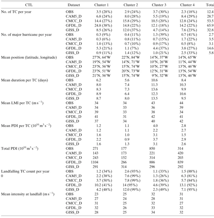
TABLE5. As inTable 3, but for the downscaled simulations for the control run. Percent values (in parentheses) represent the pro-portions, within each cluster, of total tropical cyclone counts that reached a given intensity at some points of its lifetime or made landfall at least once.
CTL Dataset Cluster 1 Cluster 2 Cluster 3 Cluster 4 Total No. of TC per year OBS 3.5 (28%) 2.9 (24%) 3.7 (30%) 2.3 (18%) 12.4
CAM5_D 6.8 (24%) 8.0 (28%) 5.5 (19%) 8.4 (29%) 28.7 CMCC_D 14.4 (27%) 15.8 (29%) 10.5 (20%) 12.8 (24%) 53.5 GFDL_D 24.8 (38%) 14.8 (22%) 12.1 (18%) 14.2 (22%) 65.9 GISS_D 8.5 (26%) 12.0 (37%) 4.7 (14%) 7.6 (23%) 32.8 No. of major hurricane per year OBS 0.3 (9%) 0.4 (11%) 1.3 (39%) 0.7 (41%) 2.7 CAM5_D 0.3 (6%) 0.8 (11%) 0.7 (15%) 1.7 (22%) 3.5 CMCC_D 1.0 (13%) 0.7 (10%) 0.9 (17%) 0.5 (8%) 3.1 GFDL_D 5.3 (21%) 1.1 (7%) 4.4 (37%) 3.8 (27%) 14.6 GISS_D 0.9 (11%) 1.4 (12%) 1.0 (21%) 2.5 (33%) 5.8 Mean position (latitude, longitude) OBS 278N, 648W 228N, 848W 148N, 378W 148N, 658W
CAM5_D 198N, 548W 148N, 718W 108N, 268W 118N, 448W CMCC_D 238N, 568W 158N, 748W 108N, 278W 138N, 468W GFDL_D 238N, 518W 208N, 738W 128N, 318W 138N, 548W GISS_D 218N, 568W 158N, 748W 98N, 328W 138N, 468W Mean duration per TC (days) OBS 6.2 5.6 10.6 8.4
CAM5_D 8.0 7.4 11.3 10.3 CMCC_D 8.3 7.3 13.6 9.9 GFDL_D 8.9 6.4 12.3 10.6 GISS_D 8.7 8.0 13.5 9.5 Mean LMI per TC (m s21) OBS 34 34 43 44
CAM5_D 34 33 36 39
CMCC_D 39 33 38 34
GFDL_D 41 31 42 41
GISS_D 37 34 40 42
Mean PDI per TC (1010m3s22) OBS 1.2 1.1 4.0 2.8
CAM5_D 1.2 1.1 2.2 2.7 CMCC_D 1.6 1.0 3.1 1.5 GFDL_D 2.2 0.9 3.7 2.9 GISS_D 1.6 1.3 3.1 2.6 Total PDI (1010m3s22) OBS 271 177 850 314
CAM5_D 143 173 221 420 CMCC_D 243 152 314 203 GFDL_D 1104 266 886 839 GISS_D 291 314 296 292 Landfalling TC count per year OBS 1.2 (34%) 2.6 (93%) 1.1 (33%) 1.5 (88%) 0 CAM5_D 2.2 (38%) 7.6 (99%) 1.3 (26%) 6.3 (81%) CMCC_D 3.7 (50%) 7.8 (99%) 1.8 (36%) 5.7 (84%) GFDL_D 10.2 (41%) 14 (95%) 4.6 (39%) 13.1 (92%) GISS_D 4.2 (48%) 12.0 (99%) 2.3 (49%) 7.1 (95%) Mean intensity at landfall (m s21) OBS 23 25 32 31
CAM5_D 27 24 28 31
CMCC_D 31 25 32 27
GFDL_D 32 26 33 32
GFDL_D, 56% for CMCC_D, and 52% for CAM5_D. However, most of the downscaled models overestimate the proportion of tropical cyclones in clusters 2 and 4 and underestimate the proportion of tropical cyclones in clusters 1 and 3. The effect of this bias will be dis-cussed below.
A clear advantage of the downscaled simulations is that they are able to produce a realistic proportion of hurri-canes (not shown here) and major hurrihurri-canes (Table 5). In the observations the number of tropical cyclones that become major hurricanes (Saffir–Simpson categories 3– 5) is substantially weighted toward the southernmost systems (Table 5), with approximately 40% of tropical cyclones in clusters 3 and 4 becoming major hurricanes, while only 12% of storms in clusters 1 and 2 reach those categories. Three of the four downscaled models have a fairly realistic percentage of tropical cyclones in-tensifying into major hurricanes (CAM5_D, GFDL_D, and GISS_D), and these models simulate a higher rate of intensification for the southernmost tropical cyclones. However, for these models, the difference between the northernmost and southernmost tropical cyclone inten-sification rates is not as high as in observations. For ex-ample, in the case of GFDL_D, 37% and 27% of storms in clusters 3 and 4, respectively, reach major hurricane intensity, in contrast with 21% and 7% of storms in clusters 1 and 2, respectively (Table 5). For models CAM5_D and GISS_D, the rate of tropical cyclones that reach major hurricane intensity is highly underestimated, and there is a much weaker contrast between the north-ernmost and southnorth-ernmost tropical cyclone intensifi-cation rates. CMCC_D has reasonable rate of storms reaching major hurricane intensity but has a similar per-centage of major hurricanes among the four clusters, therefore underestimating the percentage in all clusters (10%–17%; seeTable 5).
In observations, the majority of category 5 hurricanes occur in clusters 3 and 4 (Kossin et al. 2010). This is also the case for GFDL_D and GISS_D. Of the 39 (12) cat-egory 5 hurricanes that have been simulated by GFDL_D (GISS_D), 32 (8) are in clusters 3 and 4. The number of category 5 hurricanes simulated in the other two models is too low to be analyzed here.
cause the downscaling technique does include the early stages of extratropical transition but does not reclassify the storms as extratropical.
As mentioned above, in observations the LMI follows a bimodal distribution with a higher mean intensity for the southernmost tropical cyclones than in the north-ernmost ones. All the downscaled models, with exception of CMCC_D, manage to reproduce this characteristic. CAM5_D, GFDL_D, and GISS_D have a mean LMI for the northernmost tropical cyclones between 34 and 36 m s21, while for the southernmost cyclones it varies between 38 and 42 m s21. Even if there is a more pro-nounced contrast in the observations, the downscaled models are able to simulate the differences in intensity between the northernmost and southernmost tropical cyclones, which is a very encouraging result.
Table 5presents the mean PDI per tropical cyclone for each cluster. In observations, the mean PDI is clearly higher for the southernmost tropical cyclones (clusters 3 and 4) compared with the northernmost ones (clusters 1 and 2). All the downscaled models also reproduce this difference (Table 5). However, the downscaled models tend to underestimate the mean PDI of the southernmost tropical cyclones. Although in the simulations, the mean PDI varies between 2.2 3 1010(CAM5_D) and 3.73 1010m3s22(GFDL_D) and for cluster 4 it varies between 1.53 1010(CMCC_D) and 2.93 1010m3s22(GFDL_D), in observations the mean PDI values are 4.0 and 2.83 1010m3s22, respectively. The mean PDI per tropical cy-clone depends on the tropical cycy-clone duration and in-tensity. Because all the downscaled models overestimate the storm duration and underestimate the storm intensity, the bias in mean PDI per storm can be attributed to the bias in storm intensity (Table 5). In observations, cluster 3 tropical cyclones have the highest value of mean PDI (Table 5) and hence are potentially more dangerous when reaching the coasts. Except for CAM5_D, the down-scaled models reproduce the higher mean PDI of cluster 3 tropical cyclones (Table 5). This is an important result, because it is fundamental to be able to simulate well the characteristics of the most potentially destructive storms. Similarly, for the observed total PDI (Table 5), cluster 3 has a much higher value than the others, reaching
8503 1010m3s22with the second highest value (3143 1010m3s22) occurring in cluster 4. Unfortunately, except CMCC_D, none of the downscaled models reproduces this characteristic, because of an underestimation of the intensity and wrong proportion of tropical cyclones per cluster (Table 5). For GFDL_D, cluster 1 presents the highest total PDI, overestimating of intensity and pro-portion (Table 5) of the total PDI in that cluster. For CAM5_D and GISS_D, clusters 4 and 2 are respectively the ones with the highest total PDI among all clusters, overestimating the proportion of tropical cyclones in those clusters.
c. Landfalls
Besides specific intensity, frequency and duration characteristics, Kossin et al. (2010) showed that ob-served clusters present different landfall properties. To obtain the points of landfall for each model, we first used a very high-resolution land–sea mask based on obser-vational data in order to include all small islands. Then we interpolated each track from 6-hourly positions to 15-min increments using cubic splines. Finally, for each interpolated track, whenever the storm location is over land—and on the previous time step the storm was over water—this is defined as a landfall. Characteristics of landfalls are very important in climate studies, as land-falling storms can impact the coastal population. There-fore, the ability of climate models to reproduce landfall distribution and robust projections of changes in landfall frequency is essential for impact studies.
Table 5presents the number and proportion of land-falls in observations and downscaled simulations for each cluster. The downscaled simulations have very re-alistic landfall proportions compared to observations, with most of the tropical cyclones in clusters 2 and 4 making landfall at least once, while the landfall pro-portion in clusters 1 and 3 is much lower because of the eastern genesis location of the last two clusters.
The clusters differ not only in landfall proportions but also more importantly on the geographic position of their landfalls (as shown in observations in right panels ofFig. 1). Observed and downscaled tropical cyclones in cluster 1 make landfall along the eastern U.S. and Canada coasts. Cluster 2 landfalls are largely confined to the Gulf of Mexico, western Caribbean, and Antilles, whereas cluster 3 landfalls occur over the eastern U.S. and Canada coasts and the Antilles. Finally, cluster 4 has the landfalls in the An-tilles and the Mexico and Central America coasts. There is a much higher proportion of tracks making landfall in the eastern U.S. and Canada coasts in the downscaled models compared to the observations for all the clusters.
Another important characteristic to consider is the ability of models to simulate the intensity of storms at
landfall, which is shown inTable 5for observations and downscaled models for each cluster. The southernmost tropical cyclones have higher intensity at landfall for the observations and in two of the downscaled models (CAM5_D and GISS_D). In contrast, CMCC_D and GFDL_D present very similar intensities at landfall for all clusters. The reasons for these differences should be addressed in a future study.
d. Seasonality
The seasonality of downscaled simulations for all storms in the basin is very similar to observations (not shown). However, as shown in Fig. 9, none of the downscaled models is able to reproduce the observed seasonal distribution per cluster. Also, as inFig. 7, the large error bars show that the models have very large spread among them. For GFDL_D (Fig. 9c) and GISS_D (Fig. 9d), one cluster is prevalent: cluster 1 is highly dominant for GFDL_D in the early and the middle part of the season, while for GISS_D cluster 2 has larger values over the whole season. In those two cases, the dominant cluster has also a largely overestimated pro-portion (Table 5). For CAM5_D (Fig. 9a) and CMCC_D (Fig. 9b), there is a different leading cluster in each part of the season, but these are different from observations.
It is interesting to note that, except CAM5_D, the seasonal cycle of explicit versus downscaled simulations is completely different (cf.Figs. 7band9a). Moreover, while GFDL_E had a realistic seasonal cycle per cluster (Fig. 7d), when using the downscaling technique, the seasonal cycle of GFDL_D is degraded (Fig. 9c). The biases of this downscaled model cannot be attributed to the large-scale conditions as these two simulations share the same large-scale environment. The seeding process, as well as the seeding timing, could be a possible ex-planation for the differences between the seasonality in explicit and downscaled simulations. As mentioned above, one drawback of the downscaling method is that there is no link with the timing of the African easterly waves; this could be one of reasons for seasonality biases of the downscaled simulations, especially in the case of the nonrealistic timing of genesis of cluster 3 storm genesis. This result clearly shows a limitation of the downscaling technique that should be further improved. In summary, the downscaled models generally simu-late better the cluster separation and characteristics, such as duration, intensity, PDI, and landfalls frequency, when compared with explicit models; in particular, the storms reach the intensity of hurricanes and major hur-ricanes. However, there are some biases remaining. For example, some of the downscaled models are not able to reproduce the bimodal distribution of intensity between the northernmost and southernmost tropical cyclones
and all downscaled models had problems simulating the seasonality of cluster memberships.
5. Future changes in North Atlantic tracks a. Frequency
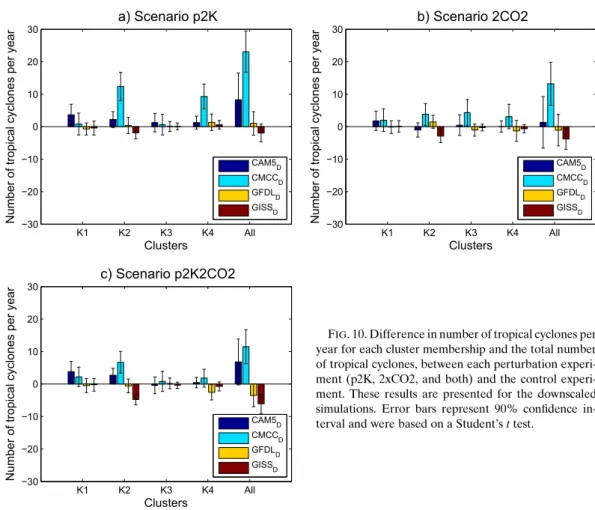
Because of the low number of tropical cyclones in most of the explicit models, future changes in tropical cyclone activity are only examined for the downscaled models. The histograms inFig. 10show the difference in the number of tropical cyclones per year for each of the three perturbation experiments (p2K5 2-K increase in SST, 2CO25 2 3 CO2, and p2K2CO25 2-K increase in
SST and 23 CO2). The results are shown for the cluster
memberships, as well as the total number of tropical cyclones. Error bars indicate the 90% confidence in-terval on the differences. A Student’s t test was realized in order to get the confidence intervals.
The changes in the total number of tropical cyclones per year show large differences among the four down-scaled models, as well as the three idealized scenarios. CAM5_D and CMCC_D both show an increase of the
total number of tropical cyclone per year, for all the scenarios. One reason for that might be that, if the same seeding rate is kept between the present and future simulations, under future conditions the environment might more favorable so the number of tropical cyclones might get higher. However, for CAM5_D, the results are not statistically significant. In the case of CMCC_D, there is a major significant increase in tropical cyclone fre-quency for all scenarios: 145% (p2K;Fig. 10a),127% (2CO2;Fig. 10b), and122% (p2K2CO2; Fig. 10c), re-spectively. In contrast, the other downscaled models tend to present weaker changes and often differ in sign. For the p2K scenario (Fig. 10a), GFDL_D and GISS_D show significant decreases in frequency of tropical cy-clones per year with29% and 26%, respectively. For the 2CO2 (Fig. 10b) and p2K2CO2 (Fig. 10c) scenarios, GFDL_D and GISS_D also present decreases in trop-ical cyclone frequency; however, changes in GFDL_D are not statistically significant. GISS_D has small de-creases of number of tropical cyclones per year with 23% for 2CO2 and 26% for p2K2CO2. Yoshimura and Sugi (2005)showed that frequency changes in the