HAL Id: inserm-00129694
https://www.hal.inserm.fr/inserm-00129694
Submitted on 9 Feb 2007HAL is a multi-disciplinary open access archive for the deposit and dissemination of sci-entific research documents, whether they are pub-lished or not. The documents may come from teaching and research institutions in France or
L’archive ouverte pluridisciplinaire HAL, est destinée au dépôt et à la diffusion de documents scientifiques de niveau recherche, publiés ou non, émanant des établissements d’enseignement et de recherche français ou étrangers, des laboratoires
Spherical harmonics based intrasubject 3-D kidney
modeling/registration technique applied on partial
information.
Jean-Louis Dillenseger, Hélène Guillaume, Jean-Jacques Patard
To cite this version:
Jean-Louis Dillenseger, Hélène Guillaume, Jean-Jacques Patard. Spherical harmonics based intrasub-ject 3-D kidney modeling/registration technique applied on partial information.. IEEE Transactions on Biomedical Engineering, Institute of Electrical and Electronics Engineers, 2006, 53 (11), pp.2185-93. �10.1109/IEMBS.2004.1403511�. �inserm-00129694�
Spherical harmonics based intra subject 3D kidney
modeling/registration technique applied on partial information
Jean-Louis Dillenseger*,** H´el`ene Guillaume*,** Jean-Jacques Patard***
From:
* INSERM, U642, Rennes, F-35000, France;
** Universit´e de Rennes 1, LTSI, Rennes, F-35000, France; *** CHU Rennes, Service d’Urologie, Rennes, F-35000, France; Corresponding author:
Jean-Louis Dillenseger
Laboratoire Traitement du Signal et de l’Image, INSERM U642, Universit´e de Rennes 1,
Campus de Beaulieu,
263, Avenue du G´en´eral Leclerc, F-35042 Rennes Cedex, France.
tel: +33 (0)2 23 23 55 78 fax: +33 (0)2 23 23 69 17 email: Jean-Louis.Dillenseger@univ-rennes1.fr
1
This material is presented to ensure timely dissemination of scholarly and technical work.
HAL author manuscript inserm-00129694, version 1
HAL author manuscript
Abstract
This paper presents a 3D shape reconstruction/intra-patient rigid registration technique used to establish a Nephron-Sparing Surgery preoperative planning. The usual preoperative imag-ing system is the Spiral CT Urography, which provides successive 3D acquisitions of comple-mentary information on kidney anatomy. Because the kidney is difficult to demarcate from the liver or from the spleen only limited information on its volume or surface is available. In our paper we propose a methodology allowing a global kidney spatial representation on a spherical harmonics basis. The spherical harmonics are exploited to recover the kidney 3D shape and also to perform intra-patient 3D rigid registration. An evaluation performed on synthetic data showed that this technique presented lower performance then expected for the 3D shape recovering but exhibited registration results slightly more accurate as the ICP technique with faster computation time.
Keywords
Nephron-Sparing Surgery, 3D modeling, 3D rigid registration, spherical harmonics.
1
Introduction
Renal cancer represents 2 to 3% of solid tumors and is the third most frequent urological cancer. Today, renal tumors are detected more and more precociously. Such tumors are usually measuring less than 4 cm, so that a nephron sparing surgery can be considered instead of a total nephrectomy [1, 2].
For achieving this nephron sparing technique, the surgeon needs a precise preoperative planning in order to delineate as accurately as possible the renal carcinoma and to specify its relations with the renal arterial, venous and collecting system anatomy.
The CT uroscan is the classical preoperative examination. It consists of four time spaced 3D acquisitions, which provides complementary information about the kidney anatomy. The first acquisition is realized without injection of contrast medium and informs the surgeon about intern morphology of the patient. The second one, taken just after a contrast medium
injection, reveals the renal arterial system. Obtained just a time later, the third acquisition presents the venous and renal parenchyma vascularization. These two acquisitions give also information about the nature and the location of the renal carcinoma. About ten minutes later on the last acquisition the collecting system is enhanced. Since information from these acquisitions is of a complementary nature, it is useful for the surgeon to integrate this infor-mation within a unique spatial volume. The first step in this integration process is to bring the different acquisitions into spatial alignment. This procedure is referred as registration. This information merging after registration helps to define precisely the kidney anatomy and so to establish the surgical planning. During the operation, the surgeon handles the whole kidney. But if the kidney presents on the preoperative CT volumes a good contrast with most of the organs however it is really difficult to demarcate from the liver or the spleen (no identified limits, similar gray levels and similar behavior after injection of contrast agent). In the worst cases, up to 30 % of the kidney surface can be overlapped with other organs but usually the joint surface is less than this proportion. Only limited information on the kidneys volumes or they external surfaces is available. It is therefore important to recover on the preoperative data the entire anatomy by a modeling technique. The 2 goals of our study were: the developments of techniques allowing the reconstruction of the whole kidney shape from missing data and the registration of two kidney shapes presenting missing data.
Several registration techniques have been studied (see [3, 4] for surveys on registration). The choice of a specific technique is generally correlated to particularities of the data to register:
• In our case of a time spaced CT volumes acquisition, a 3D-3D, monomodal, intra subject
registration technique should be used.
• We acknowledged the kidney moved within the abdomen between two acquisitions but
that its shape was not deformed during the acquisitions even during the respiratory movements. This hypothesis allowed us to choose a rigid kidney-centered registration technique: only the kidneys (and not the whole body) present on the several acquisitions are matched one to the others. The registration technique is so divided into two stages: the kidney segmentation followed by the matching itself.
• We did not dispose of extrinsic surgically placed landmarks. Additionally, selection of
intrinsic landmarks is not easy and operator dependant. The registration technique has to be based on the object spatial properties (volume or surface).
• On some places, the kidney boundaries or volume can not be demarcate from other
organs. The registration technique should so match some partial available common information. The easiest common reachable information between all the modalities is the kidney outer surface which can be segmented by simple thresholding methods. The examination of the similar information between the modalities to match led to consider the partial surface registration technique family.
Within this family of registration technique, several algorithms can be classified according to the surface representation and to similarity criterion [4].
One of the simplest and efficient technique allowing rigid registration on incomplete points sampled surfaces is the Iterative Closest Points (ICP) algorithm [5]. The primitive used for registration are the surface points or the polygonal approximation of the surface. The similarity criterion is a distance to minimize between a pair of surface points or between a point and a surface. ICP (or one of its variants [6]) is generally considered as one of the reference standard registration method.
Other surface representations can also be used for registration: features (crest lines [7], etc.), local surface model [8],... However, none of them are able to recover the missing infor-mation. More global shape descriptions can also be used for the registration purpose. For example, the shape description by its 3D moments [9] is a widespread registration technique but it is also ineffective in our case. Other global spatial descriptions should be used.
The object spatial properties can be expressed by spherical harmonics [10, 11, 12]. These authors mainly used the spherical harmonics to perform shape analysis. Burel and Henocq [13, 14] showed that this description is not only suitable for surface modeling but also for registration. However, the work presented in their papers had several limitations: the reg-istration framework was only illustrated on a extracted rigid shape (a dried vertebra), no comparisons with other registration techniques were performed and the decomposition of an object into the spherical harmonics basis was only performed from a regular sampling of the
whole volume or surface information. A technique allowing the complete shape description by spherical harmonics decomposition even in the presence of missing information would comply with our twofold objective: surface modeling and registration.
The objectives of our paper is to adapt the spherical harmonics based registration principle to our specific medical application presenting missing information, to evaluate the influence of the parameters of this method and to compare it to ICP.
The paper is organized as follows. In section 2 the principle of the spherical harmon-ics decomposition is presented including the spherical harmonharmon-ics estimation in the face of missing information and the proposed registration technique. Then, the spherical harmonics decomposition adaptation to 3D/3D kidney registration and modeling is explained. Finally, experimental results on synthetic realistic data are used to evaluate our methodology.
2
Spherical harmonics
The spherical harmonics are functions defined on the unit sphere. They were developed in quantum mechanics [15] [16] and are also used in shape recovery and modeling.
2.1 Definitions
Spherical harmonics are solutions of Laplace’s equation expressed in a spherical coordinate system as following: Ylm(θ, ϕ) = (−1)m r 2l + 1 4π s (l − m)! (l + m)!P m
l (cos θ)eimϕ (1)
where :
Ym
l are the spherical harmonics indexed by l, the harmonic degree, which vary from 0 to L, with L, the decomposition level, and −l < m < l.
θ the spherical coordinate angle to z, (0 ≤ θ ≤ π).
ϕ the spherical coordinate angle within the xy plane, (0 ≤ ϕ ≤ 2π). Pm
l the Legendre polynomials.
2.2 Surface modeling
Spherical harmonics constitute a basis of orthogonal functions, which ensures the uniqueness of the decomposition of a shape over the unit sphere. So, any finite energy and differentiable function defined over the sphere can be approximated by a linear combination of spherical harmonics: f (θ, ϕ) = ∞ X l=0 +l X m=−l Clm· Ylm(θ, ϕ) (2)
where f (θ, ϕ) is in our case the surface of a 3D object (the shape) described in the spherical coordinate system and the Clmcoefficients correspond to the shape coordinates in the spherical harmonics basis.
If a surface is regularly sampled over the spherical coordinate system, its modeling consists in finding the Cm
l coefficients for its specific shape. They can be obtained by the projection of the sampled points onto the basis of spherical harmonics and more formally by using the inner product of the function f with the vectors of the spherical harmonics basis:
Clm=< f (θ, ϕ), Ylm(θ, ϕ) >= p X i=1 q X j=1 f (θi, ϕj) · Ylm(θi, ϕj) · ∆ϕ · sin θi· ∆θ (3) where:
f (θi, ϕj) are the known sampled function points. p = number of samples in θ.
q = number of samples in ϕ. ∆θ and ∆ϕ sampling steps.
2.3 Surface modeling with missing information
When the shape presents missing information, we can no longer compute the harmonic co-efficients by linear integration like in equation (3) for the reason that some data for certain spherical coordinates (θi, ϕj) are missing.
Because the representation is in the form of a linear combination of fixed basis functions, one solution consists in estimating the coefficients from the accessible information by a least
squares fitting technique.
If we assume that the surface is approximated by a reconstruction up to a decomposition level L (L 6= ∞).
Let ¯f be a column vector where each line corresponds to a known surface point: f (θk, ϕk). Let Y be the matrix of spherical harmonics, where each line corresponds to a known surface point: Y = ¯ ¯ ¯ ¯ ¯ ¯ ¯ ¯ ¯ ¯ ¯ ¯ ¯ Y0 0(θ1, ϕ1) Y1−1(θ1, ϕ1) . . . YLL(θ1, ϕ1) Y0 0(θ2, ϕ2) . .. .. . ... Y0 0(θn, ϕn) Y1−1(θn, ϕn) . . . YLL(θn, ϕn) ¯ ¯ ¯ ¯ ¯ ¯ ¯ ¯ ¯ ¯ ¯ ¯ ¯ Let ¯C be the corresponding vector of harmonic coefficients:
¯ C = ¯ ¯ ¯ ¯ ¯ ¯ ¯ ¯ ¯ ¯ ¯ ¯ ¯ C0 0 C1−1 .. . CL L ¯ ¯ ¯ ¯ ¯ ¯ ¯ ¯ ¯ ¯ ¯ ¯ ¯ Equation (2) can be written as:
¯f = Y · ¯C (4)
The surface modeling consists in finding the vector ¯C which minimizes the distances between the surfa5ce points ¯f and these estimated by Y · ¯C:
d2 = (¯f − Y · ¯C)2 (5)
The minimization of d2 = (¯f − Y · ¯C)2 can be solved by a generalized inverse (or
pseudo-inverse) procedure, like:
¯
C = (YT· Y)−1· YT· ¯f (6)
2.4 Rotation
We express a 3D rotation with 3 Euler angles using the ”y-convention”: a first rotation by an angle α about the z axis, the second by an angle β about the y axis and the third by an angle γ about the z axis again.
If we perform a rotation R(α, β, γ) on the shape, this will affect the Cm
l coefficients by the following relationship [15] [13]:
Clm(α, β, γ) = l X n=−l Dlmn(α, β, γ)Cln (7) With : Dlmn(α, β, γ) = e−iγn· dlmn(β) · e−iαm and dlmn(β) = min(l+n,l−m)X t=max(0,n−m) (−1)t p (l + n)!(l − n)!(l + m)!(l − m)! (l + n − t)!(l − m − t)!(t + m − n)!t! µ cosβ 2 ¶(2l+n−m−2t)µ sinβ 2 ¶2l+m−n If we know the Cm
l coefficients before the rotation, expression (7) determines the coeffi-cients after rotation: Cm
l (α, β, γ).
2.5 Registration method
A registration methodology has been described in [13]. This technique needs no correspon-dence between points and is not an iterative research. It is based on the tensors properties. The 3D object (its shape) is decomposed on the spherical harmonics basis where the coeffi-cients are calculated according to equations (3) or (6).
Translation: Because the coordinate system is object centered, the decomposition of a shape is almost invariant in translation. Thus, the translation registration consists only in
realigning the shapes centers of gravity (see the paragraph ”Surface extraction and translation estimation” on the Results section).
Rotation: Spherical harmonics are used for rotation registration. The main idea of this method is the following: for both shapes we determine a rotation that brings the shapes to a standard reference orientation characterized by some specific constraints on the Cm l coefficients. These two rotations are then used to realign the two shapes.
Rotation to a standard reference orientation. Since we have three degrees of freedom, three
constraints are necessary (for example cancel one complex coefficient and the imaginary part of another one, further constraints on the signs of some coefficients can be added to resolve some ambiguities). Many possibilities exists but when the constraints are imposed on the first or second order orthogonal subspace, explicit equations can be written and the angles com-puted using trigonometric functions. For a question of precision, the constraints are generally imposed on the ε2 orthogonal subspace which basis is: {|Y2−2i, |Y2−1i, |Y20i, |Y21i, |Y22i}.
The reference orientation corresponds to the following constraints: C1 2(α, β, γ) = 0 C2
2(α, β, γ) real positive and maximal
Re{C1
1(α, β, γ)} ≥ 0 and Im{C11(α, β, γ)} ≥ 0
(8)
The resolution of these constraints allows to determine an unique rotation (α, β, γ) (see [13] for the resolution of the constraints) which brings a shape to a standard reference orientation.
Registration. The principle of the registration of two shapes by spherical harmonics
con-sists then in:
1. Determining the orientation of each surface with regard to the shape dependent reference orientation by solving the equation (7) with the constraints mentioned in equation (8).
For shape 1, the resolution of the constraints leads to determine (α1, β1, γ1). These
angles constructs the rotation matrix R01 which brings the shape 1 to its reference
orientation.
For shape 2, the resolution of the constraints leads to determine (α2, β2, γ2) and so R02.
2. Using R01 and R02, the rotation matrix R21 which realigns the shape 2 on the shape
1 is given by:
R21= R02T· R01 (9)
3
Results
The purpose of this section was to evaluate the modeling/registration technique. The choice of the test data were one of the fundamental issues for any evaluation. The next subsection presents the data we were using for the subsequent tests. Three aspects were then analyzed: 1) Adaptation of the spherical harmonics decomposition and more specifically the spherical harmonics coefficients estimations to our specific medical urologic application, 2) Performance of data modeling and 3) Accuracy of the registration in comparison to another standard reference method.
3.1 Data
Basically, two fundamental choices were available: synthetic and real data. Reminding the three aspects described above, aspect 1 (the adaptation of the technique to our problematic) needs real data, by opposite the evaluations of aspects 2 (data modeling) and 3 (registration) must be performed on synthetic data. We chose to create synthetic data from real one. For each test, surface samples were collected on real data. From these samples, known synthetic transformations like information cutting or rotations were performed in order to create the data used for the methodologies evaluations.
The real data was provided by a clinical 3D abdominal CT database (35 slices of 512x512 pixels, the pixel resolution is 0.68 mm with a slice thickness and inter-slices spacing of 5 mm). In a first step, the database is restored isotropic by interpolation. In a second step, one kidney is segmented semi-automatically (region-growing and manual adjustments). Finally our test database contains a extracted kidney within a 512x512x256 voxels volume with a resolution of 0.68 mm per isotropic voxel size.
Surface extraction and translation estimation: The kidney surface has to be sampled over the spherical coordinate system. Seen from the center of gravity, the kidney shape is almost closed and convex (star-shaped). However if this characteristic cannot been fulfilled, the study performed by Brechb¨uhler and al. [11] shows that this limitation can be overcome. We use an iterative framework to extract and sample the kidney surface and also to determine the translation between the kidneys from the several acquisitions. In a first step, a seed point is manually placed within the kidney (approximatively on the kidney center). From this point rays are cast towards the surface for each direction (θi, ϕj). Each ray travels through the volume voxels until it detects the surface [17] measuring then the radial distance
r1ij from the seed point to the surface. This ray casting scheme can take the voxel partial
volume into account in order to detect the surface on a subvoxel accuracy [18]. In a second step, the center of gravity of the detected surface points is computed and serves as new seed point for a new surface sampling. This procedure is iterated until the center of gravity location is converging (only a few iterations are necessary). At the end of this iterative framework, we have at our disposal the center of gravity which is used to estimate the translation and a regular surface sampling within the spherical coordinate system. Figure 1 left shows the extracted surface after filling the space between points samples by polygons.
Object rotation: We express a 3D rotation as a unique rotation φ around a specific axis characterized by its normalized vector A(xA, yA, zA). This rotation gives a rotation matrix R21. The rotated object is sampled as following: the radial distance r2ij from the center of
gravity to the rotated surface along the direction (θi, ϕj) is estimated by casting a ray on the original data along the direction (θ0
i, ϕ0j) = R21−1· (θi, ϕj).
On the following sections, the object before rotation will be mentioned as ”Object 1” and as ”Object 2” after rotation.
Object truncation: In order to validate the surface modeling and registration method on missing data, we eliminate points on the surface. These points are chosen as following: around a specific direction B(θB, ϕB) we fix a truncation angle ξ which generates a cone. Each surface sample which coordinates belong to this cone is eliminated (figure 1 right).
We suppose that even if the kidneys move because of the breathing, they remain in contact with the other organs within the same area. For this reason, we took attention to realize the suppression on the rotated object at the same place as for the original object. This can be done by rotating B: B0(θ0B, ϕ0B) = R21· B(θB, ϕB) on ”Object 2”.
3.2 Spherical harmonics coefficients estimation
This section presents the spherical harmonics decomposition adaptation to our 3D/3D kidney registration and modeling problem.
Both objectives, reconstruction and registration, are based on spherical harmonics de-composition and coefficients estimation. The main difference depends on the dede-composition level needed to perform the process. For registration only the decomposition level L=2 is necessary but for reconstruction higher decomposition levels are needed to finely describe the shape. In this section, we examine the spherical harmonics coefficients estimation methods and parameters.
3.2.1 Harmonics coefficients computation
We consider 3 cases:
1. The coefficients computation by projection of the sampled points onto the basis of spherical harmonics according to the equation (3). The volume is here regularly sampled and the information is complete. This computation is mentioned as ”linear integration” afterwards in the paper.
2. The estimation of coefficients by least squares fitting on complete and regularly sam-pled data. However, the estimation of coefficients for some harmonic degree l could require to compute equation (6) with a decomposition level L higher as l. This compu-tation is mentioned as ”complete least squares” afterwards in the paper. If needed the decomposition level l is specified.
3. Last, we estimate the coefficients by least squares fitting, on the same data, but after points suppression for different truncation angles. This computation will be mentioned
as ”incomplete least squares” afterwards.
3.2.2 Decomposition and reconstruction, the influence of spatial sampling
Spherical harmonic decomposition and reconstruction with several decomposition levels have been performed on the extracted kidney (figure 2). The reconstruction using the harmonic coefficients till a decomposition level L=2 shows the shape used for the registration.
Concerning the spatial sampling, it could be demonstrated that for a specific decomposi-tion level L the sampling steps ∆θ and ∆ϕ < 2L−1π preserve Shannon’s sampling theorem for equation (1). However the shape spatial frequency should also be taken into account.
For our specific data, we examine the accuracy of the harmonic coefficients estimation with increasing ∆θ and ∆ϕ sampling steps. The coefficients estimated with the finest sampling steps (∆θ = ∆ϕ = 0.5 degree) are considered as reference. The coefficients estimation accuracy for greater sampling steps is measured by computing the relative errors between the estimated coefficient ˆCm
l and the reference ones Clm: error(%) = ¯ ¯ ¯ ¯ ˆ Cm l −Cml Cm l ¯ ¯ ¯ ¯. For L < 9, the relative errors on the Cm
l estimation can be greater than 1% with ∆θ = ∆ϕ > 5 degree. These errors are always less than 0.1% with ∆θ = ∆ϕ < 2 degree.
If not explicitly specified, we chose a sampling step of ∆θ = ∆ϕ = 2 degree. These steps allow sampling 16380 surface points and appear to be a good compromise between accuracy and computation speed. The harmonic coefficients computation time in the linear integration case is about 0.25s for L = 2 and 0.96s for L = 9 on a classical PC (AMD Athlon 2200+, 1Mo RAM).
3.2.3 Linear integration vs. complete least squares
”Linear integration” and ”complete least squares” are different in the way they can compute a specific harmonic degree (eg the 2nd order coefficients). These harmonic coefficients can be computed explicitly and directly by ”linear integration” using equation (3). However, as shown on equation (4), it is possible to estimate the coefficients by least squares fitting by using some higher decomposition level L. Thus, we evaluate the influence of the decomposition level L on the harmonic coefficients estimation precision. This evaluation is performed by
computing the relative errors on the second order coefficients estimations between ”linear integration” and the ”least squares” fitting technique.
As an example the graphic on figure 3 shows the C2
2 modulus relative error between the
least squares fitting estimated coefficients and the linear integration one versus decomposition level.
Our results demonstrate that on complete data, and for a decomposition level L=6, the maximal coefficients estimation relative error is less than 0.2%, moreover the relative errors for the second order coefficients (used by the registration) are lower than 0.075%. For a decomposition level L=8, the second order coefficients estimation relative error decreases by a factor 2.
When analyzing the computation times: for the ”complete least squares” method, the coefficients are computed in around 1.72s for L=6 and in around 3.3s for L=8. This time should be compared with 0.25s for ”linear integration”.
3.3 Missing data recovering
We evaluate the missing data influence on the harmonic coefficients estimation and recon-struction. The evaluation protocol is the following:
1. On the complete data, we compute the reference harmonic coefficients Clm using ”linear integration” and make a reference reconstruction.
2. For a specific B(θB, ϕB) we generate missing data for different truncation angle ξ (0 ≤
ξ ≤ 45 degree). For each ξ, the harmonic coefficients are estimated by ”incomplete least
squares” and compared to the reference coefficients. Reconstruction using the estimated harmonic coefficients are also carried out and compared to the reference.
3. This framework is performed for 100 randomly chosen B(θB, ϕB).
The amount of missing information influence on the harmonic coefficients estimation ac-curacy is illustrated on the following case. We examine the 2nd order coefficients estimated by ”incomplete least squares” with a level L=6. The results shows that for a truncation angle ξ=20 degree which corresponds to broadly 8% of missing data, the 2nd coefficients are
estimated with a mean relative error of less than 2% with a maximum relative error less than 6%. But for higher truncation angle, the error increases rapidly (see Figure 4 for the C22 modulus estimation). This could be explained by the fact that coefficients depends on the object shape and that a high truncation misrepresents completely this shape.
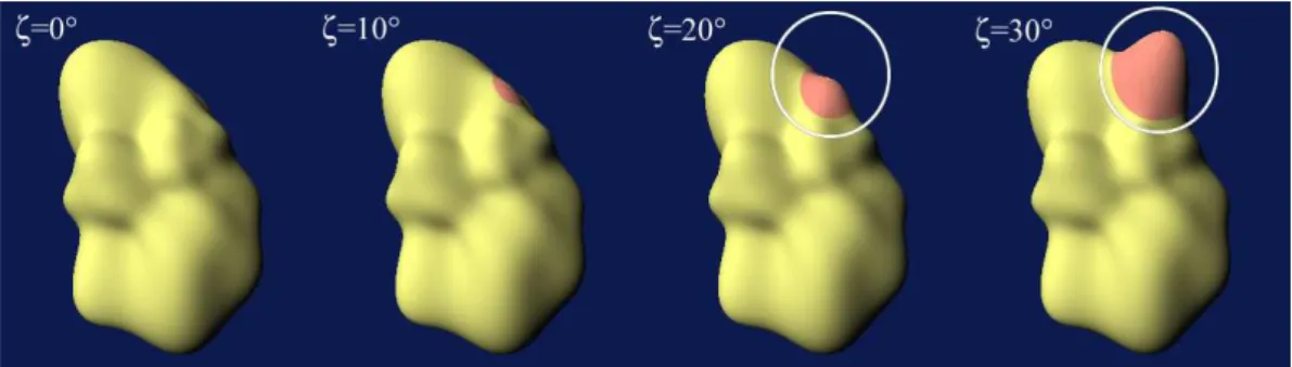
This phenomenon is also verified for the reconstruction where the errors between the reconstructed missing data and the original shape increase with the truncation angle. An example is shown Figure 5 with an ”incomplete least squares L=10” coefficients estimation and a L=10 reconstruction for different truncation angles. In this figure the truncation axis B(10 degree, 45 degree) is the same as in figure 1. The effect of the mis-reconstruction in the area around B (see circles) is clearly visible for higher ξ.
3.4 Registration
For the different following tests, we use the same registration evaluation method: the object is rotated by an angle φ around a specific axis A(θA, ϕA). φ and A give the rotation matrix R21.
The registration method estimates a rotation matrix ˆR21.
The accuracy of ˆR21 is measured in two manners:
• An error rotation matrix is created by E = R21· ˆRT21. The rotation angle deduced from
E serves as an accuracy measure. This measure is called ”angular error” and expressed in degree.
• For all the sampled object points p1i we perform a rotation by R21 (p2i = R21· p1i)
and a rotation by ˆR21 (ˆp2i = ˆR21· p1i). The maximal Euclidian distance between the
p2i and the ˆp2i serves as accuracy measure. This measure is called ”maximal distance
error” and expressed in voxel.
The proposed registration method should also be compared to other standard registration method. This standard method should be performed on the same data: rigid registration on incomplete points sampled surfaces. The Iterative Closest Points (ICP) algorithm [5] can be adapted in this way. Several variants on the ICP algorithm have been proposed differing
on the points selection and matching, pairs weighting and rejecting, the error metric and minimization [6]. Based on the previous method comparison we developed our own algorithm. The details of this algorithm can be found in the appendix.
3.4.1 Registration method validation
The object is rotated with randomly defined rotation angle φ and axis A(θA, ϕA). These rotations are then estimated using the spherical harmonics registration method (the spherical harmonics coefficients have been computed by ”linear integration”). For hundred randomly generated rotations, the maximal angular error is less than 0.11 degree and the maximal distance error is less than 0.25 voxel.
We also evaluate the registration using the spherical harmonics coefficients estimated by ”complete least squares” with several decomposition level. Table 1 shows the registration accuracy vs. ”complete least squares” decomposition levels for hundred randomly generated rotations. These results follow the same behavior as in section 3.2.3. ”Complete least squares” with L=8 has comparatively the same accuracy level as ”linear integration”. This evaluation helps us to choose L=8 as registration parameter.
3.4.2 Spherical harmonics registration methodology vs. ICP
For addressing the question of computation time (see appendix) the comparison between spherical harmonics registration methodology and ICP is performed with a ∆θ = ∆ϕ = 4 degree sampling step. In this same sampling context, the two registration methods using the spherical harmonics present a higher accuracy: 0.35 degree vs. 0.87 degree maximal angular and 0.7 voxel vs. 2.01 voxel maximal distance error (see Table 1).
This ratio is reduced for higher resolutions (∆θ = ∆ϕ = 2): 0.2 degree vs. 0.43 degree maximal angular and 0.53 voxel vs. 0.95 voxel maximal distance error but to the detriment of the ICP 1 iteration computation time (see Table 2).
3.4.3 Registration on partial information
When dealing with registration on partial information, only the method using the spherical harmonics with incomplete least squares fitting and ICP could be compared. This assessment is performed with the following parameters :
• For our method, the second order spherical harmonics coefficients are estimated by
”incomplete least squares” with L=8 and a sampling step of ∆θ = ∆ϕ = 2 degree.
• The ICP sampling step is ∆θ = ∆ϕ = 2 degree.
The evaluation protocol is the following: for a shape with several truncation angles ξ we generated randomly 100 rotations, each with a randomly generated B(θB, ϕB). The rotation estimated by both registration technique are compared to the original ones.
For ICP, the angular errors and maximal distance errors remain almost constant and are not depending on the truncation. However, for ”incomplete least squares” these errors increase with the truncation angle ξ (see figure 6). Until a truncation angle ξ ≤ 20 degree ”incomplete least squares” presents a higher accuracy than ICP but this accuracy decreases significantly for higher truncation angles.
4
Discussion
From the previous results several remarks can be formulated.
The shape description by spherical harmonics basis is performant. The estimation of the harmonic coefficients allows modeling the kidney shape with a level of details which is directly related to the decomposition level. The computation speed of the spherical harmonics decomposition is also relatively fast. The only drawback of this modeling is that the shape must be closed and convex (star-shaped) as they start from an initial radial surface function in the spherical coordinate system. However the studies performed by Brechb¨uhler [11] shows how to overcome these limitations.
The estimation of the spherical coefficients using least squares fitting gives results with an accuracy comparable to the classical linear integration with the advantage that no regular
surface sampling is needed, although a higher computation time especially for higher decom-position levels is needed. Therefore the coefficient estimation method can so be used even when the shape is not regularly described or has missing data.
The initial ambition of our work was to present and develop a method with two objectives: the reconstruction of a entire shape from missing data and the registration of two shapes presenting missing data.
The spherical harmonics decomposition provides relatively poor shape reconstruction re-sults when missing data is concentrated in one zone as in our case. The way where the missing data is completed within the spherical harmonics basis should be re-examined and some continuity constraints should be included during the coefficients estimation.
In the same condition, the rotation registration of two complete shapes (presenting no missing data) using spherical harmonics is as accurate as point/surface ICP but much faster. It allows a more accurate shape sampling when using the spherical harmonics method (and so enhancing the accuracy) compared to the ICP method.
In the case of non complete shapes, the accuracy of the spherical harmonics registration method depends directly on the amount of missing data. This is not the case of ICP where the accuracy remains more or less constant regardless the missing data amount. The results show that until a truncation angle of ξ=20 degree which corresponds to broadly 8% of missing data, the spherical harmonics method is more accurate than ICP but this accuracy decreases significantly for higher truncation angles. This amount of 8% of missing data seems to be the maximal value of the spherical harmonics registration method usability. However, the reason of this limitation seems to be the same as for the reconstruction. We hope that continuity constraints included during the spherical harmonics coefficients estimation method would enhance this usability of this method for higher degree of missing data. On the other hand, if the missing information represents less than 8% of the whole surface, spherical harmonics method remains more accurate as ICP.
In conclusion our technique is suitable for cases where missing information represents less than 8%. This situation is realistic for the left kidney because of the smaller overlapping with the spleen, dorsal muscles and intestines. For the right kidney, usually the overlapping
can be higher especially with the liver. However, more precise segmentation allows finding the kidney border even on some overlapping zones reducing so the missing information. The 8% missing information amount can then be used as threshold for the spherical harmonics registration and reconstruction method usability.
Conclusion
In this paper we presented a spherical harmonics based reconstruction and registration tech-nique which can be used to establish a Nephron-Sparing Surgery preoperative planning. This method can be directly applied on any closed and convex shape which can be described in the spherical coordinate system. In the case of a non convex shape this method can still be used after parametrization by a mapping from the surface to the unit sphere. Its particularity is that this technique can be applied on complete described information but also when the surface information is only partially available. This method has therefore two applications: the reconstruction of the whole kidney shape from partial information and the intra-patient kidney registration even if the shapes present missing data. Concerning the registration ap-plication, our method presents a slightly higher accuracy than the classical ICP algorithm but with a faster computation time. However, our method shows increasing registration or reconstruction errors when the missing information is over than 8% of the entire surface.
References
[1] A. Belldegrun, K. H. Tsui, J. B. deKernion, and R. B. Smith, “Efficacy of nephron-sparing surgery for renal cell carcinoma: analysis based on the new 1997 tumor-node-metastasis staging system,” J Clin Oncol, vol. 17, no. 9, pp. 2868–2875, 1999.
[2] A. F. Fergany, K. S. Hafez, and A. C. Novick, “Long-term results of nephron sparing surgery for localized renal cell carcinoma: 10-year followup,” J Urol, vol. 163, no. 2, pp. 442–445, 2000.
[3] J. B. Maintz and M. A. Viergever, “A survey of medical image registration,” Med Image
Anal, vol. 2, no. 1, pp. 1–36, 1998.
[4] M. A. Audette, F. P. Ferrie, and T. M. Peters, “An algorithmic overview of surface registration techniques for medical imaging,” Med Image Anal, vol. 4, no. 3, pp. 201– 217, 2000.
[5] P. Besl and N. McKay, “A method for registration of 3-D shapes,” IEEE Trans Pat Anal
Mach Intell, vol. 14, no. 2, pp. 239–256, 1992.
[6] S. Rusinkiewicz and M. Levoy, “Efficient variants of the icp algorithm,” in 3rd
Interna-tional Conference on 3-D Digital Imaging and Modeling, (Quebec, Canada), pp. 145–152,
IEEE Computer Society, 2001.
[7] J.-P. Thirion, “External points: definition and application for 3D image registration,” in
Comp. Vis. and Pat. Rec., pp. 587–592, IEEE, 1994.
[8] T. McInerney and D. Terzopoulos, “Deformable models in medical image analysis: a survey,” Med Image Anal, vol. 1, no. 2, pp. 91–108, 1996.
[9] T. L. Faber, “Orientation of 3D structures in medical images,” IEEE Trans Pat Anal
Mach Intell, vol. 10, no. 5, pp. 626–633, 1988.
[10] G. Burel and H. Henocq, “Three-dimensional invariants and their application to object recognition,” Signal Processing, vol. 45, no. 1, pp. 1–22, 1995.
[11] C. Brechb¨uhler, G. Gerig, and O. K¨ubler, “Parametrization of closed surfaces for 3-D shape description.,” Computer Vision and Image Understanding (CVIU), vol. 61, no. 2, pp. 154–170, 1995.
[12] G. Gerig, M. Styner, D. Weinberger, D. Jones, and J. Lieberman, “Shape analysis of brain ventricles using spharm,” in IEEE Workshop on Mathematical Methods in Biomedical
Image Analysis (MMBIA) 2001, (Hawaii), pp. 1171–178, IEEE Computer Society Press,
2001.
[13] G. Burel and H. Henocq, “Determination of the orientation of 3D objects using spherical harmonics,” Graphical Models and Image Processing, vol. 57, no. 5, pp. 400–408, 1995.
[14] G. Burel, H. Henocq, and J.-Y. Catros, “Registration of 3D objects using linear algebra,” in CVRMed’95 (N. Ayache, ed.), vol. 905 of Lecture Notes in Computer Science, (Nice, France), pp. 252–256, Springer, 1995.
[15] E. Wigner, Group theory and its application to quantum mechanics of atomic spectra. New York: Academic Press, 1959.
[16] J. D. Jackson, Classical Electrodynamics. New York: John Wiley, 2nd ed., 1985.
[17] J.-L. Dillenseger, C. Hamitouche, and J.-L. Coatrieux, “An integrated multi-purpose ray tracing framework for the visualization of medical images,” in 13rd conf. of the IEEE
Engineering in Medicine and Biology Society, (Orlando), pp. 1125–1126, 1991.
[18] J.-L. Dillenseger and B. Sousa Santos, “Comparison between two three-dimensional edge operators applied in a 3d navigation approach,” in Eurographics’98, (Lisbon), pp. 3.7.1– 3.7.2, 1998.
[19] T. M¨oller and B. Trumbore, “Fast, minimum storage ray-triangle intersection,” Journal
of Graphics Tools, vol. 2, no. 1, pp. 21–28, 1997.
[20] K. Arun, T. Huang, and S. Blostein, “Least-squares fitting of two 3-D points sets,” IEEE
Trans Pat Anal Mach Intell, vol. 9, no. 5, pp. 698–700, 1987.
Appendix
ICP algorithm details
We propose an adaptation of the ICP method for the rigid registration on incomplete points sampled surfaces. Based on Rusinkiewicz’s ICP methodologies comparison [6] we adjust the several variants on points selection and matching, pairs weighting and rejecting, error metrics and minimization to our issue:
• We use a points/surface registration method. In fact, a point/point registration method
is not appropriate for our purpose. Because our surfaces are sampled by a regular
angular steps, the point/point ICP method has the tendency to stick to the sampling step and estimate rotations which were a multiple of these steps.
A points/surface registration method has been chosen. ”Object 2” is described by it sampled surface points. ”Object 1” is expressed as a polygonal mesh surface created from the its sampled surface points. Both sampled points (from ”Object 1” and ”Object 2”), are exactly the same as for the spherical harmonics registration.
• The used points correspondence finding algorithm is the one referred as ”normal
shoot-ing” in Rusinkiewicz’s paper: the intersection of a ray shoots from the source point in the direction of its normal with the destination surface. This ray/polygon intersection search takes the most computer time of this method. We used M¨oller and Trumbore ray-triangle intersection method [19] which is generally described as one of the fasts.
• A constant weight is assigned to the corresponding points pairs.
• The corresponding points more than a given distance apart are rejected.
• The error metric is the mean of the Euclidian distance between corresponding points.
We used the distance mean instead of the distance sum in order to minimize the effect of the pairs rejecting.
• The minimization is performed in a classical manner by repeatedly generating a set of
corresponding points using the current transformation and finding a new transformation. The transformation between the corresponding points is computed by the SVD method [20].
The computation speed of ICP depends directly on the computation time of an iteration and the number of iterations. The iteration computing time depends directly on the number of surface points and vertexes which are directly related to the sampling steps ∆θ and ∆ϕ (see table 2 which give the mean computation time for one iteration for several sampling steps). The number of iterations depends on the initialization and the expected accuracy (minimization fractional tolerance). On our test data we make different computation time and accuracy assessments for several sampling steps. The sampling step ∆θ = ∆ϕ = 4 degree
(3962 points and 7920 vertexes) gives the best compromise between computation time (3.5 s per iteration) vs. accuracy: 0.87 degree maximal angular error and 2.01 voxel maximal distance error for hundred randomly generated rotations (see Table 2).
List of Figures
1 Visualization of the extracted kidney before (left) and after truncation (B(10 degree, 45 degree), ξ=45 degree) (right). In both cases ∆θ = ∆ϕ = 2 degree. 25 2 3D Visualization of the extracted kidney (top-left) and partial reconstructions
using the harmonic coefficients till a decomposition level L. . . 26 3 C2
2 magnitude estimation relative error vs. decomposition level . . . 27
4 C2
2 magnitude estimation mean relative error vs. truncation angle . . . 28
5 L=10 reconstructions for different truncation angle ξ . . . . 29 6 Mean angular errors vs. truncation angle for ”incomplete least squares”
spher-ical harmonics method and ICP. . . 30
List of Tables
1 Registration accuracy using harmonics coefficients estimated by ”linear inte-gration”, ”complete least squares” with several decomposition level and ICP. 31 2 ICP mean computation time for one iteration vs. sampling step . . . 32
Figure 1: Visualization of the extracted kidney before (left) and after truncation (B(10 degree, 45 degree), ξ=45 degree) (right). In both cases ∆θ = ∆ϕ = 2 degree.
Figure 2: 3D Visualization of the extracted kidney (top-left) and partial reconstructions using the harmonic coefficients till a decomposition level L.
Figure 3: C22 magnitude estimation relative error vs. decomposition level
Figure 4: C2
2 magnitude estimation mean relative error vs. truncation angle
Figure 5: L=10 reconstructions for different truncation angle ξ
Figure 6: Mean angular errors vs. truncation angle for ”incomplete least squares” spherical harmonics method and ICP.
∆θ = ∆ϕ = 2 degree max. angular error (degree) max distance error (in voxel) linear integration 0.105 0.246 least squares L=2 4.78 10.5 least squares L=4 1.18 2.51 least squares L=6 0.458 0.978 least squares L=8 0.200 0.432 least squares L=10 0.0901 0.194 ICP 0.530 0.951 ∆θ = ∆ϕ = 4 degree linear integration 0.349 0.761 least squares L=8 0.332 0.625 ICP 0.868 2.01
Table 1: Registration accuracy using harmonics coefficients estimated by ”linear integration”, ”complete least squares” with several decomposition level and ICP.
∆θ = ∆ϕ (in degree) 9 6 5 4 3 2 computation time (s) 0.03 0.11 0.65 1.5 5.2 26 max. angular error (degree) 1.741 0.971 0.799 0.868 0.592 0.530
Table 2: ICP mean computation time for one iteration vs. sampling step