HAL Id: hal-00985610
https://hal.archives-ouvertes.fr/hal-00985610
Submitted on 27 May 2014HAL is a multi-disciplinary open access archive for the deposit and dissemination of sci-entific research documents, whether they are pub-lished or not. The documents may come from teaching and research institutions in France or abroad, or from public or private research centers.
L’archive ouverte pluridisciplinaire HAL, est destinée au dépôt et à la diffusion de documents scientifiques de niveau recherche, publiés ou non, émanant des établissements d’enseignement et de recherche français ou étrangers, des laboratoires publics ou privés.
Impact of the sun patch on heating and cooling power
evaluation for a low energy cell
Auline Rodler, Joseph Virgone, Jean-Jacques Roux
To cite this version:
Auline Rodler, Joseph Virgone, Jean-Jacques Roux. Impact of the sun patch on heating and cooling power evaluation for a low energy cell. CISBAT 2013, Sep 2013, lausanne, Switzerland. 6 p. �hal-00985610�
IMPACT OF THE SUN PATCH ON HEATING AND COOLING POWER
EVALUATION: APPLIED TO A LOW ENERGY CELL
A.Rodler1; J.Virgone2; J-J.Roux3, J.L.Hubert4
1-3: CETHIL, UMR5008, CNRS, INSA-Lyon, Université Lyon 1 20 Av A. Einstein, 69621 Villeurbanne Cedex, France
4:Site EDF R&D des Renardières, Avenue des Renardières – Ecuelles, 77818 MORET-SUR-LOING Cedex, France
ABSTRACT
In the context of low energy buildings we study the impact of the incoming radiation through a window (sun patch) on the heating and cooling demand. Existing studies have shown that not considering the sun patch and fast climatic variations (Figure 4, Global radiation) can lead to important differences in energy power evaluation [1, 2, 3]. In this paper we present a 3D envelope model taking into account the minute-wise sun patch evolution. Simulation results are analysed for a low energy cell.
A numerical model has been developed in order to simulate the transient thermal behaviour, with a refined spatial (3D) and temporal (down to one minute time step) discretization of the single room. For each node of the grid, the energy conservation equations are developed. They traduce balance between short-wave and long-wave irradiations, convection, air enthalpy and three-dimensional heat conduction. The particularities of the program are that it projects the sun patch on the inner walls, the conduction is treated in three dimensions and climatic minute-wise variations are taken into account.
As main results, the surface temperature evolution, the air temperature evolution and the heating or cooling power necessary to maintain an inner air set-point temperature are calculated at each time-step. Heating or cooling power is compared to the power calculated with no sun patch incorporation (solar loads only on the floor). Conclusions are made on the importance of the integration of the sun patch and its impact on the observed results.
Keywords: sun patch, fast climatic variations, heating and cooling power, insulated cell
INTRODUCTION
Electrical energy savings has become an important issue. Among the consumption sources,
the building’s sector represents 40% of the consumed energy in France. The heating power
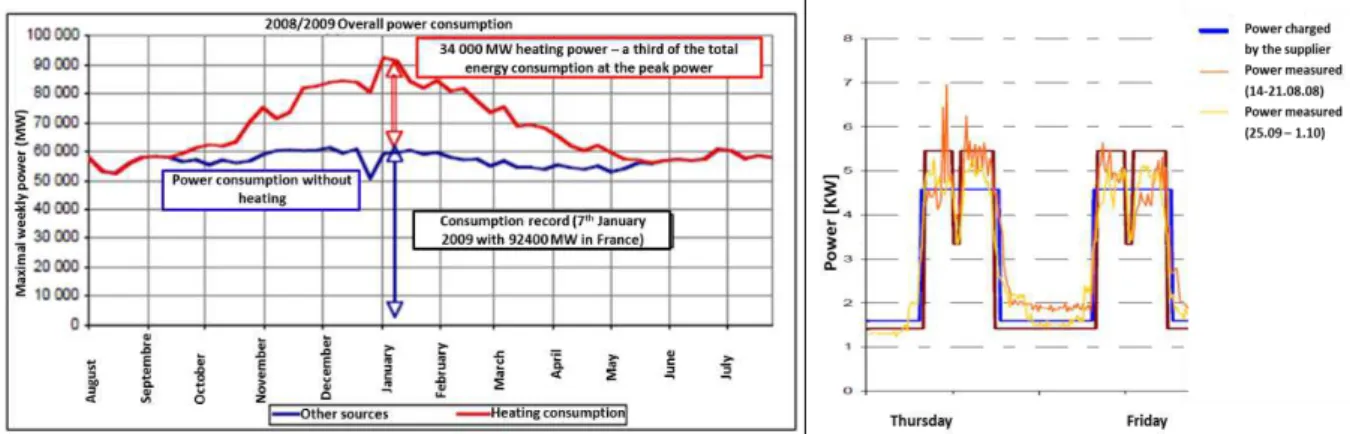
represents 2/3 of the total power consumption of the buildings sector [4] so that, in January 2009 for example, heating power represented a third of the total maximal power demand [5] (Figure 1). Therefore, a particular attention is given to the development of low energy buildings, which are strongly insulated and require less energy demand.
Very often, the overall power charged by the supplier is done according to simplified models, which do not evaluate the power peaks in time and do not integrate fast climatic variations in time [6]. On Figure 2, we can observe power discrepancies: the power charged by the supplier compared to the power measured does not overlap. The power charged by the supplier does not evaluate variations in time of the power consumption.
In dynamic simulations, the predominant method used to estimate the heat load is done by using the heat balance equation of the zone [7, 8, 9]. The heat is supplied to the air node by convection and/or radiation. Then, the heating load is estimated in order to reach the set-point temperature. When the temperature of the zone is higher than its set-point, the value of the
load is set to zero. This method is coupled to the transient behaviour of the zone. In TrnSys for example, in order to describe a building zone, the walls have to be defined. They are
considered as “black boxes” and the “thermal history” of the walls is defined using the
transfer function method [10]. Using TrnSys for simulations of high thermal inertia walls, when they reach a certain value of thickness, can lead to important problems [11, 12, 13]. Also, heat conduction transfer through a wall is evaluated in one dimension, only.
Figure 1: Heating power among the overall power consumption
Figure 2 : Power charged by the supplier
The aim of the actual work is to better evaluate the power peaks for low energy buildings. In order to do this, it is important to better model the envelop so that it takes into account more accurately the weather variations in time. In order to consider weather variations in time we use one minute time-step weather data and the sun patch is located for each minute. In order to locate the sun patch, we have discretized the walls in control volumes and used the 3D heat conduction equation in order to model more accurately the heat exchanges through the walls. Then, the heating or cooling load is evaluated for given set-point temperatures.
METHOD
The building envelop is modeled following a three dimensional approach. The model represents a single room with a window.
The walls of the model are discretized. However, only a single air node is taken, considering that the air stratification has been neglected in this study in regard to the surface temperature distribution. The partial differential heat conduction equation in three dimensions for the temperature of the control volumes is applied to all the volumes of the cells. The heat conduction equation has been coupled to the convective and radiation exchanges.
����� = � (�� ) + � � − � ( � � ) − � � + � ( � � ) + � � − � (�� ) − � � + � ( � � ) + � � − � ( � � ) − � � + Ф where (1) Ф = Ф + ФL + ФC (2)
ФCONV is the convective heat flow between the surfaces and its environment and ФLW and
ФSW are the long wave and short wave radiations. Thermal conductivities in the three
directions are designated as �x = �y = �z [W/mK] and the volumetric heat capacity is
denoted by C [J/m3K]. A particular attention is given to the short wave radiations absorbed by
the surfaces of a control volume, as it will depend on the sun patch location. The short wave
radiations absorbed by the surfaces of a control volume come together in the vector {ФSWI}
and are calculated by:
{Ф I } = [ ][� ��]{ �} (3)
where [S] is the surfaces matrix and [aSWI] is the matrix of absorptivity of the internal wall for
the short wave radiations. {ESW} is the vector of radiations received by the meshes obtained
resolving:
[ ]{ �} = [ ]{ °�} + [ ][�][ ]{ �} (4)
where [�] is the reflectivity matrix, [FF] the view factors of the matrix which are calculated
following the Nusselt analog. {ESW°}is the vector composed by primary radiations received
by the control volumes. It results from the horizontal beam radiation Gb and the diffuse
radiation Gd received by the meshes:
�,
° = � +� , if theelement i is in the sun patch
°�, = � , if the element i is not included in the sun patch (5)
τb and τd are the direct and diffuse transmission coefficients of the glass and depend on the
incidence angle of the beam, whereas Rb and Rd allow to calculate direct and diffuse radiation
on titled surfaces, with p the slope of the surface. The sun patch position has been calculated by a geometrical test: the boundary of the window is projected on an orthogonal plane to the beam. The control volumes of the walls are projected on the same plane, and thus those projected cells belonging to the projection of the window are identified. The energy balance
equation for the air in the cavity with temperature is:
�∁ �� ��� = ∑�= ∁ � − + ∑ = ℎ �− (6)
where is the exterior dry bulb temperature (°C), is the air flow (kg/s), ∁ � the heat capacity of the air (J/kgK), � the air density (kg/m3), Vc the volume of the cavity, � the
interior surface temperature and ℎ the convective transfer coefficient. is the number of
radiation balance equations corresponding to the number of surface mesh elements and the number of zones (here =1).
When wanting to maintain a set point temperature of 20°C for example, we maintain the set point temperature to 20°C and heat power is instantaneously injected on the air node.
Differential equations 1 and 2 are solved with a function of Matlab (ode23t). This function solves moderately stiff ordinary differential equations using the trapezoidal rule or Runge Kutta. This method solves the equations with an adapted and variable time-step, depending on the fluctuations of the data.
CASE STUDIES AND HYPOTHESES
We have modelled a single cell, similar to an existing in situ experimental set up. Five walls among the six are strongly insulated (U = 0.099 W/m²K) and therefore heat losses through these walls are very small. Slightly higher losses take place through the south oriented wall,
which has a window (Uwall = 0.277 W/m²K and Uwindow = 5.95 W/m²K). This room has a small
thermal inertia and is highly insulated. The dimensions of the room are: 2.98 m in width, 2.89
m in depth and 2.83 m in height and the window’s area measures 1.3×1.3m². The weather
data is existing one minute time-step data from Vaulx-en-Velin of 2011[14]. The six walls and the window describing the cell contain 11000 control volumes, with a refined meshing near to the surfaces of the walls.
The first case study evaluates the cooling power necessary to maintain an inner set point temperature of 25°C, in July. Again, two models are studied: the first projects the incoming radiation on the floor (M1) and the second locates the sun patch throughout the day (M2). The second case study consists in evaluating the power necessary to maintain an inner set point temperature of 20°C, in January. Two models are used: M1 and M2.
RESULTS OF DYNAMIC SIMULATIONS
For the first study, we evaluated cooling power for two days: 11th and 12th July 2011. Inside
temperature was fixed to 25°C and cooling power was calculated for M1 and M2. For both models the incoming radiant flux is the same but it has been projected differently on the cells.
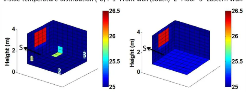
On the 12thJuly (15h UTC) we observe the inside temperature distribution for the two models
M1 and M2. Figure 3a/ shows that the sun patch touches some of the cells of wall 3 and 2. In Figure 3b/ the incoming radiation has been projected on all the cells of the floor. We can
observe that the floor cells’ are warmer than the other cells of the room. This last model
follows the traditional taken hypotheses by most of the simulation tools.
Figure 3: a/ with sun patch (M2) b/ incoming radiation projected on the floor (M1)
Despite the 25°C set point temperature, we notice differences on the temperature field (Figure 3) between both models. Maximal variations of 0.4°C are observed between the cells of the sun patch and the floor when comparing both models. This can explain the discrepancies between the two models when evaluating the power.
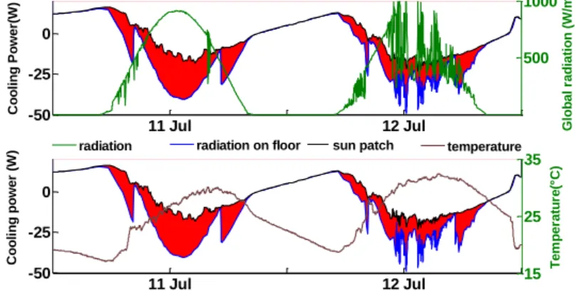
Cooling power is between 0 and 50W and gets more important when the temperature and the incident radiation is rises (Figure 4). Cooling power of M1 and M2 are compared. Discrepancies are observed, represented by the red area. Differences are larger when important solar fluctuations occur, during the day (red area). During this period the two models will project spatially the incoming radiation differently. With the sun patch model (M2) we have less cooling demand. For these two models and days of July, we have a relative difference of 83.9 %.
For the second case, we modelled the heating power necessary to maintain 20°C (Figure 5). Powers between 30 and 45 W are calculated. We observe discrepancies between these two
models only during the day time, as for the other configuration. With the sun patch model, more heating is required during the day. A relative difference of 3.6 % is obtained between these two models.
Figure 4: Cooling demand for M1 and M2
Figure 5: Heating power demand for a set point of 20°C for the two models
CONCLUSIONS
A 3D transient envelope model has been developed. In this model, we discretized the walls in small control volumes, with a refined meshing towards the surfaces. This spatial discretization enables to know where the sun patch is located at each time step. The weather data was sampled at a minute time-step, in order to take into account the fast climatic variations in time.
We applied this model to a low energy cell case, strongly insulated. A general similar trend between the results with the sun patch model and the results of S. Dautin [3] was found, knowing that we have a 3D model and in her work only 1D exchange were modeled. In the observed results of this paper, it seems important to consider the sun patch position for days with clear sky conditions. Higher discrepancies are observed between the two models for the cooling power demand than for the heating power demand. Taking too simplified hypotheses, like done with model M1, for clear sky conditions, could lead to important errors. These results were found for an important insulated cell but future studies for different configurations of cells will be realized in order to draw broaden conclusions on the impact of the sun patch on power demand.
These results have to be validated with experimental data, and therefore we are working on an in situ experimental set up.
11 Jul 12 Jul -50 -25 0 Cooling Power (W) C o o li n g P o w e r( W ) 500 1000 G lo b a l ra d ia ti o n ( W /m ²) 11 Jul 12 Jul -50 -25 0 C o o li n g p o w e r (W ) 15 25 35 T e m p e ra tu re (° C )
radiation radiation on floor sun patch temperature
3 Jan 4 Jan 30 40 50 H e a ti n g p o w e r (W ) 0 200 400 G lo b a l ra d ia ti o n ( W /m ²) 3 Jan 4 Jan 30 40 50 H e a ti n g p o w e r (W ) -10 -5 0 5 T e m p e ra tu re ( °C )
REFERENCES
1. M. Wall, « Distribution of solar radiation in glazed spaces and adjacent buildings.
Acomparison of simulation programs », Energy and Buildings, vol. 26, no 2, p. 129–135,
1997.
2. P. Tittelein, « Environnements de simulation adaptés à l’étude du comportement
énergétique des bâtiments basse consommation », Thèse de Doctorat, Université de Savoie, 2008.
3. S. DAUTIN, « Réduction de modèles thermiques de bâtiments: amélioration des techniques par modélisation des sollicitations météorologiques », Thèse de Doctorat, Université de Provence, 1997.
4. Stratégie utilisation rationnelle de l’énergie, chapitre II : « Les bâtiments », Ademe, www2.ademe.fr
5. La pointe d’électricité en France, Dossier de Presse, 2009. www.negawatt.org
6. C. Weinmann, S. Pasche, F. Gass, J. Beck, et C. Grange, « Prévision et justification des
consommations d’électricité pour 3 catégories de bâtiment », Echallens, Suisse,
Weinmann-Energies SA et Ecost, Rapport annuel, 2008.
7. TRNSYS 16 documentation, ‘Volume 6: Multizone Building modeling with Type56 and
TRNBuild’
8. EnergyPlus, Energy Plus Engineering Reference, Lawrence Berkeley National Laboratory, 2009
9. CODYBA www.jnlog.com/codyba1.htm
10. G.P Mitalas, D.G. Stephenson, ‘Calculation of Heat Conduction Transfer Functions for
Multi-Layer Slabs’, ASHRAE Annual Meeting, Washington, D.C., August 22-25, 1971.
11. J. Savoyat, K. Johannes, J. Virgone, 2011. Integration of thick wall in TRNSYS simulation. ISES solar world congress, Kassel, Germany, 2011
12. C. Flory-Celini, ‘Modélisation et positionnement de solutions bioclimatiques dans le
bâtiment résidentiel existant’, Thèse de Doctorat, Université Claude Bernard Lyon 1,
2008
13. B. Delcroix, M. Kummert, A. Daoud, and M. Hiller, « Conduction Transfer Functions in TRNSYS multizone building model: Current implementation, limitations and possible improvements », Fifth National Conference of IBPSA-USA, Madison, Wisconsin, August 2012.
14. International Daylight Measurement Programme, Station de l’ENTPE de Vaulx-en-Velin,