Prediction of wind effects on buildings using computational methods : review of the state of the art

Publisher’s version / Version de l'éditeur:

Canadian Journal of Civil Engineering, 21, 5, pp. 805-822, 1994-10-01

READ THESE TERMS AND CONDITIONS CAREFULLY BEFORE USING THIS WEBSITE. https://nrc-publications.canada.ca/eng/copyright

Vous avez des questions? Nous pouvons vous aider. Pour communiquer directement avec un auteur, consultez la première page de la revue dans laquelle son article a été publié afin de trouver ses coordonnées. Si vous n’arrivez pas à les repérer, communiquez avec nous à PublicationsArchive-ArchivesPublications@nrc-cnrc.gc.ca.

Questions? Contact the NRC Publications Archive team at

PublicationsArchive-ArchivesPublications@nrc-cnrc.gc.ca. If you wish to email the authors directly, please see the first page of the publication for their contact information.

NRC Publications Archive

Archives des publications du CNRC

This publication could be one of several versions: author’s original, accepted manuscript or the publisher’s version. / La version de cette publication peut être l’une des suivantes : la version prépublication de l’auteur, la version acceptée du manuscrit ou la version de l’éditeur.

Access and use of this website and the material on it are subject to the Terms and Conditions set forth at

Prediction of wind effects on buildings using computational methods :

review of the state of the art

Baskaran, B. A.; Stathopoulos, T.

https://publications-cnrc.canada.ca/fra/droits

L’accès à ce site Web et l’utilisation de son contenu sont assujettis aux conditions présentées dans le site LISEZ CES CONDITIONS ATTENTIVEMENT AVANT D’UTILISER CE SITE WEB.

NRC Publications Record / Notice d'Archives des publications de CNRC:

https://nrc-publications.canada.ca/eng/view/object/?id=a7fb75f8-7c97-4815-9f83-8ab2b24aca6d https://publications-cnrc.canada.ca/fra/voir/objet/?id=a7fb75f8-7c97-4815-9f83-8ab2b24aca6d

I

ER

'H

1

21d

1,2

LDG

. o .

3996

994

National Research Conseil national

1+1

Council Canada de recherches Canada

Institute for Institut de Research in recherche en Construction construction

Prediction of Wind Effects on

Buildings Using Computational

Methods Review of the State

of the Art

by A. Baskaran and

T. Stathopoulos

Reprinted from:

Canadian Journal of Civil Engineering

Vol. 21, pp. 805-822, 1994

(IRC Paper No. P-3996)

NRCC 3871 5

CISTI/ICIST NRC/CNRC

IRC Ser

Received on:

12-06-94

IRC paper

IRC paper

Prediction of wind effects on buildings using computational methods

-

review of

the state of the art'

A. BASKARAN

Institute for Research in Construction, National Research Council of Canada, Montreal Road, Ottawa, ON K I A OR6, Canada

A N D

T. STATHOPOULOS

Centre .for Building Studies, Concordia University, 1455 de Maisonneuve Boulevard West, Montreal, QC H3G IM8, Canada

Received June 26, 1992

Revised manuscript accepted February 7, 1994

Advancements in computer software and hardware technology provide a new direction for analyzing engineering problems. Recently the field of wind engineering has gained significant momentum in the computer modelling process. This paper reviews the state of the art in computational wind engineering, including the finite element method, finite difference method, and control volume technique. A portion of this paper summarizes the research in this area carried out by the authors. Computations have been made for a variety of building configurations, including normal wind flow conditions for a building with different aspect ratios, and modelling wind environmental conditions around groups of buildings. The computer modelling technique may eventually enhance the design of buildings and structures against wind loading and supplement the current design practice of using building codes and standards or performing experiments in wind tunnels.

Key words: buildings, computer modelling, pressure, velocity, wind engineering, wind tunnels.

Des progrks importants dans le dkveloppement des ordinateurs et des logiciels de modClisation ont Cte observCs dans le domaine de I'aCrodynamique et permettent de donner une nouvelle orientation a I'analyse des problkmes tech- niques. Cet article examine I'Ctat actuel de la technologie informatique dans ce domaine, y compris la mCthode des Clements finis, la methode des diffkrences finies et la technique du volume de contrble. Une partie de cet article rCsume la recherche effectuCe dans ce domaine par les auteurs. Des calculs ont CtC effectuks pour une variCtC de con- figurations de biitiment, y compris des conditions normales d'Ccoulement du vent pour un biitiment ayant divers rapports de forme, et une modClisation des conditions environnementales autour de groupes de bgtiments a Cte rCa- IisCe. La technique de modClisation informatique permettra eventuellement d'amCliorer la conception des biitiments et des structures en ce qui concerne les surcharges dues au vent. Elle constitue un complCment aux exigences con- tenues dans les codes et les normes du biitiment et aux essais en soufflerie.

Mots cle's : b2timents, modClisation informatique, pression, vitesse, akrodynamique, souffleries.

[Traduit par la rCdaction]

Can J Civ. Eng. 21. 805-822 (1994)

1. Introduction buildings with unique geometries or structural properties. buildings become tall and complex, i t becomes imper- Wind-tunnel studies on the Commerce Court Building and the ative to account for wind loads. Wind not only affects the CN Tower are

load distribution pattern on buildings but also influences In this paper, previous and current mathematical modelling various design parameters, w i n d effects on buildings are of turbulent, as well as steady, wind flow conditions around grouped in Fig. 1 under three major aspects; structural, envi- buildings are reviewed. Only a few studies have modelled ronmental, and energy. Some of the subcategories for each turbulent wind around buildings; they are presented in the stage is a l s o listed, is the of a building next section. However, significant efforts have been made in engineer to design safe and economical buildings by con- analyzing the variety of existing studies developed to predict sidering all these features. steady wind conditions (see Sect. 3). Attempts include appli- l n canada, building designers and engineers quantify these cation of the finite element method, the finite difference effects in accordance with the ~ ~~ ~ i l d i ~ ~ ~c o d e (NBC i ~ method, and the control volume method for wind engineering ~ ~ l

1990). i t s wind section has been derived mainly from the problems. The present review excludes many details of the results of sy sternatic ~l~~ note equations involved and the numerical formulation, in order that the ~ ~Building c o d e ~ iis one of the ~ ~ best ~ to emphasize the applications of the studies. These details can l documents available for the description of effects on be found in published dissertations, such as those of Vasilic- buildings. Engineering practice in Canada has extended to Melling (19771, Baetke (1986), Paterson (1986), and ~ a s k a r a n fabricating and testing scale models in wind tunnels for (1990). Section 4 provides a flavor of ongoing research by

presenting computations performed for a variety of building configurations. This includes computing normal flow con- Nore: Written discussion of this paper is welcomed and will be

received by the Editor u n t i l February 2X, 1995 (address inside ditions for a building with different aspect ratios, and mod-

front cover). elling wind environmental conditions around a group of 'part of this paper has been presented i n a variant form a t the buildings. Validation of the computed results has always Second Canadian Conference or1 Computing in Civil Engineering, been performed by comparison with the measured data from Ottawa, Ontario, August 5-7, 1992. different boundary layer wind tunnels. Finally, Sect. 5 reflects

C A N . J . CIV ENG. VOL 21, 1994

WIND

-b

Venfllatuon

I

1

F I G . I . Perspective of w~nd-induced effects on buildings (Baskaran 1990).

on the future of computerized approaches for the numerical evaluation of wind effects on buildings.

2. Computing turbulent wind flow conditions Computing the turbulent flow will provide the instantaneous pressures that are critical for the design of buildings claddings. Their prediction not only demands high computer resources but a l s o needs advanced numerical algorithms. Two approaches have been followed for the computation of tur- bulent wind flow conditions around buildings: the random vortex method and the large eddy simulation. In the former case, only time-dependent Navier-Stokes equations are con- sidered with constant fluid viscosity, whereas in the latter, the time-dependent form of the k-E turbulence model is also included. This section discusses the application of these methods for wind engineering problems; in-depth details of the methods can be found in review papers by Leonard (1980) for the vortex methods and Ferziger (1983) for large eddy simulations.

2.1. Random vortex method

T h e random vortex method f o r t h e solution of two- dimensional Navier-Stokes equations was first developed and presented by Chorin (1968, 1973, 1978). The incom- pressible flow of a slightly viscous fluid around a bluff body can often be characterized by three main flow regimes (Summers et al. 1985). Away from the body, the flow is largely irrotational and may thus be formulated in terms of potential flow theory. In the immediate neighborhood of solid surfaces, a boundary layer is formed in which the Prandtl boundary layer approximation is assumed to be valid. Beyond this boundary layer and in the downstream wake of the obstacle, the flow becomes complicated. This area has concentrated vorticity generated by the viscous interaction of the fluid with the obstacle.

Summers et al. (1985) applied the random vortex method to describe the viscous interaction of wind with surface- mounted obstacles of arbitrary cross sections. A logarithmic inlet velocity profile was selected to represent the stationary aspects of the atmospheric boundary layer. In Fig. 2, results from the random vortex method are illustrated for various building roof shapes. The buildings have the same eaves height (0.5 units) and width (1 unit), whereas the roof pitch angle varies (0, 23.5, 30, and 40 degrees). Figure 2 shows the streak lines formed by massless particles entering the flow as the first frame and followed over the successive time- steps, each step corresponding to 0.02 nondimensional time unit. The separation at the windward eaves moves to the ridge as pitch angle increases and reattachment can occur on the leeward roof side.

Bui and Oppenheim (1987) presented simulated results for air flow over a cube using the random vortex method. The two-dimensional computational flow domain is divided into two regions, one inside the boundary layer, where vortex sheets simulate the potential flow, and the other outside the boundary layer, where vortex bulbs develop in the flow. Mean wind velocity vectors are evaluated for a two-dimensional square model sitting inside a channel with a uniform approach velocity. Attempts were not made to compare these results with any measured data.

Along the lines of the random vortex method, the flow around bluff bodies can also be represented by the discrete vortex method. Inamerro and Saito (1985) used the discrete vortex method to study the unsteady flow around two- dimensional bodies having different aspect ratios. An extension of the discrete vortex method is also used by Inamerro and Saito for modelling the flows with various angles of attack; comparisons of the computed results with the experimental data show a significant difference when the wind angle is greater than 20 degrees. By applying the discrete vortex method, Bienkiewicz and Kutz (1989) computed Strouhal numbers for square and rectangular prisms and compared them with measured wind-tunnel data. The random vortex method has been improved over the years. One important improvement is the random sheet method presented by Chorin (1978). In this method the Prandtl boundary layer equation was utilized instead of the Navier-Stokes equation in order to eliminate singularity problems. Nevertheless, the nonrotating vortex sheets cannot be valid for turbulent boundary layer flows (Chorin 1986).

Recently, a fast vortex method for computing two-dimensional viscous flows has been presented by Baden and Puckett

( 1 990) and Turkiyyah and Reed (1993). These studies advance the state of the art of vortex methods by taking advantage of the evolution in computer hardware technology. For instance, the CPU time for the development of vector code is 10 times faster than conventional vortex methods. Ramsay (1991) also presented potential applications of rapid distortion theory in wind engineering. His approach involves the linearization of the governing equations, and it has been reported that the error due to neglecting the nonlinearity dynamics is small.

The random vortex method is advantageous for fluid flow problems because of its grid-free character. There is no need for an initial guess of the pressure field or flow separation points. Furthermore, the bluff body may have any arbitrary shape and its edges should not necessarily be sharp. However, the extension of this method to three-dimensional problems

BASKARAN A N D STATHOPOULOS 807

is not trivial. The other major drawback of this method is that it is not compatible with any standard turbulence models. This creates many difficulties in predicting the recirculation zones of the wind flow field. In any event, vortex methods have not been very attractive for wind engineering appli- cations, at least so far, because of the complexities in predict- ing high Reynolds number flows and other problems, as previously mentioned. Further discussion on these matters is found in Baetke (1986), Chorin (1980, 1986), Hanson et al. (1986), and Summers et al. (1986).

2 . 2 . Large eddy simulation

The large eddy simulation solves the Navier-Stokes equa- tion in time-dependent form and yields the fluctuating motions of turbulence. It is also possible in the simulation to analyze the turbulence statistics of the flow field at any instant. In this methodology, the main assumption is that the largest eddies dominate the physics of the turbulent process. Ferziger (1979) presented the following differences between large and small eddies:

( 1 ) The large eddies interact strongly with the mean flow and the small eddies are created mainly by nonlinear inter- actions among the large eddies.

(2) Most of the transport of mass, momentum, and energy is due to the larger eddies. The small eddies dissipate fluc- tuations of these quantities but affect the mean properties only slightly.

(3) The structure of large eddies is very strongly dependent on the geometry and nature of the flow, whereas the small eddies are much more universal.

(4) Due to their dependence on the geometry, the larger eddies are highly anisotropy. The small eddies are much more nearly isotropic and therefore universal.

(5) The time scales of the large eddies approximate the

time scales of the mean flow. For flow past a body, the large eddy scale is approximately equal to the dimension of the body divided by the free stream velocity. The small eddies seem to be created and destroyed much more quickly. Murakami et al. (1987) applied the large eddy simulation in two steps to compute time-dependent wind flow conditions around buildings. First, the solution procedure dealt with the development of the boundary layer and then the effect of air flow around a cubic model was analyzed. The time- dependent Navier-Stokes equations were solved by using the marker-and-cell method. All spatial derivatives were approximated by the central difference scheme. To model the turbulence, the Reynolds stress components were replaced by the large eddy simulation, as explained in Ferziger (1979), along with two Smagorinsky constants whose values were given by Laurence (1987). The execution of the algorithm takes 5-10 h in a super computer HITAC 810-20 to predict the wind velocities and turbulence intensities around a cubic model, as well as the pressure field of the flow. This study demonstrates the capability of super computers to solve the c o m p l e x i t i e s of turbulent Navier-Stokes equations. Unfortunately, frequent access to super computers is not common for most designers.

Numerical modelling using the large eddy simulation can predict instantaneous wind-induced parameters, as demon- strated by Song and He (1993). Even though the incoming flow was normal to the building, both the entire flow fields around the building and the flow fields of only half of the building, due to symmetrical conditions, were modelled. Typical results are shown in Fig. 3 in terms of lift and drag coefficient fluctuations. Clearly, the fluctuations are larger when only half of the building was considered, as normally happens in the modelling of steady wind flow conditions in order to reduce the computer resource requirements.

CAN. J . C l V . ENG. VOL. 21. 1994

0 20 40 60 80 100 120 0 20 40 60 80 100 120

Time Time

FIG. 3. Computed fluctuating lift and drag coefficients (Song and He 1993).

'

FENCE

_-L

_GROUND

'

SEPARATION BUBBLE (CAVITY)

= typical element

FIG. 4. Two-dimensional finite element arrangement around a fence (Street and Kot 1980). However, considering the Song and He findings, the assump-

tion of symmetry for spatial variation would be questionable for the simulation of time-dependent wind flow conditions. Thus time-dependent wind simulation will significantly increase the computer resource requirement.

3. Computing steady wind flow conditions

3.1. Finite element method

The era of finite element methods has little affected com- putational wind engineering, compared to the major break- through it has made in the aeronautical engineering. Never- theless, finite element methods have been utilized in a few computational wind engineering studies. As a first step in developing a three-dimensional finite element code for tur- bulent separating flows, Street and Kot (1980) presented a surface separation algorithm which takes the corner node of a three-dimensional bluff body immersed in turbulent flow and determines all the midpoints. Once the node location is established on the building, the optimum finite element mesh distribution around the building is formulated. The boundary conditions are imposed through a "stiffness" matrix, and the Gaussian elimination method is used for back sub- stitution of the solution vector.

Figure 4 shows a vertical section of this mesh distribution over a two-dimensional fence immersed in a turbulent bound- ary layer. Another interesting feature of this algorithm is the optimization process of the flow conditions. As the flow

evolves from the initial configuration, the elements lying on the separation surface move along with it and the other elements are then properly adjusted, based on the new sep- aration location. Yu and He (1985) attempted to compute the wind effects on a tall building using the finite element method. Triangular elements were used and pressure and velocities were computed using the same interpolating func- tions. The two-dimensional algorithm was found stable for various mesh arrangements and the equations were solved through the weighted residual methods of Baker (1983).

Uemura and Saito (1993) developed an automatic mesh generation algorithm to account for complex building con- figurations. A typical three-dimensional hexahedral mesh distribution is shown in Fig. 5. It is clear that the finite ele- ment method can accommodate more complex building shapes and orientations than the conventional finite difference formulation. Nevertheless, the freedom in applying the var- ious numerical schemes, such as HDS and SIMPLE (Patankar 1980), is restricted. Furthermore, the extension of the finite element method into three-dimensional problems is still in the research stage and needs significant refinement before it can be applied to wind engineering problems (Habashi and Peters 1987).

3.2. Finite difference method

The finite difference method is used in most studies for the computation of wind flow conditions around buildings.

B A S K A R A N A N D STATHOPOULOS

FIG. 5 . Three-dimensional finite element arrangement around a building complex (Uemura and Saito 1993).

W/W- Experiment 0 0 5 1 0

-

m Predlctions W/W_ Experiment 0 0 5 1 0

-

Pred~ctions m -4 -2 0 2 4 6 21 h

FIG. 6 . Comparison of the measured velocity profiles with the predicted data (Vasilic-Melling 1977).

Computational wind engineering continues to enjoy the ben- efits of finite difference techniques and this trend will prob- ably continue mainly because of two reasons: first, the finite difference method contains a wealth of established solution algorithms and numerical schemes that can be directly imported to computational wind engineering; second, these methods have the flexibility of accommodating turbulence models and time-dependent forms of the flow characteristics that are vitally important for the simulation of wind flow conditions. In finite difference method, wind flow problems can be simplified into flow over two-dimensional or three- dimensional bluff bodies; these problems are reviewed in the following subsections.

3.2.1. Two-dimensional works

One of the early attempts in numerical modelling of tur- bulent flow over bluff bodies was made by Vasilic-Melling (1977). Two-dimensional problems were considered first, to gain familiarity with the numerical solution procedure. Velocity and pressure predictions include ( 1 ) an infinitely

wide obstruction mounted to a free stream flow, (2) a wall-

mounted thin fence, and (3) a freely suspended thin fence in a uniform flow. For case (2), comparisons of the computed predictions with the available experimental data are shown in Fig. 6. The velocity profiles show large differences between the predicted and measured values within the shear layer and the recirculation zone. Underestimation of the acceleration

of the flow resulting from a block effect is also shown. Part of the discrepancies between the results near the wall may be caused by experimental errors. In particular, the measured

profiles in the recirculating flow, say d h = 2, show a trend

to an increasing reverse velocity near the wall rather than a tendency towards zero velocity, which is expected for a condition of no slip at the wall. Benodekar et al. (1985) also used the Vasillic-Melling methodology to predict the flow over surface-mounted ribs.

Hanson et al. (1984) investigated the possibilities of devel- oping a numerical model for wind flow problems around buildings. Their attempts included both the random vortex method and the control volume method for two-dimensional laminar flow of wind without adding the effect of turbulence intensity. The control volume method used originated from Caretto et al. (1972). Both methods were applied only to buildings with a symmetrical roof of arbitrary pitch. Attempts have not been made to compare the results with other studies or with the experimental data. However, the approach of this study brings out the advantages of the control volume method over the random vortex method.

Yeung and Kot (1985) computed turbulent flow over arbi- trary two-dimensional surface mounted obstructions by using the body-fitted coordinate system. One of the main appli- cations of body-fitted coordinate grid arrangement is mod- elling arbitrary geometrical configurations such as triangular and semicircular obstructions. The body-fitted coordinate

810 CAN. J . CIV. ENG. VOL. 21. 1994

-1.5

L

1 J

-

Paterson (1 990)

- - - Vasilic

-

~ e l l i n ~ ' ( 1 9 7 7 )

x x x x Catsro and Robins (1 977)

FIG. 7 . Comparison of the measured pressure coefficients with the predicted data (Paterson 1990).

grid systems are generated using the method of Thompson (1980, 1986), and in this process, one coordinate line will align with the solid geometry. The two-dimensional form of the k-E turbulence model is solved in closed form through the upwind difference scheme. Elliptical equations are obtained by transforming the Navier-Stokes equation into the vorticity-stream function form and solved by using the point successive over relaxation method. The computed reat- tachment length is found to be smaller in comparison with the experimental data of Counihan and Hunt (1974) and Woo et al. (1977). Attempts have also been made to improve the reattachment length by changing the values of the "universal constants" in the k-E turbulence models. Moreover, the artificial viscosity error introduced by the upwind dif- ference scheme was noticed and discussed.

Matthews (1985) attempted to compute the wind-induced pressure coefficients on a single building. A two-dimensional grid arrangement was utilized, and empirical values were used for the length scale and the intensity of turbulence. Mean pressure coefficients were computed for two buildings having different geometries. The velocity of the approaching flow was assumed to be uniform with height and normal to the predominant building dimension. The turbulence constants which had been proposed for the atmospheric boundary layer by Yeung and Kot (1985) were also used by Mathews (1987) and Mathews et al. (1988) for the computation of pressure coefficients on a semicircular greenhouse. The dependence of the pressure coefficients on the Reynolds number and on the exposure factor was evaluated. It was reported that the pressure coefficients are independent of Reynolds number greater than 3000. computations were performed for dif- ferent inlet boundary layer profiles; only a small variation was noted on the computed pressure coefficients.

Djilali (1987) used the TEACH code (Gosman and Pun

1974) to predict separated reattaching flow around a two- dimensional bluff rectangular section. For the laminar flow computations, two numerical schemes, namely the hybrid difference scheme and the bound skew hybrid difference scheme, are used. The results computed with the bound skew hybrid difference scheme agree better with the exper- imental data. S o it was decided to used the bound skew

hybrid difference scheme for the turbulent flow computations with the standard k-E turbulence models. However, the com- puted results underestimate the reattachment length by about

30%. The curvature correction of Leschziner and Rodi (1981) was applied to the turbulence models; as a result, the reattach- ment length, the kinetic energy, and the pressure field improved substantially. Durao et al. (1987) also noticed dis- crepancies between the computed and measured results when computing the two-dimensional flow around a square cross- sectional building by using the standard turbulence models with their universal constants.

Selvam (1989) performed two-dimensional computations using the stream function and vorticity method. Parameters

of two full-scale studies - Jensen and Frank (1965) on

Albertslud house and Marshall (1977) on a mobile home -

were input to the model and the computed results were com- pared with those from the wind tunnel, as well as with the full-scale data. The pressures from the computer modelling were reasonably close to the measured data, except for the leeward wall. Imposing better boundary treatment as opposed to the wall functions and identifying a suitable method for predicting the pressure field were suggested for improvements.

3.2.2. Three-dimensional works

Vasilic-Melling (1977) extended the procedure for three-

dimensional flows on surface-mounted cubes. A sensitivity

analysis of the numerical solution was made using a uniform upstream velocity profile. Experiments on flow visualization and velocity measurements were also undertaken. Compari- sons of the computed results were then made with the mea- sured data for mean pressures only. The study concluded that the numerical simulation did not faithfully represent the shear layer and recirculating flow which develops on

the downstream side of the obstacle. A better treatment of the

turbulence model parameters and the use of more suitable, instead of one-dimensional, wall functions have been sug- gested for future work. The significance of the study by Vasilic-Melling lies in the formation of a basic solution algorithm which has been subsequently modified on several occasions in order to solve the complicated nature of the interaction between wind flow and building.

BASKARAN A N D STATHOPOULOS Results of three-dimensional simulations of wind flow

around buildings were reported by Hanson et al. (1986). The discretized nonlinear equations of each cell was solved using a tridiagonal matrix algorithm with a successive over- relaxation factor of 1.5. No direct attempts were made to include the effects of turbulence. However, the viscosity of the incoming flow was increased by using an effective term in the numerical modelling. Since the study was concerned with the reverse-vortex flow which could aevelop between parallel buildings, only wind velocities were computed and compared with another study (Borges and Saraiva 1979) which measured the reverse wind velocity using sand erosion techniques. The wind speed ratios computed was also com- pared with the result of a wind-tunnel study (Penwarden and Wise 1973). From the comparison it was noted that the

deficiency of the simulation - its failure to reproduce the

compactness of the wake - could be improved by a more

detailed treatment of the turbulence. Semi-empirical turbu- lence models such as the k-E model have been suggested for further work in this area.

As a step toward validating the results obtained from mathematical models, Summers et al. (1986) used the wind tunnel data of Everett and Lawson (1984). From the various comparisons, it is clear that better computational tools are needed for the evaluation of wind effects around building configurations. Furthermore, the velocities computed at greater heights from the ground level agreed better than those computed at lower levels with respect to measured velocity values. This indicates that computational methods may provide better results for wind effects on tall buildings than on low buildings, which-are sitting at a greater distortion of turbulence. Wind tunnels encounter similar difficulties in the measurement of wind effects on low buildings.

By averaging the Navier-Stokes equation with respect to time, one can obtain the Reynolds equations. Paterson (1986) made a successful attempt at solving the Reynolds equations. T h e effect of turbulence in the flow was conveniently accounted for by means of the standard k-E turbulence mod- els developed by Launder and Spalding (1972, 1974). The control volume method was employed to discretize the non- linear partial differential equations. Algebraic equations were derived using the hybrid difference scheme. The alter- native direction implicit method was applied for the solution

of the resulting linear algebraic equations, and the SIMPLE

algorithm of Patankar and Spalding (1972) was used to ful- fill the condition of continuity. The computed results were compared extensively with three sets of wind-tunnel exper- imental data (Castro and Robins 1977, Woo et al. 1977, and Davies et al. 1979), as well as with two full-scale mea- surement results (Joubert et al. 1967 and Melbourne and Joubert 197 1).

All computations and comparisons were made for a single building, square or rectangular in plan form, placed in a continuous flow stream. The approach flow was always maintained normal to the obstacle, which brings the advantape of symmetry along the main axis for computational mc elling. Due to the discretization of the Reynolds equatior

only mean pressures were computed and compared with tl .

measured data. An example is shown in Fig. 7, which com- pares the computed pressure coefficients with the measured data of Castro and Robins (1977). Overall, the computed results agreed with the measured data. Note that an additional

term (C,,) as the reference pressure coefficient was given

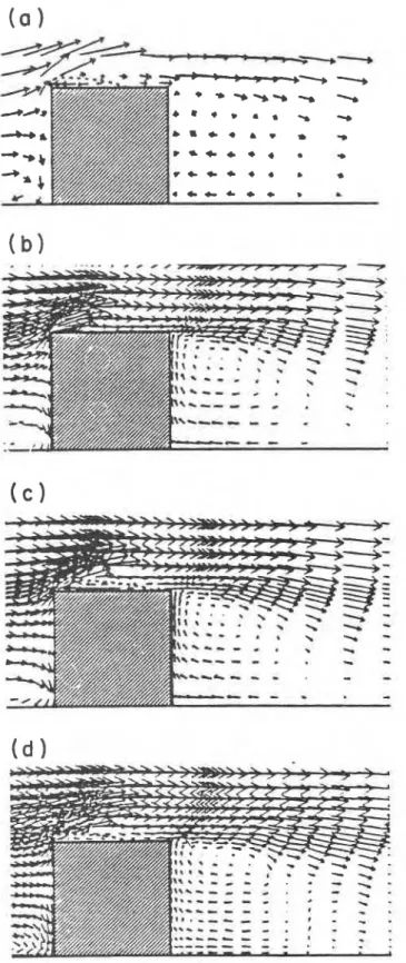
FIG. 8. Computed velocity field with different turbulence models:

( a ) wind-tunnel experiment; (b) k-E model; ( c ) algebraic stress

model; (d) large eddy simulation (Murakami 1993).

.. value of 0.07 to match the experimental data. For some cases, Paterson noticed neither the recirculation zone nor the pressure on the sides of the buildings seemed to be acceptable in comparison with the wind-tunnel data or full-scale values. Even for such simple cases like single objects with a normal incidence of wind flow, the computed parameters

CAN. J. CIV. ENG. VOL. 21, 1994 0 Summers et al. (1986) 8 Baskaran and Stathopoulos (1 989)

-

Probe

7

0 Summers et a!. (1986)

-

measured

2.

1

;;iA; (l;compute;

1

,

Baskaran and Stathowulos (1989)

0

0 100 200 300 400 0 100 200 300

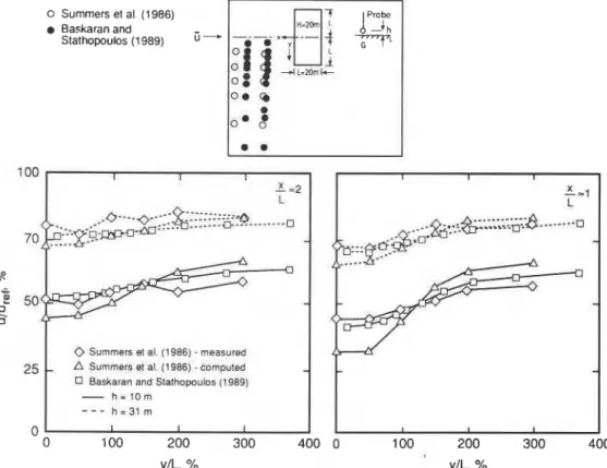
FIG. 9. Comparison of the upstream velocities with and without turbulence models (Baskaran and Stathopoulos 1989).

need improvements, particularly at the separation of the flow and in the wake.

Wind flow conditions around a cube have been studied by Baetke (1986) on a super computer in order to evaluate

the efficiency of vector codes. It was found that the CRAY

machine requires only 1/10 of the computing time in com-

parison to the scalar computer CDC CYBER 1 7 5 . The code

developed can run on any machine with architecture similar

to that of the CRAY. An elementary cubic-shape building

was used and extensive efforts were made in predicting the wind-induced pressure values for various grid arrangements. The quadratic upstream interpolation scheme of Leonard (1979) was utilized for the numerical discretization of the momentum equations. Comparisons of the computed results with the experimental data reveal significant differences for turbulent inflow conditions (Baetke et al. 1987). Inclusion of a better alternative method than the wall function approach is recommended to predict the wall shear stress at boundaries of separating and recirculating flow regions.

By using the standard k-E turbulence model, Murakami and Mochida (1988, 1989) computed the steady wind con- ditions around a cubic model. The standard wall functions of Launder and Spalding (1974) were used to bridge the bound- ary cell with the outer domain for all variables. To study the influence of boundary conditions on the numerical solu- tion, a constant pressure field and a zero pressure field were specified and only small differences were noticed on the computed results. Mesh resolutions around the windward and leeward corners were studied. Murakami (1993) also computed the wind flow conditions by applying three dif- ferent turbulence models, namely, the standard k-E turbulence model, the algebraic stress model, and the large eddy sim- ulation. Computed mean flow fields were compared with

the experimental data from the wind tunnel. Figure 8 shows

the vertical planes of the vector plots. In general, all three tur- bulence models produced similar mean wind flow conditions around the building.

4. Current research efforts

Current research efforts into the computer modelling of wind effects on buildings can be summarized into three parts: computations with conventional turbulence modelling (Sect. 4.1), computations with improved turbulence modelling (Sect. 4.2), a n d computations using microcomputers (Sect. 4.3). Both the momentum and continuity equations are solved together with semi-empirical turbulence models in three-dimensional form. The control volume method is used for discretization and the hybrid difference scheme is applied for the convective term interpolation. The linearized algebraic equations are solved using the alternative direction

implicit method and the SIMPLE algorithm finds the unknown

pressure field in a staggered grid arrangement. To perform the computations efficiently, a new modular structure com-

puter code named TWIST - Turbulent Wind Simulation Tech-

nique - has been developed. Details of the coding and

methodologies can be found in Baskaran (1990).

4 . 1 . Computation with conventional turbulence modelling This section examines the importance of turbulence mod- elling in the computation of wind effects around buildings. This has been conveniently demonstrated by analyzing two computed cases: one without including any turbulence model and the other by incorporating the k-E turbulence model. Both computed results are compared with the measured data from the boundary layer wind tunnel. In addition, this section examines the capabilities of the standard k-E turbulence model and the conventional wall function approach for the boundary treatment in modelling wind environmental con- ditions around buildings.

BASKARAN AND STATHOPOULOS 0 Summers et al. (1986) Baskaran and Stathopoulos (1 989) ii -+ Probe 9 0.

.

0 0

.

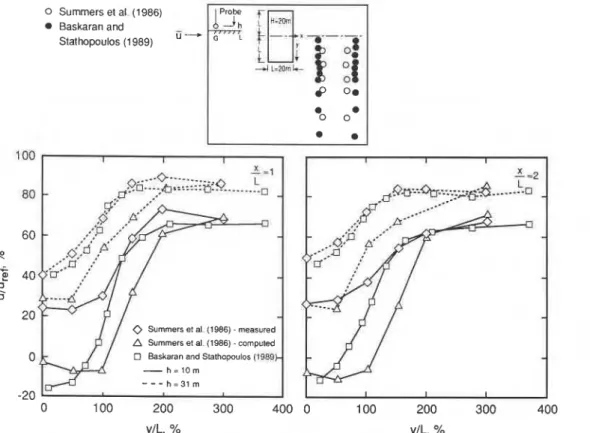
0 Summers et al (1986) -measured

A Summers el al. (1986) -computed Baskaran and Stathopoulos (1989b

-

h = l O m

0 100 200 300 400 0 100 200 300 400

y/L, % y/L, %

FIG. 10. Comparison of the downstream velocities with and without turbulence models (Baskaran and Stathopoulos 1989).

CAN. 1. CIV. ENG. VOL. 21, 1994 SIDE VIEW Z h 8 2 x 4.5 I

I I

I I 1 1 1 1 1

il

~ ~ i ~ l ~ ~ l l l i ~

!

: ~ i l ~ l l i I I I I I I I

I

!

I I

! : h PLAN VIEW Y l 8 2 x 6 e I

8

' I _{, -} 11(11 ,.-..

:

2.88

-

, 1 '

-

1 1 :

-

/ , I . 8 ' ., Ill, . _, 3 , I I I I . , : / Ill .I . I1 I . , 1 , I I

-

FIG. 12. Plan and side view of the computational grid (Stathopoulos and Baskaran 1 9 9 0 ~ ) .

Figure 9 presents the time-averaged longitudinal velocity component, u. Data are presented as percentages of velocity ratios referenced to free stream values of a particular location and they are compared for a number of points, at two loca- tions at the building upstream, for flow normal to the building face. Because of symmetry, both measurements and com- putations were made only for half of the flow domain, at two heights of approximately

5

and 16 cm, representing 10 and 31 m, respectively, in full scale. Three curves on each set represent the computed values of the present study; the com- puted values of Summers et al. (1986); and the wind-tunnel data, also reported by them. Baskaran and Stathopoulos (1989) included the standard turbulence model during the computation, whereas the computed values of Summers et al. (1986) were generated without considering turbulence. The measured data are obtained from a boundary layer wind tunnel. The incident wind was modelled by the power law form with the exponent equal to 0.21 and the reference height equal to 38 cm. The building block had the following dimension ratios: width:length:height = 4:2:3. Further details of the measurements are provided in Everett and Lawson (1984).

From the comparisons it is clear that the computational

tools can predict the overall nature of the flow conditions. However, deviations from the wind-tunnel values smaller than those of Summers et al. (1986) were noted by Baskaran and Stathopoulos (1989). A similar feature appears in Fig. 10, which shows the comparisons for two downstream locations in the same format as in Fig. 9. Poor agreement of both sets of computational values is evident near the building. For the downstream side, when the measurement height is 10 m from the ground level, the numerical simulations deter- mine negative values, i.e., a revese flow is calculated, whereas the wind-tunnel measurements show at these locations a positive (i.e., streamwise) flow. However, the values obtained in the present study are generally closer to the wind-tunnel data. As shown in the figure, the solution grids are slightly different and did not exactly correspond in the two studies, but this makes little difference in these com- parisons. The pertinent question of Summers et al. (1986): "Whether the most obvious deficiency of the simulation -

its failure to reproduce the compactness of the wake -

could be improved by the introduction of a more detailed treatment of turbulence," is considered in Baskaran and Stathopoulos (1989) by incorporated the well-known k-E

BASKARAN AND STATHOPOULOS

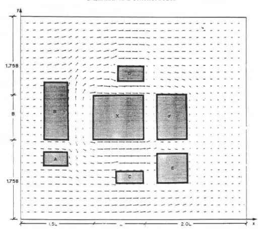
FIG. 13. Vector plots of the computed velocity field around the buildings (Stathopoulos and Baskaran 1990a).

results with the experimental data is attributed to this addi- Scale

tional mathematical treatment of the flow.

(2)

0 I u 2

The feasibility of evaluating wind environmental conditions

around multiple building configurations has also been exam- - Measured

- - - -

ined (Stathopoulos and Baskaran 1 9 9 0 ~ ) . In this study, an Computed

attempt has been made to simulate the wind environmental conditions around an actual downtown location in Montreal.

The cluster of buildings A, B, C, D, E, and F around the

Concordia University Hall building, X, is shown in Fig. 11.

These are the major buildings in the so-called proximity region, which have been modelled for the numerical com- putation as well as for the experimental measurements. These buildings have been assumed to have rectangular cross sections. Approximate dimensions of all these buildings and the exact locations of the points of measurements of wind speeds are also shown in the figure. The selected points are at the sidewalks or corners of the building under con- sideration to monitor the local wind characteristics.

A computational grid mapping of the domain is shown in Fig. 12, which displays the relative building location. Both the plan view and the side view of the buildings are shown. In the plan view, there are 82 nodes along the wind direction and 69 nodes along the lateral direction. There are 48 nodes in the vertical direction. The size of the com- putational domain in each direction is also shown. The grid distribution is denser in the proximity region and the arrange- ment contains in total 267 648 nodes. From the figure, it is also clear that the assumption of symmetrical conditions is not valid, even for the normal (SW) wind flow conditions. This makes the size of the computational domain different from the study of wind flow around a single building. More- over, available computer resources do not permit any increase in the number of nodes. On the other hand, attempts to

reduce the number of nodes to 52 X 55 X 42 led to diver-

FIG. 14. Comparisons of the computed and measured velocity

ratios at 2 m from the ground level (Stathopoulos and Baskaran 1 9 9 0 ~ ) .

gence of the computational algorithm. This is because with the reduction of the number of nodes the grid spacing increases and this creates larger discontinuities of the cal- culated variables, which in turn causes divergence in the computation.

I I I I wlndward wall ,

-

-

-

MeasuRd Computed I I I I

CAN. J. CIV. ENG. VOL. 21, 1994 100

CP -Cp

F I G . 15. Comparison of the measured pressure coefficients with the predicted data (Baskaran 1990).

FIG. 16. Comparison of the streamline plots around a building (Baskaran 1990).

Figure 13 shows the plan view of the computed velocity

fields around the buildings at 2 m from the ground level.

This two-dimensional velocity plot takes into consideration the longitudinal, u, and lateral, v, components of the velocity vectors. Flow separation points, changes in wind directions

along the two sides of the Hall building, X, and wake regions

are clearly shown in the figure. The velocity components are smaller in the recirculation area and also at the centre of the building front. The changes in the wind flow direction around the surrounding buildings are also clearly indicated. Vector plots, such as those of Fig. 13, are useful as pre- liminary information for the designer, architect or engineer. Quick derivation by the computer and flexibility in incor-

poration of changes are sufficiently impressive to stimulate enthusiasm about computer evaluation of wind effects on buildings as opposed to the traditional wind tunnel modelling approach.

To evaluate the changes in the local wind environmental conditions, the calculated velocities are converted into con- ventional velocity ratios. These ratios are obtained by dividing the magnitude of the velocities around the building under consideration by the velocities in the absence of the building. Since the velocities are taken at the same height for a partic- ular location, these ratios will directly indicate the influence of the building under consideration on the local wind con- ditions. Values greater than unity indicate an increase in

BASKARAN AND STATHOPOULOS 817

considered accurate in these locations.

Comparisons between the computed and measured pressures on the building envelope have also been made to establish the adequacy of the computational approach. Pressures are con- verted into the conventional form of nondimensional pressure coefficients normalized with the dynamic pressure at the building roof height. Figure 15 shows typical comparisons for the walls. The coefficients are plotted against the ratios of

?/H, where

z

is the height of the pressure tap or the grid location measured from the ground level and H is the height of the building. Experimental values provided in Stathopoulos and Dumitrescu-Brulotte (1990) are used as the measured wind-tunnel data. These data originate from the model of a 55 m high building tested in a turbulent boundary layer wind tunnel. Measurements from normal wind flow conditions are considered for the comparisons. Overall the computed pressure coefficients agree well with the measured values. There is little difference between the measured and computed values for the front and leeward walls. However, deviations are more significant when computed negative values are compared with suctions measured on the sidewall, particularly near the bottom and the top of the wall. This discrepancy is attributed to the standard turbulence model, which may not be representative of the streamline curvature of the flow.

the velocity due to the presence of the buildings. On the 1 .00

other hand, ratios less than 1 indicate a reduction of local velocity when the building is added. These ratios can be

further used to evaluate pedestrian comfort around building 0.75

X and to examine the impact of the construction of building

X, if this is a proposed building, on the wind environmental

_c~

conditions in the area. The velocity ratios (amplification or 0.50

reduction factors) are compared in Fig. 14 for the multiple building configuration. Magnitudes of the ratios are higher

at the building corners in comparison to the other locations. _0.25

The results show generally good agreement (within 30% discrepancy) with the exception of two points. Both these points are in highly complex recirculating flow regions.

0

Consequently, neither measured nor computed values are

4.2. Computation with improved turbulence modelling The previous section refers to computations made using the

I I I I I

-

-

-

Wlnd I I 4 I I I I I I

standard k-E model to mimic the iurbulence in the flow.

The conventional wall functions have been used as boundary conditions for all variables involved in the computation. Comparisons of the computed results with respective wind- tunnel data have revealed the following:

(1) considered mathematical equations and boundary specifi- cations can predict overall flow features around buildings;

(2) computed velocity fields at the downstream of the flow

and the length of recirculation zones behind the building

_,

are significantly underestimated;

ROOF

-

-

I

,

:

:

.

:

-:

:

Experiment A Zonal Treatment Wall Functions

i

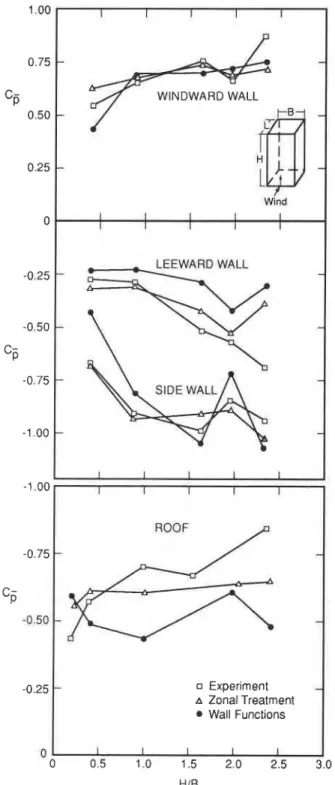
HIB

FIG. 17. Computed and measured averaged pressure coefficients

3n the building envelopes (Baskaran 1990). (3) induced suction values on the building envelope have

not been computed accurately, particularly on building sidewalls where usually the flow is complex.

Validity of the standard k-E turbulence model and its con-

stants is questionable for recirculating and separating flows (Rodi 1975; Hanjalic and Launder 1979, 1980; Rodi and Scheuerer 1986; Bernard 1986). The calculated turbulent shear stress is insensitive to the streamline curvature of the flow and hence the turbulent viscosity is not affected by the local flow behavior. In addition, only a low rate of dis- sipation of turbulent kinetic energy is computed when stan-

dard k - ~ turbulence models are used. To account for these

effects and to improve the predictions, two simple modifi-

cations on the standard k-E turbulence models, namely

streamline curvature correction (Leszchziner and Rodi 1981) and preferential dissipation correction (Gibson 1978), have been identified and applied (Baskaran and Stathopoulos 1989). Specification of boundary conditions plays a major role in the numerical modelling process. Previous studies used the conventional wall functions to bridge the solid boundary control volumes with the outer cells. When wall functions are

applied for all variables of computation (u, v, w, k , E ) , the

near wall turbulence properties are underestimated. This is due to the fact that the wall functions are developed based on one-dimensional Couette flow assumptions (Van Der

. VOL. 21, 1994

8 18 CAN. J. CIV. ENG.

600

Number of nodes

FIG. 18. CPU time requirements with different computer systems (Baskaran and Stathopoulos 1992).

Berg 1975) and they are valid only for the velocity variables (Pate1 et al. 1985; Launder and Shima 1989). Thus for the turbulence variables (k and E), a new effective zonal treatment method has been developed, whereby the local Reynolds number is used to monitor the near wall flow region and expressions derived are based on the Taylor series expansion technique. Stathopoulos and Baskaran (1990b) reported that the results of this approach agree well with the measured data. Figure 16 displays the flow field by means of streamline plots by using the zonal treatment and the more traditional wall functions approved. A vertical section passing through the centre of the building is shown. Both approaches utilize the same optimum grid distribution and other input para- meters. The change in the flow path relative to the compu- tational domain is clearly shown in the figure. Recirculation and distribution of the eddies are predicted reasonably well by the new approach. Moreover, the upwind vortex at the windward side of the building is shown clearly for the zonal treatment method. Furthermore, experimental results from Stathopoulos and Dumitrescu-Brulotte (1990) and Baskaran (1986) have been used to compare wind-induced pressures. Several building configurations and exposure conditions have been considered. Computed and measured pressures have been transformed into nondimensional pressure coef- ficient forms referenced to the respective building roof height. From the pressure coefficients computed or measured, the maximum value that has been found on each horizontal wall section has been retained. The arithmetical mean of all these values provides an average critical pressure coef- ficient for each wall. Thus a single parameter (i.e., average pressure coefficient) for each wall is obtained by post- processing large amounts of available data in order to judge the general accuracy of the numerical predictions.

Figure 17 shows the comparisons of such average pressure coefficients for a square building with different H/B ratios. The results computed using the new zonal treatment method are mostly in good agreement with the measured data. Clearly, encouraging improvements are obtained for the building sidewall irrespective of the building height. The

suction values measured for the leeward wall increase as

H/B increases. In the computational approaches, this trend

breaks down for H/B > 2; at H/B = 2.4, a significant dif- ference can be noticed between the computed and measured values. This discrepancy may also be due to experimental uncertainties involved in the measurements, including dif- ferences between the location of pressure taps and compu- tational grid points. In general, the zonal treatment method is preferable in comparison with the wall function approach. Nevertheless, such comparisons also show the level of agree- ment that is currently achieved between the measured and computed results.

4.3. Computation using microcomputers

Computational speed and the storage capacity of micros are increasing day by day, as well as their usage by the engineer- ing community. To permit the use of this present research by professional engineers, a version of the computer code has been developed and implemented in various microcomputers. Two major problems were encountered during this process: storage capacity of the micros and floating point handling. The storage capacity of the micros limits the size of the independent ariay to 64K, and it reduces the total program memory size to about 565K. These restrictions will vary, depending on the memory left over after the system require- ments; the authors' computations took less than 540K DOS memory. However, to overcome the restriction of 64K, the compiler data threshold option was used along with huge memory model setting. Handling the floating point depends on the math co-processor of the respective micros. The tol- erance threshold values are suitably adjusted, depending on the micros.

The number of computer grid nodes plays a major role in the CPU time required for the numerical evaluation of wind effects on buildings. Keeping the extent of the com- putational domain constant, the number of control volumes inside the domain has been varied to establish the parameters for economical computation. Runs were made on different computer systems based on feasibility, i.e., capacity limits. Figure 18 presents the CPU time as a function of the number of grid nodes. The CPU time corresponding to microcom- puters represents the direct, continuous access time. The VAX machines operate with the unique page faulting and virtual memory address technology, and their CPU time is taken under batch mode operation. Microcomputers with longer word length and higher clock speed consume less CPU time, as expected. On the other hand, the hard disk access time does not affect the CPU time because of the iterative nature of the problem. Both IPCI12 and DELL 286120 have the same Intel 286 microprocessor but the high clock speed DELL takes less CPU time. It is also interesting to note that both DELL and AST have the same clock speed, but the AST with longer word length consumes less CPU time. Figure 18 also contains an empirical relation for the CPU time required to run under different computer systems. Baskaran and Stathopoulos (1992) concluded the following for the computation of wind effects on buildings in different computer systems:

(1) Microcomputers require a CPU time which is 9-36 times more than the time necessary for the same run in the VAX machines.

(2) Among the various computational parameters, the CPU time required for computation increases quasi-linearly with the number of grid nodes.

BASKARAN AND STATHOPOULOS 819 (3) Since the problem considered is iterative in nature, the

disk access time has only marginal influence on the total CPU time required for the solution. This was true of all three computer runs examined.

(4) Economical computations can be achieved using 32-bit machines with high clock speed.

5. Future outlook, directions, and concluding remarks

Numerical modelling of wind effects on buildings is a new technique under continuous development and can be used to complement the existing wind-tunnel experiments. None of these various computational methodologies presented in the paper have a wide range of practical applications and thus research continues unabated on all fronts. Identifying future directions in this research field is rather difficult. because of the major involvement of computer resources and their unpredictability, both in terms of hardware and software. This section simply provides a bird's eye view of some influences on the calculation of the complex wind flow conditions around buildings.

Very few attempts have been made in the calculation of unsteady turbulent wind flows in computational wind engi- neering. Need for extensive computing resources on one hand and lack of direct simulation schemes on the other seem to be the major constraints. Research efforts using high-level turbulence models (Murakami et al. 1987) and super computer facilities (Baetke 1986) faced problems of validating their computed results directly with experimental data. One way to overcome this problem is to concentrate on the probability distribution functions of the unsteady com- ponents, rather than on single individual peak values.. Wind- tunnel and full-scale studies also treated the time-dependent peaks in this fashion (Dalgliesh 1971; Peterka and Cermak

1975; Stathopoulos 1980).

When reviewing the computation of steady wind flow conditions, the following numerical procedure was found to be successfully for many building configurations: control volume method for the discretization of the nonlinear partial differential equations, SIMPLE algorithm to fulfill the flow continuity, and alternative direct implicit method to solve the linear algebraic equations. A staggered grid arrangement also goes along with this package to take advantage of the unknown pressure field. However, for buildings with different shapes, the body-fitted coordinate grid systems may be appropriate (Richards 1989). To address the geometrically complex buildings, further research is necessary. Using orthogonal grid strategies or converting the complex domains into definable domains using decomposing techniques or developing suitable boundary adjustment methods with the body-fitted coordinate systems are worth investigating.

The review of turbulence closure can be found in Spalding (1982), Rodi (1984), Markatos (1986), Hunt (1988), and Leschziner (1989). One feature that is clear from these stud- ies is that the engineering community continues to enjoy the

k-E

turbulence model or its variants. This attraction is due to the formulation of the

k-E

turbulence model using transport equations containing convection, dissipation, and source terms such that they can be compatible with the momentum equation in the solution procedure. This model can also pre- dict reasonable results for engineering applications at an affordable computational cost. The authors' experience, although limited, also reveals that the

k-E

model is generally more suitable for wind environmental applications than the

evaluation of the structural loads. Much research is needed to study the full capacity and limitations of the

k-E

equations or their variants for the computation of wind flow conditions. The application of other forms of turbulence closure, such as Reynold stress models, algebraic stress models, and other stress-flux models, is basically in the initial stage.

Another important tissue in the numerical modelling of wind effects on buildings is validating the computed results. This is considered an integral part of model development, since only systematically validated codes can earn the con- fidence of designers. Wind flow mechanisms are often com- plex, partly because the fundamental relationships are non- linear and partly because there are many physical processes involved. Therefore when developing the code, clear knowl- edge of the basic flow mechanisms for simplified conditions (e.g., a single building exposed to normal wind conditions) is necessary. Experimental data are always used to evaluate computational results, although this is disputable in some cases. Nevertheless, documenting and using well-scrutinized wind-tunnel data should exclude experimental errors and differences. For low buildings, the results from the Aylesbury comparative experimental program (Sill and Cook 1989) may be used, since a comparison with the field data is often desirable. The wind engineering research facility, a collab- orative program of Colorado State University and Texas Tech University supported by National Science Foundation, is also a unique resource for experimental data. For tall buildings, Dalgliesh and other members of the National Research Council Canada monitored the 57-story Commerce Court building during the period 1973-1980 and collected data that include wind-induced surface pressures. The com- putational wind engineering community can make use of these systematically collected data to validate their computer codes.

Computational fluid dynamics and its application to wind engineering are rapidly growing. In the-last two or three years several symposia and congresses have taken place adding new research findings to the state of the art. In North America, a task committee has been formed in 1991 under the auspices of the Aerodynamics Committee of the American Society of Civil Engineers (ASCE) and has organized several computational wind engineering conference sessions. The first computational wind engineering conference was held at the University of Tokyo (Murakami 1992). The conference had about 230 attendees from 20 countries, presenting 92 papers in 23 sessions. For the first time, experts from computational fluid dynamics were brought together with those from wind engineering to address the complexity in numerical modelling of wind effects on buildings. There were 12 invited lectures, 4 from U.S.A., 2 each from Japan, Canada, and United Kingdom, and 1 each from Germany and France. Furthermore, the 7th U.S. National Wind Engineering Conference also had several presentations on the application of computational fluid dynamics to the wind engineering field (Hart 1993).

It is clear that the computer modelling technique may eventually enhance the design process of buildings and structures against wind loading, ventilation, and other environ- mental conditions, including dispersion of pollutants. This will complement the current design practice of using building codes and standards or performing experiments in wind tun- nels. Experiments and computer modelling have to be carried out in parallel and to complement each other in identifying