Phoenix model measurement and bifilar swinging

(1)

Publisher’s version / Version de l'éditeur:

Vous avez des questions? Nous pouvons vous aider. Pour communiquer directement avec un auteur, consultez la première page de la revue dans laquelle son article a été publié afin de trouver ses coordonnées. Si vous n’arrivez pas à les repérer, communiquez avec nous à PublicationsArchive-ArchivesPublications@nrc-cnrc.gc.ca.

Questions? Contact the NRC Publications Archive team at

PublicationsArchive-ArchivesPublications@nrc-cnrc.gc.ca. If you wish to email the authors directly, please see the first page of the publication for their contact information.

https://publications-cnrc.canada.ca/fra/droits

L’accès à ce site Web et l’utilisation de son contenu sont assujettis aux conditions présentées dans le site LISEZ CES CONDITIONS ATTENTIVEMENT AVANT D’UTILISER CE SITE WEB.

Student Report (National Research Council of Canada. Institute for Ocean Technology); no. SR-2005-29, 2005

READ THESE TERMS AND CONDITIONS CAREFULLY BEFORE USING THIS WEBSITE.

https://nrc-publications.canada.ca/eng/copyright

NRC Publications Archive Record / Notice des Archives des publications du CNRC :

https://nrc-publications.canada.ca/eng/view/object/?id=a5dcdfbf-b6ca-411b-ae4d-7a210c10bec1 https://publications-cnrc.canada.ca/fra/voir/objet/?id=a5dcdfbf-b6ca-411b-ae4d-7a210c10bec1

Archives des publications du CNRC

For the publisher’s version, please access the DOI link below./ Pour consulter la version de l’éditeur, utilisez le lien DOI ci-dessous.

https://doi.org/10.4224/8894965

Access and use of this website and the material on it are subject to the Terms and Conditions set forth at Phoenix model measurement and bifilar swinging

(2)

REPORT NUMBER

SR-2005-29

NRC REPORT NUMBER DATE

December 14, 2005

REPORT SECURITY CLASSIFICATION DISTRIBUTION

TITLE

Phoenix Model Measurement and Bifilar Swinging AUTHOR(S)

G. Hewitt, E. Waterman

CORPORATE AUTHOR(S)/PERFORMING AGENCY(S)

PUBLICATION

SPONSORING AGENCY(S)

Institute for Ocean Technology

IOT PROJECT NUMBER

42_2117_10

NRC FILE NUMBER

KEY WORDS

Bifilar Swing, Phoenix Underwater Vehicle

PAGES 17 FIGS. 6 TABLES 4 SUMMARY

This report describes the methods used to measure and describe the Phoenix underwater vehicle model. This included measurements for mass, length, center of gravity, buoyant force, radius of gyration, and moment of inertia. The radius of gyration and moment of inertia values were calculated based on the period of oscillation found from bifilar swinging the model. An uncertainty analysis of the results is also presented here. The method and apparatus described in this report proved to be accurate to within ±2mm and could be repeated for other underwater vehicles in the future.

ADDRESS National Research Council

Institute for Ocean Technology Arctic Avenue, P. O. Box 12093 St. John's, NL A1B 3T5

(3)

Institute for Ocean Institut des technologies

Technology océaniques

PHOENIX MODEL MEASUREMENT AND BIFILAR SWINGING

SR-2005-29

Gerald Hewitt, Erin Waterman

(4)

Summary

In October 2005 a model of the Phoenix underwater vehicle was tested in the Ice Tank at the Institute for Ocean Technology (IOT). After these test were completed the vessel was reassembled in each of five configurations and its geometrical properties measured in the Autonomous Underwater Vehicle (AUV) Lab at IOT. The method used to measure these parameters and the results of those measurements are presented in this paper.

Measurements of the length and mass of each vehicle configuration were made. The buoyant force of each configuration was found by submerging each vehicle while it was hanging from two load cells. In this manner the load cells could also be used to locate the center of gravity (CG).

The yaw radius of gyration of each configuration was found using bifilar swinging. First the dry model was hung from two filaments and oscillated laterally about it’s CG. The period of oscillation was measured and used to calculate the radius of gyration. This procedure was then repeated with the model flooded, hanging in air to determine the radius of gyration of the flooded model. The results of these measurements are presented in this report.

To determine if the swing apparatus was affecting the measurements, a solid aluminum rod was swung from the apparatus as well. The radius of gyration calculated form this swinging was very close (±1 mm) to the theoretical calculated value for that rod. An uncertainty analysis of the results is also presented here. The uncertainty analysis, coupled with the results of swinging the aluminum bar, show that the methods and apparatus used here are valid within ±3 mm, and can be used for other vehicles in the future.

(5)

List of Figures

Figure 1 - The five different configurations of Phoenix ... 5

Figure 2 - Arrangement of Ring and Acrylic... 5

Figure 3 - Connection of two adjacent acrylic pieces... 6

Figure 4 - Dry Swing Apparatus... 8

Figure 5 - Close up View of Pinch Clamp... 8

Figure 6 - Apparatus for Wet Model Measurements ... 9

List of Equations

Equation 1 - Radius of Gyration from Period Measurement ... 4

Equation 2 - Moment of Inertia of a rod about its axis... 10

Equation 3 - Radius of Gyration - Theoretical... 11

Equation 4 - Radius of Gyration in terms of length... 11

Equation 5 - Radius of Gyration Uncertainty ... 14

Equation 6 - Partial Derivative of K with respect to T ... 14

Equation 7 - Partial Derivative of K with respect to D... 14

Equation 8 - Partial Derivative of K with respect to L ... 15

Equation 9 - Discrete Uncertainty Equation ... 15

List of Tables

Table 1 - Length and mass measurements for each configuration... 12

Table 2 - CG locations for each configuration... 12

Table 3 - Radius of Gyration for each configuration... 13

Table 4 - Moment of Inertia for each configuration ... 13

(7)

Background

In October 2005, tests were conducted in the Ice Tank using the Phoenix model. Five different configurations were used for this testing. Each configuration represented a different length-to-diameter ratio, ranging from 8 to 12. These tests consisted of several different maneuvers including arc-of-a-circle. Once the tests were completed the vehicle, and all the parts required for each configuration were brought to the AUV lab for

measurements and testing. This involved measuring the geometrical properties and mass of each component, weighing each configuration of the model in air and in water. It also included locating the center of gravity (CG) of each configuration dry, in water and flooded in air. The Moment of Inertia (MOI) for dry and flooded models was also required.

To determine the Moment of Inertia of each configuration, bifilar swinging was employed for each configuration. Bifilar swinging involves hanging the model horizontally from two vertical wires (filaments) equally spaced on either side of the center of gravity. The model is then offset, in yaw, from rest and the period of oscillation measured. In this case we measured the time for 10 oscillations and divided by 10 to get the average period. This was repeated five times for each configuration. Each of the five period measurements was used to calculate a radius of gyration and those radii averaged to get the final radius.

L g TD K 4 =

Equation 1 - Radius of Gyration from Period Measurement

Where:

K = Radius of gyration (m) T = Period of oscillation (s)

D = Distance between filaments (m) g = Gravitational constant (9.806 m/s2) L = Length of the filaments (m)

(8)

Configurations

The configurations for the Phoenix vehicle were constructed using the same nose, tail and center body sections. Each configuration then had the required number and length of acrylic pieces (A1, A2, A3, F1, F2, F3) added to make the appropriate length. For increased support, each of these acrylic pieces was supported from the inside using a stainless steel ring. The acrylic pieces were manufactured such that when each piece is assembled in configuration LD12 the labels of each component line up with each other and the labels of the steel rings are visible on the bottom of each piece, as shown in the figure below.

Figure 1 - The five different configurations of Phoenix

Figure 2 - Arrangement of Ring and Acrylic.

(9)

Figure 3 - Connection of two adjacent acrylic pieces

(10)

Apparatus

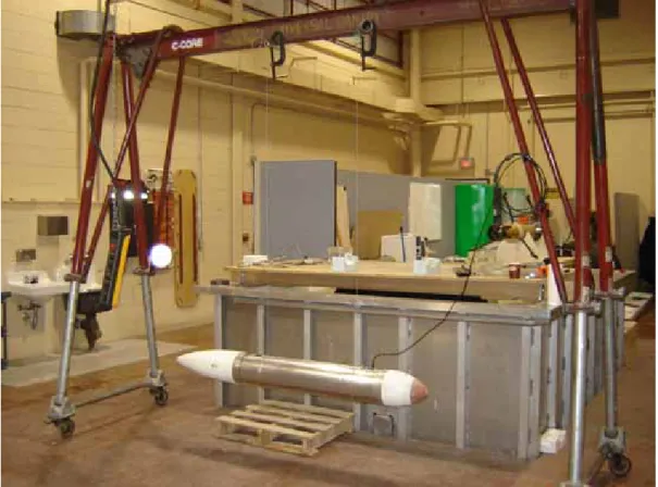
All the measurements required were taken at the Autonomous Underwater Vehicle (AUV) Lab at IOT or using the scales located in the Model Prep Shop. The test apparatus for bifilar swinging and in-water testing is shown below.

Figure 4 - Bifilar Swinging Apparatus

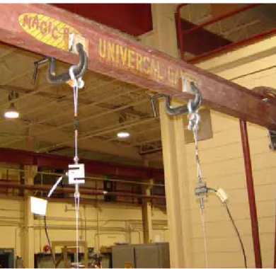
A gantry was erected over the trim tank in the AUV lab. This gantry was extended so that its beam was 2.5 metres above the floor. Two pinch clamps were constructed and clamped to the beam for the dry bifilar swinging. These clamps provide an exact point for the origin of the swing and allow the wires to be adjusted so that the vehicle was level during swinging. We attempted to use these clamps for swinging the flooded model, but they failed under the added weight and a system of clamps and slings was used instead.

(11)

Figure 5 - Dry Swing Apparatus

Figure 6 - Close up View of Pinch Clamp

For the in-water measurements (buoyant force and CG in water) a different apparatus was used. This involved suspending the models from two load cells hanging from the gantry. This allowed us to locate the center of gravity, position the slings equally on either side and take measurements without taking the model out of the apparatus. The clamp and sling arrangement is shown below.

(12)

Figure 7 - Apparatus for Wet Model Measurements

The load cells shown are 100 lb (45 kg) rated load cells that were connected to a data acquisition system. This allowed us to see what the weights were in real-time and record them to file as well.

For the buoyant weight and CG of the model additional slings were added so the entire model was submerged when measurements were taken. Once this was completed, the model was raised from the water using the overhead crane and those slings removed to allow the model to be flooded and swung.

Measurements

All the measurements were conducted on each configuration, then that configuration was disassembled, another assembled and each of the tests repeated. The basic sequence of events was to first assemble and photograph the model. Next the length of the model was measured and the location of the dry CG found.

(13)

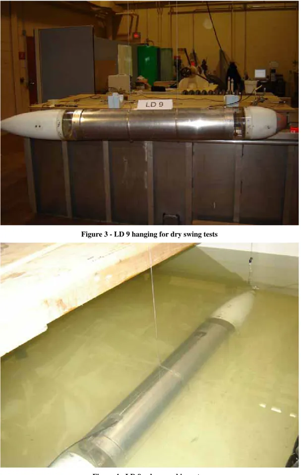
Next the model was placed in the filaments and hung from the grip clamp apparatus described above. The model was set into oscillation and the period of this oscillation measured. This completed the dry measurements.

The vehicle was then placed in different slings for the wet portion of the tests. It was then submerged in the water. The two loadcells were positioned such that each was in tension and reading a value. The underwater CG was found by moving the slings until the two load cells showed the same reading, thus each loadcell supported half the vehicle’s weight; the CG is then at the midpoint of the two slings. In some cases this required positioning the aft sling close to the end of the tail cone and the forward sling near the middle of the vehicle. The vehicle was then carefully lifted from the tank using the overhead crane. Car must be taken during this step, because the CG of the vehicle under water is different then the CG of the flooded vehicle in air. As the vehicle is lifted from the water, the flood water drains from it, changing its CG again.

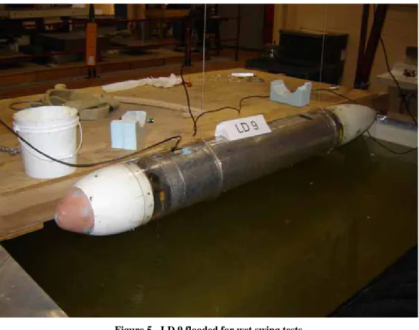
The sling length was then shortened and the vehicle hung, over the water from the load cells. With the slings located 60 cm apart the vehicle was flooded with water. Provided the seams of the vehicle are sealed with vinyl tape and the tail section plugged, leaking should not be a significant problem. Once the vehicle is flooded, note the readings on the two load cells and use them to locate the CG of the flooded model. Reposition the slings so that they are equally spaced on either side of the CG. While repositioning the sling water will likely spill from the vehicle and the floodwater will need to be topped up and the load cells read again to confirm that the slings are spaced properly. With the slings positioned and the vehicle completely filled with water, the vehicle was again oscillated and the period of oscillation measured.

There was some concern as to the sensitivity of the bifilar measurements to such parameters as, the weight of the filaments, environmental conditions (ventilation fans), and the stiffness of the apparatus. To confirm that the measurements were yielding valid data, a round aluminum bar (1.454 m long, 12.7 kg) was swung from the apparatus. It was oscillated and timed is the same manner as the models. The period was then used to calculate a radius of gyration of 0.4187m.

Since this was a uniform homogeneous body, calculating it’s theoretical radius of gyration was straightforward, as shown below,

2 12

1

mL I =

Equation 2 - Moment of Inertia of a rod about its axis

(14)

m I K =

Equation 3 - Radius of Gyration - Theoretical

12 2

L K =

Equation 4 - Radius of Gyration in terms of length

where:

I = Moment of Inertia (kg m2) m = Mass (kg)

K = Radius of Gyration (m) L = Length of the body (m)

This yields: m L K 0.4197 12 454 . 1 12 2 2 = = =

This shows that the apparatus and environmental conditions have a minimal effect on the overall calculation of the radius of gyration.

An attempt was also made to obtain a period of oscillation for the flooded model in water. The apparatus used for this was the same as the one used to swing the flooded model in air, but with longer slings. With the slings positioned an equal distance on either side of the CG the vehicle was set oscillating. The filaments in this case needed to be located very close to the CG to avoid being placed on the tapered portion of the tail section. This location, combined with the vehicle’s weight in water (40 N), produced a very weak restoring force. This caused the vehicle to return very slowly and to translate as well as oscillate about it’s CG. This made it impossible to measure the period with confidence.

(15)

Results

The results of the measurements are presented in full in Appendix A. A brief discussion of some of those results is presented here.

In general, due to the construction of the model, the center of gravity of the model in water was very near the aft cone piece. This is due to the addition of buoyant foam in the nose cone. The buoyant force of each flooded model ranged from 26 to 45 N.

Listed below are the length and mass, as well as the location of the CG for each configuration measured from the bow of the vehicle.

Table 1 - Length and mass measurements for each configuration

Configuration Length Mass (dry) Mass (flooded)

(m) (kg) (kg) LD 8 1.723 24.30 2.656 LD 9 1.927 25.60 3.171 LD10 2.125 27.30 3.792 LD11 2.334 28.20 4.04 LD12 2.535 29.80 4.549

Table 2 - CG locations for each configuration

Configuration CG (dry) CG (in water) CG (flooded in air)

(m) (m) (m) LD 8 0.734 1.287 0.847 LD 9 0.815 1.392 0.939 LD10 0.912 1.504 1.057 LD11 1.011 1.615 1.159 LD12 1.118 1.722 1.256 12

(16)

Based on the period of oscillation measurements the radius of gyration and moment of inertia were calculated for each model. This data is presented in Table 3 and Table 4.

Table 3 - Radius of Gyration for each configuration

Configuration DRY (in air) FLOODED (in air)

Radius of Gyration Radius of Gyration

(mm) (mm) LD 8 381 ± 1.41 423 ± 1.46 LD 9 419 ± 1.47 490 ± 1.87 LD10 447 ± 1.51 514 ± 1.68 LD11 489 ± 1.58 558 ± 1.73 LD12 529 ± 1.65 648 ± 2.08

Table 4 - Moment of Inertia for each configuration

Configuration DRY (in air) FLOODED (in air)

Moment of Inertia Moment of Inertia

(kg m2) (kg m2) LD 8 3.52 8.82 LD 9 4.49 13.25 LD10 5.44 16.73 LD11 6.73 21.84 LD12 8.34 32.36 13

(17)

Uncertainty Analysis

In an effort to determine the sensitivity of the final radius of gyration calculated from the measurements outlined above an uncertainty analyis was conducted based on the

following uncertainty levels in each measurement

Period of Oscillation: u (T) = ± 0.01 second Length of Filaments: u (L) = ± 0.003 meters Distance between Filaments: u (D) = ± 0.001 meters

L g TD K π 4 =

Base on Equation 1 (introduced previously and repeated here) the uncertainty in the radius of gyration value can be described as:

( )

u

( )

L L K D u D K T u T K K u2( ) 2 2 ⎟ 2 ⎠ ⎞ ⎜ ⎝ ⎛ ∂ ∂ + ⎟ ⎠ ⎞ ⎜ ⎝ ⎛ ∂ ∂ + ⎟ ⎠ ⎞ ⎜ ⎝ ⎛ ∂ ∂ =

Equation 5 - Radius of Gyration Uncertainty

where:

u = Uncertainty in a given measurement T = Period of Oscillation (s)

K = Radius of Gyration (m) L = Length of the body (m)

The partial derivatives of the radius of gyration with respect to each measurement are listed below: T K L g D T K = = ∂ ∂ π 4

Equation 6 - Partial Derivative of K with respect to T

D K L g T D K ₌ ₌ ∂ ∂ π 4

Equation 7 - Partial Derivative of K with respect to D

(18)

⎟ ⎠ ⎞ ⎜ ⎝ ⎛ = ⎟ ⎠ ⎞ ⎜ ⎝ ⎛ = ∂ ∂ − 2 1 2 1 * 4 2 3 L K L g TD L K π

Equation 8 - Partial Derivative of K with respect to L

Equations five to eight can be combined to give the following equation:

( )

⎥ ⎥ ⎦ ⎤ ⎢ ⎢ ⎣ ⎡ ⎟ ⎠ ⎞ ⎜ ⎝ ⎛ + ⎥ ⎥ ⎦ ⎤ ⎢ ⎢ ⎣ ⎡ ⎟ ⎠ ⎞ ⎜ ⎝ ⎛ + ⎥ ⎥ ⎦ ⎤ ⎢ ⎢ ⎣ ⎡ ⎟ ⎠ ⎞ ⎜ ⎝ ⎛ = ( ) 4 1 2 2 2 2 2 2 2 L u L K D u D K T u T K K u

Equation 9 - Discrete Uncertainty Equation

Based on the uncertainty levels listed above for each measurement, and Equation 9, the uncertainty of each radius of gyration calculation was found. These uncertainties ranged from 1.5 mm to 1.8 mm for the different configurations.

(19)

Conclusions

The primary conclusion of the measurements taken from this exercise is the values of the parameters outlined in the ‘Results’ section above. As outlined above, this procedure is an effective method of determining the radius of gyration of flooded and dry underwater vehicles. This method can be done for either yaw (as outlined here), pitch or roll using the same procedure, but changing the orientation of the vehicle.

Recommendations

Determining the various parameters listed here could be made easier in the future if the following guidelines are followed:

When material is used to fill the void space inside the model, wherever possible use equal amounts in the forward and aft portions of the vehicle. In the case of the Phoenix model the location of the CG underwater (very near the aft cone) made it difficult to take some measurements. This could have been rectified if the foam that was used in the nose cone had been offset with an equal volume of foam in the tail portion.

Where internal bulkheads (stainless steel rings in this case) are used and are not

separating watertight compartments, drill holes through the top of those bulkheads. This would allow air to move from one compartment to another when the vehicle is being submerged. This makes it easier to eliminate air bubbles when the vehicle is placed in the water for buoyancy measurements.

(20)

References

Card, Taran. Bifilar Swinging Experiment. Institute for Ocean Technology. LM-2000-01.

Hyperphysics, Department of Physics and Astronomy, Georgia State University.

http://hyperphysics.phy-astr.gsu.edu/hbase/mi.html

Hall, Tom. Institute for Ocean Technology. Personal conversation regarding bifilar swinging. Nov. 29, 2005.

Harnum, Enos. Institute for Ocean Technology. Personal conversation regarding assembly of acrylic pieces for Phoenix configurations. Nov. 21, 2005.

(21)

Appendix A: Spreadsheets of Results from Phoenix Model

Measurements

(22)

(23)

(24)

(25)

(26)

(27)

(28)

(29)

(30)

(31)

(32)

(33)

(34)

(35)

(36)

(37)

Appendix B: Photos of Each Configuration

(38)

(39)

(40)

(41)

(42)

(43)

Phoenix model measurement and bifilar swinging

Archives des publications du CNRC

PHOENIX MODEL MEASUREMENT AND BIFILAR SWINGING

Summary

Table of Contents

List of Figures

List of Equations

List of Tables

Background

Configurations

Apparatus

Measurements

Results

Uncertainty Analysis

( )

( )

( )

( )

( )

( )

Conclusions

Recommendations

References

Appendix A: Spreadsheets of Results from Phoenix Model

Measurements

Appendix B: Photos of Each Configuration