Reducing Particle Filtering Complexity for 3D Motion Capture using Dynamic Bayesian Networks

(1)

HAL Id: inria-00332714

https://hal.inria.fr/inria-00332714

Submitted on 21 Oct 2008

HAL is a multi-disciplinary open access

archive for the deposit and dissemination of

sci-entific research documents, whether they are

pub-lished or not. The documents may come from

teaching and research institutions in France or

abroad, or from public or private research centers.

L’archive ouverte pluridisciplinaire HAL, est

destinée au dépôt et à la diffusion de documents

scientifiques de niveau recherche, publiés ou non,

émanant des établissements d’enseignement et de

recherche français ou étrangers, des laboratoires

publics ou privés.

Reducing Particle Filtering Complexity for 3D Motion

Capture using Dynamic Bayesian Networks

Cédric Rose, Jamal Saboune, François Charpillet

To cite this version:

Cédric Rose, Jamal Saboune, François Charpillet. Reducing Particle Filtering Complexity for 3D

Mo-tion Capture using Dynamic Bayesian Networks. Twenty-Third Conference on Artificial Intelligence

- AAAI-08, Jul 2008, Chicago, United States. �inria-00332714�

(2)

Reducing Particle Filtering Complexity for 3D

Motion Capture

using Dynamic Bayesian Networks

C´edric Rose

Diat´elic SA

INRIA Nancy - Grand Est

LORIA, FRANCE

cedric.rose@diatelic.fr

Jamal Saboune

INRIA Nancy - Grand Est

LORIA, FRANCE

jamal.saboune@loria.fr

Franc¸ois Charpillet

INRIA Nancy - Grand Est

LORIA, FRANCE

francois.charpillet@loria.fr

Abstract

Particle filtering algorithms can be used for the monitoring of dy-namic systems with continuous state variables and without any con-straints on the form of the probability distributions. The dimension-ality of the problem remains a limitation of these approaches due to the growing number of particles required for the exploration of the state space. Computer vision problems such as 3D motion tracking are an example of complex monitoring problems which have a high dimensional state space and observation functions with high compu-tational cost. In this article we focus on reducing the required number of particles in the case of monitoring tasks where the state vector and the observation function can be factored. We introduce a particle fil-tering algorithm based on the dynamic Bayesian network formalism which takes advantage of a factored representation of the state space for efficiently weighting and selecting the particles. We illustrate the approach on a simulated and a realworld 3D motion tracking tasks.

1 Introduction

Complexity and uncertainty are two common problems that arise when dealing with realworld monitoring applications. Markerless 3D motion tracking is an example of a high dimensional problem with partial observability. Partially observable Markov pro-cesses are a formal framework that allow probabilistic reasoning on dynamic systems.

(3)

Dynamic Bayesian networks are a graphical formalism that can be used to model dy-namic processes such as Kalman filter, hidden Markov Model and more generally any kind of Markov process over a set of variables. Exact or approximate deterministic inference algorithms are always based on assumptions over the form of the probability laws that govern the system. It is not the case for particle filtering that has the advan-tage of working with any kind of probability distributions. Particle filtering is known to perform exact inference asymptotically (for an infinite number of particles). In prac-tice, particle filtering is used to perform approximate inference with a limitation due to the dimensionality of the problem. In this article we focus on reducing the number of particles for problems that can be factored. We introduce a factored particle filtering inference algorithm for dynamic Bayesian network and its application on a simulated and a realworld 3D motion tracking problem.

2 Markov processes and particle filtering

In partially observable Markov processes, we assume that the probability distribution over the state space which is called the belief state is conditionally independent from the past sequence given the previous state.

P (Xt|X1:t−1) = P (Xt|Xt−1)

In the same way, the observation is conditionally independent of the past given the current state. The belief state can be computed recursively using the Bayes rule.

αt(xt) = P (Xt= xt|y1:t)

αt(xt) = P (yt|xt) P

xt₋₁P (xt|xt−1)αt−1(xt−1)

P (yt|y1:t−1)

The idea behind particle filtering is to represent the probability distribution over the state space by a weighted set of particles {xi_t}i=1..N _{sampled from a proposal}

distribution. αt(xt) ≈ N X i=1 wi_{tδ(xt, x}i_t)

whereδ is the Dirac delta function.

The particles are resampled and weighted in order to maintain the estimation of the belief state over time given the previous observations. The required number of particles grows as an exponential function of the dimensionality of the state space [4].

Condensation algorithm introduced by Isard et al. [3] is described in 3 steps. • The resampling step where a selection occurs among the particles associated to

αt−1.

• The diffusion step which consists in estimating

P (xt|y1:t−1) = X xt₋₁

(4)

by moving the particles according to the dynamics of the system (described by

P (xt|xt−1) used as a proposal distribution).

• The measure step in which the weight of the particles are updated using the observationP (yt|xi_{t) and normalized. The normalization factor corresponds to}

1 P(yt|y_1:t−1).

3 Working with a small number of particles

Particle filtering in a continuous state space is an example were the exploration ex-ploitation dilemma occurs. The resampling step in the condensation algorithm ensures that more exploration effort will be spent on more likely state space areas at the cost of less precision in less likely areas. The difficulty here, particularly when working with multi-modal distribution, is to keep a sufficient exploration potential in order to find the global maximum. Reducing the number of particle is therefore a delicate matter, although it is often necessary for applications with high computational cost such as vision problems. In [1] the authors have used simulated annealing in order to simplify and incrementally refine the form of the state probability distribution and be able to keep track of the global maximum. In [6], the authors have used a modified particle filtering algorithm based on a deterministic exploration of parts of the state space. It shows the efficiency of deterministic distribution sampling when working with a small number of particles. In this article we propose to take advantage of the factorization of the probability distribution in order to reduce the number of particles. This factored approach can be combined with the previously mentioned methods.

4 DBN

Bayesian networks (BN) are a graphical formalism for reasoning about variables inde-pendence. A BN gives a graphical representation of the joint probability distribution of a set of variables. Each variable is described by a local probability law so that the joint probability distribution can be written as the product of the local laws. When work-ing with a time-evolvwork-ing set of variablesXt, we call the BN a Dynamic Bayesian Network (DBN). A DBN [5] is a temporal probabilistic model which is based on a factored representation of the probability distributionsP (Xt|Xt−1) and P (Yt|Xt)

where Xt andYt are decomposable into several variables: Xt = (X1

t, .., XtN) and Yt = (Y1

t, .., Y M

t ). The factored representation of P (Xt, Yt|Xt−1) is given by a

di-rected acyclic graph in which each node is associated to a variableXi torY j t. P (Xt, Yt|Xt−1) =Y i P (X_{t|P a(X}i _{t)) ×}i Y j P (Ytj|P a(Y j t)) whereP a(Xi t) ∈ (Xt−1, Xt),P a(Y j

t) ∈ (Xt) are the parents of Xti,Y j

t in the directed

acyclic graph.

Several exact and approximate deterministic inference algorithms exist for Bayesian networks according to the nature of the conditional probability distributions (discrete,

(5)

continuous linear gaussian, hybrid). In this article we propose a particle filtering al-gorithm for making inference in DBNs in the case of continuous variables with no constraints on the form of the probability distribution. With this algorithm we intend to reduce the number of particles required for finding the most likely values of the hidden variables given an observation sequence.

5 Factored Particle Filtering

A critical issue in high dimensional particle filtering is that a majority of the particles get ’killed off’ during resampling step, meaning that a lot of the exploration effort is wasted. The main idea behind this work is to use the factorization of the process for hierarchically resampling the components of the state vector. Our proposal is inspired by the likelihood weighting procedure [2][7] in which the elements of the state vector are sampled in a topological order. We denote asxi

ttheithparticle at timet which is

an instantiation of the whole set of variables of the DBN. Thenth_{variable of the DBN}

being denoted asXn

t, the particlexitis an instantiation of(Xt1, ..., XtN). By searching

the graph in a topological order, we propose to resample the particles every time an observed node is encountered. Thus, the particles can be eliminated without being fully instantiated and the early resampling improves the efficiency of the exploration effort.

• If the node corresponds to a state variableXn

t, each particlexitis completed with

a sample from the proposal distributionP (Xn

t|P a(Xtn) = ui) where uiis the

value ofP a(Xn

t) in the particle xitor its predecessor at timet − 1.

• If the node corresponds to an observation function. The weightwi

tof the particles xi

tis updated by the rule : wi t= w i t∗ P (Y k_{= y}k t|P a(Y k t ) = ui)

whereuiis the value ofP a(Yk

t ) in particle xit. If necessary the particlesxitare

resampled according to their weightwi t.

Figure 1: Hierarchical resampling: Grey nodes correspond to particles with higher weight after introduction of observationYi.

Figure 1 is an illustration of the resampling process. The algorithm is detailed in figure 2.

(6)

P a(xi_{t) : parent particle at time t − 1 of particle i.}

Zt=(Xt,Yt) denotes the set of observed and hidden variables.

N is the total number of particles.

For each node n in topological order case n hidden

for each particle i

ui= value of (Pa(Zn

t)) in (xi,P a(xit))

Completexi

twith a sample fromP (Ztn|P a(Ztn) = ui)

case n observed (Zn₌_yk t)

for each particle i

ui= value of (Pa(Zn

t)) in (xi,xt−1) wi

t= wit∗ P (Zn= ytk|P a(Ztn) = ui)

resample the particles according to their weightw∗ t = 1/N

Figure 2: Factored particle filtering algorithm.

6 3D Motion tracking

In this section we show how we can use factored particle filtering in an application of 3D motion tracking. 3D motion tracking can be viewed as a Markov monitoring task in which we search the most likely state sequence of the 3D model knowing an observation sequence given by video feeds.

6.1 Factored representation of a kinematic chain

A kinematic chain is defined by a set of joints between segmentsSi

i=1..Nallowing

rel-ative motion of the neighboring segments. The state of the chain can be described by the relative positions of the neighboring segments which we denote as{R1, ..., RN_}.

The dimensionality of the each relative positionRi_{depends on the degrees of freedom}

of the corresponding joint. In an open loop chain, every segment of the chain is con-nected to any other segment by one and only one distinct path and the chain takes the form of a tree. We can define a hierarchy between the joints by taking one of the seg-ments as the root of the structure. We denote the absolute 3D position of the segseg-ments in topological order as{X0_{, ..., X}N_{} and P a(X}i_{) refers to the position of the parent}

of theith_segment.

The position of theit_{h segment X}i_{= fi(P a(X}i_{), R}i_{) can be calculated knowing}

the absolute position of its parent and the configurationRi_{of the joint linking}_Xi_and P a(Xi_{). Thus, the structure of the kinematic chain induce a factored representation}

of the joint probability distributionP (X0_{, ..., X}N_{) = Π}N

i=0(P (Xi|P a(Xi))). The

dimensionality of each factorP (Xi_{|P a(X}i_{)) is the same as the dimensionality of the}

corresponding jointRi_{. This factored representation is a Bayesian network in which}

(7)

dynamics.

6.2 Factored observation function

Our observation function is simply based on the video feeds. The basic idea is to compare the video inputs which are the projections of the ’real’ observed object to the projections of our 3D model. This doesn’t provide a direct observation of the segments. Nevertheless, we will show that the evaluation function can be factored. We can indeed evaluate the matching of the segments, not independently, but one after the other. The first segmentS1is compared to the reference image provided by the camera. The common pixels between the projection ofS1 _{and the silhouette are marked as}

masked and the resulting image is used as a reference for the next segment. This chain process for evaluating the state vector allows us to write the observation function as

P (Y |X) = ΠN

i=1P (Yi|Xi, pre(Yi)) where pre(Yi) is the observation function that

precedeYi_{in our evaluation process.}

7 Simulated hand gesture tracking

This section presents an experiment that we used for the validation of the algorithm. We developed a 3D articulated hand-like model which was used for the generation of motion sequences recorded by several virtual cameras. Performing this ’simulated motion tracking’ presents the advantage of knowing the corresponding exact state se-quence and provides the possibility to compare the 3D filtered positions to the exact 3D positions. It also allows us to avoid some image processing tasks (such as shadow filtering or silhouette extraction) as the sole evaluation of the algorithm itself is done in this part.

Figure 3: 3D hand-like model

The used model contains 15 degrees of freedom represented by 15 variables. The only presumed dynamic constraints are angular speed limits for each joint. Therefore, the conditional density distributions are uniform laws on intervals centered on the rel-ative position of the joints a timet − 1.

Combining factored particle filtering with deterministic interval sampling [6], we used a simple particle resampling method which consists in keeping at each rank the 5 most fitting particles and copy them 5 times for diffusion without uniformizing their weight so that the sumPN_i=1wi_{tδ(xt, x}i_{t) remains proportional to αt(xt). For particle}

(8)

diffusion we sampled the uniform laws deterministically taking 5 samples equally dis-tributed on the interval. As a result, the number of particles oscillates between 5 and 25 and the total number of particles evaluated for each time step is15 × 25 = 375. This

way of diffusing the particles, which differs from the method used in the condensation algorithm, ensures a minimum exploration potential which is needed in compensation to the reduction of the number of particles.

The animated scene was recorded from different view points by 3 virtual cameras. The results of the tracking performed using375 particle estimations per frame were

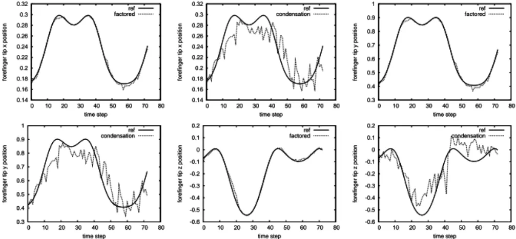
visually satisfying. We measured the error relatively to the amplitude of the movements by dividing the euclidean distance between the tracked 3D positions and the true 3D positions of each joints by the amplitude of their movement. The error calculated for each joint was then averaged over time. Using factored particle filtering, we obtained a 4% average error calculated over all the 3D points. As a comparison, the condensation algorithm using the same number of particles (375) resulted in a 13% average relative error. An example of a comparison between condensation and factored particle filtering is given on figure 4. The true 3D position of the tracked point is given as a reference. Even using a relatively small number of particles, condensation manages to keep track of the finger movement but it is clearly outperformed by the factored approach. On the forefinger tip, the reconstruction average error is 2% for the factored approach while it is 19% in the case of condensation.

0.14 0.16 0.18 0.2 0.22 0.24 0.26 0.28 0.3 0.32 0 10 20 30 40 50 60 70 80

forefinger tip x position

time step ref factored 0.14 0.16 0.18 0.2 0.22 0.24 0.26 0.28 0.3 0.32 0 10 20 30 40 50 60 70 80

time step ref condensation 0.14 0.16 0.18 0.2 0.22 0.24 0.26 0.28 0.3 0.32 0 10 20 30 40 50 60 70 80

time step ref condensation 0.3 0.4 0.5 0.6 0.7 0.8 0.9 1 0 10 20 30 40 50 60 70 80

forefinger tip y position

time step ref factored 0.3 0.4 0.5 0.6 0.7 0.8 0.9 1 0 10 20 30 40 50 60 70 80

time step ref condensation 0.3 0.4 0.5 0.6 0.7 0.8 0.9 1 0 10 20 30 40 50 60 70 80

time step ref condensation -0.6 -0.5 -0.4 -0.3 -0.2 -0.1 0 0.1 0.2 0 10 20 30 40 50 60 70 80

forefinger tip z position

time step ref factored -0.6 -0.5 -0.4 -0.3 -0.2 -0.1 0 0.1 0.2 0 10 20 30 40 50 60 70 80

time step ref condensation -0.6 -0.5 -0.4 -0.3 -0.2 -0.1 0 0.1 0.2 0 10 20 30 40 50 60 70 80

time step ref condensation

Figure 4: 3D reconstruction: comparison between forefinger tip reference and tracked positions using factored particle filtering (on left) and using condensation (on right).

8 Human motion tracking

3D human motion capture systems are based on an estimation of the 3D movements of some points of the body. Marker-based systems have been widely used for years with applications found in biometrics or animation. These approaches implicate the use of expensive specialized equipments and require a footage taken in a specially arranged

(9)

environment. Using video feeds from conventional cameras and without the use of special hardware, implicates the development of a marker less body motion capture system. Research in this domain is generally based on the articulated-models approach. This section shows the feasibility of applying factored particle filtering to 3D human motion capture.

8.1 The articulated body model and the likelihood function

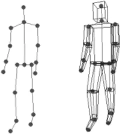
The 3D articulated human body model we use simulates the human movement through the configuration of 31 degrees of freedom. These degrees of freedom represent rota-tions of 19 joints of the body (neck, elbows, knees etc..). The body parts form an open loop kinematic chain composed of four branches starting from the torso.

Figure 5: 3D articulated human body model composed of 19 joints each represented by a 3D point.

In addition to defining a model, we define a function to evaluate its configuration (31 parameters values) likelihood to the real image. A silhouette image of the tracked body is constructed by subtracting the background from the current image and then applying a threshold filter. This image will then be compared to the synthetic image representing the model configuration (2D projection of the 3D body model) to which we want to assign a weight. This evaluation can be made in a factored manner as explained before by projecting the body parts sequentially and masking previously observed segments on the real image.

(10)

8.2 DBN for human motion capture

The corresponding dynamic Bayesian network is adapted from the kinematic chain representation of the model by choosing the torso position as the root variable for directing the edges. Edges have also been added between the observed nodesYk to show the dependences (hierarchical order) between the observation functions. In order to take advantage of the factored representation of the state vector, the hierarchy of the observations has to follow the one of the hidden variables. For separate branches (right leg, left leg,...) an order is defined arbitrarily. The dynamics of the different joints are specified by temporal links between variables at timet − 1 and variables at time t. A

partial representation of the DBN is shown on figure 7.

No dynamic nor trained walking models were used, which makes this approach simple and generic. The only dynamic constraints used are those of the human body joints (amplitude and speed limits). For each joint, the proposal distribution is a uni-form probability density function covering an interval centered on the previous position of the joint. The width of the interval depends on the physiological joint speed limit.

Figure 7: A (partial) DBN for gait analysis, based on the kinematic chain of a 3D articulated body model. Grayed nodes (Yi) correspond to observation functions. The parts of the kinematic chain corresponding the arms are missing on this representation for simplification reasons.

8.3 Recovering from ambiguous situations

There are several sources of ambiguities when working on real-world motion tracking. The limited number of different viewpoints results in sequences where certain part of the body are occluded. The enlightenment of the scene is usually not uniform. The background color may produce imperfect silhouette extraction. The capacity of the

(11)

algorithm to recover from these ambiguities is related to its capacity to represent the uncertainty about the state variables. This capacity closely depends on the number of surviving particles at each resampling step.

In [6], the authors used a simple method for ensuring occlusion recovery while re-ducing the number of particles. The idea is to ensure a minimum exploration effort by injecting static particles in the state space. This method can be adapted to the factored approach by injecting complete configurations or variable configurations. Particle in-jection can compensate the risk of using a small number of particles.

On figure 8, we have compared the evolution of the algorithm from a single mis-placed particle. On the left, the algorithm evolves using the uniform proposal distribu-tion based on the joint speed limits. On the right, a few static particles (2%) are added. In the two cases, the five best particles were kept after each resampling step.

Figure 8: Recovering from a misplaced particle.

8.4 Discussion

In our experiments we used two video cameras with a resolution of780 × 580 working

at 25Hz. The factored approach allows visually satisfying motion tracking with a re-duced number of particles. Less than 800 particles were necessary for the tracking of the 17 degrees of freedom on which gait movement is based. 2000 particles are neces-sary for the full 31 degrees of freedom motion tracking. This constitutes a significant improvement in comparison to the original Interval Particle Filtering [6] using 6000 particles.

(12)

The observation function is rather simple and the whole motion tracking process rely on the quality of silhouette extraction (shadow removal, thresholding, ...). The number of video feeds used is also a critical element for eliminating occlusion prob-lems. In our experiments, only the five best particles where kept after each resampling step. We used static particles injection in order to ensure that the tracking did not di-verge in the case of ambiguous observations for which keeping only five particles at resampling step may not be sufficient.

9 Conclusion

We have presented a new approach for 3D motion estimation using the formalism of dynamic Bayesian networks and a modified particle filtering algorithm for taking ad-vantage of the factorization of the state space. The observation at time stept is used for

the generation of the particles at timet which allows to search the state space more

effi-ciently by reducing the exploration of unlikely areas. The particle economy rely on the capacity for the observation function to be factored in accordance with the state vector. We showed that the structure of a kinematic chain induced a factored representation of the probability distribution over its configurations which is based on dynamics of its joints. We saw that the likelihood function in an articulated-model approach could be factored. Using these results we were able to address a 15 degree of freedom problem using 15 layers of 25 particles each which represents only375 particles estimations.

On real human motion tracking, the number of particles was significantly reduced due to the use of factored particle filtering.

Acknowledgements

The authors would like to thank Abdallah Deeb, engineer at INRIA Nancy Grand Est, for his participation to this work. This project has been partially funded by the ANR (French National Research Agency), Tescan program, PreDICA project.

References

[1] J. Deutscher, A. Blake, and I. Reid. Articulated body motion capture by annealed particle filtering. In Computer Vision and Pattern Recognition, volume 2, pages 126–133, Hilton Head Island, SC, USA, 2000.

[2] Robert M. Fung and Kuo-Chu Chang. Weighing and integrating evidence for stochastic simulation in bayesian networks. In UAI ’89: Proceedings of the Fifth

Annual Conference on Uncertainty in Artificial Intelligence, pages 209–220,

Am-sterdam, The Netherlands, The Netherlands, 1990. North-Holland Publishing Co. [3] Michael Isard and Andrew Blake. Condensation – conditional density propagation

(13)

[4] John MacCormick and Michael Isard. Partitioned sampling, articulated objects, and interface-quality hand tracking. In ECCV ’00: Proceedings of the 6th

Eu-ropean Conference on Computer Vision-Part II, pages 3–19, London, UK, 2000.

Springer-Verlag.

[5] Kevin Patrick Murphy. Dynamic Bayesian Networks : Representation, Inference

and Learning. PhD thesis, University of California Berkeley, 2002.

[6] J. Saboune and F. Charpillet. Using interval particle filtering for marker less 3d human motion capture. In 17th IEEE International Conference on Tools with

Arti-ficial Intelligence, pages 621–627, Hong Kong, 2005.

[7] Ross D. Shachter and Mark A. Peot. Simulation approaches to general probabilis-tic inference on belief networks. In UAI ’89: Proceedings of the Fifth Annual

Conference on Uncertainty in Artificial Intelligence, pages 221–234, Amsterdam,