A Decomposition Algorithm for Local Access Telecommunications Network Expansion
Planning Anantaram Balakrishnan, Thomas L. Magnanti and Richard T. Wong WP# 3496-92-MSA September, 1992
A Decomposition Algorithm for
Local Access Telecommunications Network
Expansion Planning
Anantaram Balakrishnan*§
Thomas L. Magnanti §
Sloan School of ManagementM. I. T. Cambridge, MA
Richard T. Wong
AT&T Bell LaboratoriesHolmdel, NJ
Revised: September 1992
t This research was initiated through a grant from GTE Laboratories Incorporated, Waltham, Massachusetts
Abstract
Growing demand, increasing diversity of services, and advances in transmission and switching technologies are prompting telecommunication companies to rapidly expand and modernize their networks. This paper develops and tests a
decomposition methodology to generate cost-effective expansion plans, with performance guarantees, for one major component of the network hierarchy-the local access network connecting customers to the local switching center. The model captures economies of scale in facility costs, and addresses the central tradeoff
between installing concentrators and expanding cables to accommodate demand growth. By exploiting the special tree and routing structure of the expansion
planning problem, our solution method integrates two major algorithmic strategies from mathematical programming-the use of valid inequalities, obtained by
studying a problem's polyhedral structure, and dynamic programming, which can be used to solve an uncapacitated version of the local access network expansion
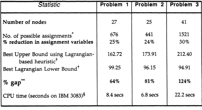
planning problem. The computational results for three actual test networks
demonstrate that this enhanced dynamic programming algorithm, when embedded in a Lagrangian relaxation scheme (with problem preprocessing and local
improvement), is very effective in generating good upper and lower bounds: implemented on a personal computer, the method was able to generate solutions that are within 1.2 to 7.0% of optimality. In addition to developing a successful solution methodology for a practical problem, this paper illustrates the possibility of effectively combining decomposition methods and polyhedral approaches.
Keywords: Integer programming decomposition, concentrator location, telecommunications planning, polyhedral methods
1. Introduction
Advances in switching and transmission technologies combined with growing demand, increasing diversity of services, and deregulation of the
telecommunications industry have prompted telephone companies to rapidly upgrade and expand their networks. Modernization of the local access networks, which connect switching centers to customers, is a particularly important priority since these networks account for over 50% of the total investment in
communication facilities (according to Standard and Poor's Industry Surveys [1992], the total value of plant in 1990 exceeded 250 billion dollars in the U. S. alone); yet they are not as technologically advanced as the higher levels-the long-distance and inter-office networks-in the telecommunications network hierarchy. For instance, over 80% of the local access networks still use analog transmission over copper cables. However, recent technology and cost trends in the industry have improved the economic and technical viability of introducing electronic switching and fiber optic transmission to increase capacity in local access networks.
The new technologies such as electronic remote units (or multiplexers) introduce discrete choice decisions and spatial couplings between different parts of the
network, thus vastly increasing the number of possible ways to meet growing demand. Traditional manual planning methods that consider only the option of adding more cables to expand capacity are no longer adequate. Since
telecommunication investments are so expensive (total annual investments by U. S. local exchange companies is approximately $20 billion, Telephony [1991]), a cost effective network expansion plan can offer considerable economic value. For
instance, Jack, Kai, and Shulman [1992] report savings of over $30 million per year at GTE using an interactive decision support system to assist network planners.
This paper develops and tests an optimization-based methodology to identify a minimum cost network expansion plan to meet increasing demand. We formulate an integer programming model, validated by consulting network planners in
industry, that captures the essential tradeoffs between concentrator location and cable expansion, and accommodates economies of scale in investment and operating costs. Although the model approximates the expansion costs as piecewise-linear concave functions, and does not consider investment timing decisions, it is an important building block for detailed, multi-period planning systems (see, for example, Shulman and Vachani [19901). To solve the local access network expansion model, we develop a decomposition method combining Lagrangian relaxation with a dynamic programming algorithm that exploits the problem's special tree structure and routing restrictions. Since the basic problem formulation does not provide satisfactory lower bounds, we identify several classes of valid inequalities that strengthen the model's linear programming relaxation. Unlike other cutting plane methods that use general purpose linear programming codes to solve the enhanced
formulations (e.g., Hoffman and Padberg [1985]), we modify the dynamic programming algorithm to directly incorporate the valid inequalities. Our
computational tests using representative data (obtained from industry) demonstrate that the method generates good upper and lower bounds. Thus, this paper not only develops an effective solution method for the important practical problem of local access network design, but also adds to the growing literature demonstrating the usefulness of polyhedral methods for solving difficult, large-scale optimization problems.
The rest of this paper is organized as follows: Section 2 presents a formal definition of the local access network planning problem, reviews our modeling assumptions, and describes a basic mixed-integer programming formulation. Section 3 describes an efficient dynamic programming algorithm to solve the uncapacitated version of the local access network planning problem, develops a Lagrangian relaxation scheme that uses the dynamic program to solve an
uncapacitated subproblem, and outlines a Lagrangian-based heuristic procedure. In Section 4 we describe two algorithmic enhancements-a problem preprocessing procedure to eliminate variables, and a coefficient reduction method to strengthen the problem formulation. Section 5 presents three classes of valid inequalities, and shows how to modify the dynamic program to incorporate them. Section 6 describes our implementation, and presents computational results for three networks
provided to us by a major telephone company. We illustrate how the valid inequalities dramatically improve the lower bounds (by about 80%) relative to the basic model, and we study the robustness of the method to changes in demand and cost parameters. Our results show that the combination of Lagrangian relaxation, dynamic programming, and polyhedral methods permits us, using a personal computer, to efficiently find solutions that are within 1.2 to 7.0% of optimality. Section 7 identifies directions for further work.
2. The Basic Local Access Network Expansion Model
2.1 Problem description
The local access network (also called the feeder loop, central office network, outside plant, or customer access network) connects customer nodes (control or distribution points, in telecommunication parlance) to the switching center (also called the central office). Each customer node is a collection point for individual customers (possibly hundreds) connected via a subsidiary distribution network. Balakrishnan et al. [19911 and Jack et al. [1992] describe the technologies and characteristics of local access networks in greater detail. Most current local access networks have a tree structure, rooted at the switching center (Shulman and
Vachani [19901). Edges of the tree correspond to physical sections of underground or overhead cables.
All communications to and from each customer node flow through the assigned switching center. Each node has a demand, measured by the required number of circuits from that node to the switching center. In conventional copper networks, each circuit requires a dedicated twisted copper pair which we will call a cable. A node's demand depends on the number and type (e.g., residential or commercial) of individual customers connected to it. The local access network can satisfy this demand in two ways: either provide a dedicated cable (from the customer node to the switching center) for each required circuit, or route the circuits through a traffic compression device called a concentrator. Concentrators are electronic devices that combine incoming signals (e.g., analog signals) on several lines into a single
composite signal (e.g., high frequency digital or optical signal) that requires only one outgoing line. In practice, a variety of devices such as electronic multiplexers, remote switches, and fiber optic terminals can perform traffic compression (see Balakrishnan et al. [1991]). We collectively refer to all these different technologies as concentrators. Our planning model distinguishes between different technologies through their installation and operating cost functions.
As customer demand increases (for example, due to new construction, customer movement, or new services), the existing cables and concentrators can no longer accommodate the required number of circuits from each node. In the expansion planning problem, we wish to locate new concentrators, selectively expand cable capacities, and reroute traffic from customer nodes via concentrators in order to satisfy the projected demand using the minimum possible total network expansion cost. By routing traffic through concentrators, we reduce the downstream (or central office side) cable requirements. This tradeoff between installing concentrators and expanding cable capacities is central to the local access network expansion problem. We next introduce some notation and formally describe the expansion planning model and its assumptions.
Notation and problem parameters
Let T denote the given (undirected) rooted tree over which the local access network expansion problem is defined. The nodes of this network represent
customer nodes and/or potential concentrator locations, and its edges correspond to cable sections. We index the set of nodes N from 0 to n, with the root node 0
representing the switching center. Let didenote the projected demand at each
customer node i. The capacity Bij of edge (i,j) is the number of existing cables in the section connecting nodes i and j. For simplicity, all our subsequent discussions assume that the existing network does not contain any concentrators; however, our method extends easily to problems with existing concentrators.
Let Pij denote the (unique) path in the tree connecting nodes i and j. To provide one circuit from node i to the switching center, we must reserve one cable on each edge of the path Pi0. Since the existing network does not have adequate capacity to
meet the projected demand, one or more edges of the current network must have projected exhaust, i.e., the number of available cables on that edge is less than the total demand for all nodes communicating through that edge to the switching center.
Cost structure
Our model minimizes the total cost of installing concentrators and adding cables to meet the projected demand. The model and solution methodology can also incorporate additional node-to-concentrator connection costs (e.g., to disconnect the current circuit and reroute it through a concentrator at a different location) which we ignore for simplicity. Cable expansion costs vary by edge (depending on the length and location of the cable section), and has both a fixed and variable component. On each edge (i,j), we incur a fixed cable cost Gij (e.g., to install additional ducts or poles) and a variable cable cost eij that might represent, for instance, investment in cables or maintenance expenses. Concentrator costs also have location-dependent fixed and variable components. The fixed concentrator cost Fj models land acquisition and infrastructure investments at node j, while the variable concentrator cost cj reflects the purchase price and operating expenses of concentrator modules. As we note later, the concentrator cost also includes the cost of the required high-speed concentrator-to-switching center connection.
Our solution procedure also applies when concentrator and cable expansion costs have the more general piecewise-linear, concave structure shown in Figure 1; each segment in this function might correspond, for instance, to a different concentrator technology or transmission medium. The true cost of concentrators (or cable
expansion) is a step function of the required capacity since concentrator modules are available only in discrete units; however, our analysis of actual cost estimates and information provided by our industrial collaborator suggest that a piecewise-linear, concave function can adequately approximate this cost especially for long-term planning purposes (due to rapid technological changes, predicting the costs exactly for, say, a 5-year time horizon is often very difficult). Although we have
implemented and tested the solution method for problems with concave
concentrator costs, for expositional ease in describing the model formulation and solution algorithm, we will assume the simpler fixed plus variable cost structure for both cable expansion and concentrator location. (We do, however, indicate how the approach will handle concave costs.)
2.2 Modeling assumptions
To reduce the complexity of managing and maintaining the local access network, planners often impose several restrictions on the permissible expansion options and routing patterns. Discussions with planners in industry suggest that the following four modeling assumptions reflect or adequately approximate current practice.
Shulman and Vachani [1990] and Jack et al. [1992] use similar assumptions in their successful decision support system for local access network planning.
Assumption Al: Single-level concentration
Traffic originating at any node of the network is concentrated at most once before reaching the switching center.
Assumption A2: Non-bifurcated routing
A single concentrator (or the switching center) processes the entire demand of each customer node.
Assumption A3: Contiguity restriction
Every concentrator serves a contiguous region surrounding it, i.e., if a concentrator at node j serves node i, then this concentrator also serves all other nodes (including node j) on the connecting path Pij.
Assumption A4: Transmission cost for concentrated traffic
Concentrated traffic (flowing from each concentrator to the switching center) either consumes a negligible amount of existing cable capacity, or uses a dedicated umbilical connection (also called a remote-to-host connection) whose cost depends only on the location and throughput of the concentrator. In the latter case, we can incorporate the cost of the umbilical connection in the concentrator cost.
Assumption Al reflects current state-of-the-art in local access network design. Introducing multiple levels of concentration within the local access network is often uneconomical given the current costs of cables and concentrators. Assumptions A2 and A3 reflect operational convenience. For example, maintaining and repairing networks with multiple routes from each customer node or non-contiguous
concentrator service regions can be burdensome. Assumption A4 greatly simplifies the model and improves solution effectiveness, while introducing only minor distortions in total cost or actual capacity usage. For instance, one digital copper pair, also called a T1 span, can accommodate up to 96 voice channels (see, for example, Jack et al. [1992]); thus a customer node that previously required, say, 1000 copper
pairs for analog transmission, requires only 11 T1 spans to transmit compressed signals from that node. If the "concentrator" includes a fiber optic terminal, the fiber cable connecting the terminal to the switching center might replace an existing copper cable.
Since the local access network has a tree structure, assumptions Al and A2 together imply that assigning a concentrator (or switching center) to each node i completely specifies the routing decisions in the network. We say that node i homes on node j if a concentrator located at node j processes node i's traffic. In this case, the traffic from node i is routed on di cables along the unique path Pij to node j, where it
is concentrated and transmitted via the remote-to-host connection from node j to the switching center. Any node whose traffic is not concentrated is said to home on the switching center; equivalently, we assume that the switching center always has a concentrator. We permit backfeed or flow away from the switching center, i.e., a concentrator at node j can also serve downstream nodes that are closer than node j to the switching center. The contiguity assumption (A3) reduces the concentrator selection and assignment problem to one of decomposing (and covering) the tree into subtrees, and selecting one concentrator location within each subtree to serve its traffic requirements. We use this observation to efficiently solve an uncapacitated subproblem using dynamic programming.
To illustrate these concepts, consider the local access network shown in Figure 2. The dashed edges in this network are sections with projected exhaust. For instance, the current capacity of 1675 units on edge (26, 34) is less than the total demand (2203 units) of nodes 34 and 41. Hence, we must either expand this edge by 528 units in order to home nodes 34 and 41 on a downstream concentrator (or the switching center), or install a concentrator at either of these nodes. For instance, a concentrator at node 34 can serve both nodes 34 and 41. Since we permit backfeed, we can also home the downstream nodes, say nodes 26, 18, and 12, on this concentrator. Notice that, if we use this homing strategy, we need not expand edges (26, 34), (18, 26), and (12, 18) since their existing capacities can accommodate the required backflow. Also, if node 7 homes on the concentrator at node 34, the contiguity property specifies that node 13 (and node 19) cannot home on the switching center; this node must either home on node 34 or on a concentrator located at nodes 13 or 19.
2.3 Basic Integer Programming Formulation
In the local network expansion planning problem we consider, we are given the projected demand at each customer node, the existing cable capacity in each section, and the costs for adding cables and installing concentrators at each location. We need to decide:
* where to locate concentrators, and with what capacity; * which edges (cable sections) to expand, and by how much;
* how to route the traffic from each node to the switching center; and, * in a more general model, which concentrator technology to use at each
node.
Our formulation uses the following decision variables:
Assignment xij = 1 if node i homes on node j,
variable 0 otherwise;
Concentrator yj = 1 if we install a concentrator at node j,
location variable 0 otherwise;
Cable Zi (Zji) = 1 if we expand cable capacity from node i to
installation variable node j (node j to node i), 0 otherwise; and,
Cable ij (sj) = number of cables added from node i to node j
expansion variable (j to i).
We use directed variables to model cable installation and expansion, i.e., although edges are undirected, we distinguish between expansion in the i-to-j direction and the j-to-i direction on each edge (i,j). Using directed cable addition variables increases the formulation size but strengthens the model's linear programming relaxation, thus improving our algorithm's performance. To emphasize the direction of flow, we will consider two directed arcs, denoted as <i,j> and <j,i>, corresponding to each original undirected edge (i,j); both arcs have the same fixed and variable cable expansion costs as the original edge. We also redefine Pij as the directed path from node i to node j in the tree. We assume, for convenience, that each customer node can home on any other node in the network. In practice, we might prohibit certain node-to-concentrator assignments (e.g., due to proximity restrictions limiting the maximum distance a concentrator can serve in order to ensure good transmission quality), in which case we can eliminate the
corresponding assignment variables.
The Local Access Network Expansion Planning Problem has the following basic mixed-integer programming formulation:
Network Expansion Planning Model
[LAN1]
minimize
,
Fjyj + Z Z (dicj)xij + Gijzi + eijsij (21) jE N ie N je N <i,j> T <i,j> Tsubject to
Assignment constraints:
I xij = 1 all i N, (2.2)
jeN
Concentrator location constraints:
y = xj allje N, (2.3)
Contiguity restrictions:
Cable capacity constraints:
I
dk xkl <k,leODij Bij + Sij + Sji all (i,j) T,
Cable installation-forcing constraints:
Sij < Mij Zij Arc orientation constraints:
zij + Zji 1
Integrality/Nonnegativity constraints:
j Xij, Zig Zji = ori
sij sji 2 0
all <i,j> T,
all (i,j) E T, and
all j N, (i,j)e T, and all (i,j) e T.
In this formulation,
ki. is the node adjacent to node i on path Pij,
Obij is the set of all node pairs k,l whose connecting path Pkl contains edge (i,j), and
Mij (Mji) is an upper bound on the maximum required cable expansion on edge (i,j) in the i-to-j (j-to-i) direction.
The objective function (2.1) minimizes the sum of the fixed and variable concentrator costs, and the cable installation and expansion costs. Constraints (2.2) ensure that each node i is assigned to exactly one concentrator (possibly at the
switching center, in which case xi0 = 1). Equation (2.3) specifies that node i contains a concentrator (yj = 1) if and only if this node homes on itself (i.e., xjj = 1). Constraints (2.4) models the contiguity restriction, i.e., if node i homes on node j, then node i's immediate neighbor kij on the connecting path Pij must also home on j. The left-hand side of the cable capacity constraint (2.5) expresses the total flow on edge (i,j) in terms of the node-to-concentrator assignments that use this edge; we must add cables if this flow exceeds the available capacity Bij. If we add cables on arc <i,j> (i.e., if s > 0), constraint (2.6) forces the cable installation variable zij to assume a value of 1, thus absorbing the fixed cable expansion cost Gij in the objective function. Constraint (2.7) permits cable expansion on edge (i,j) in either the i-to-j or the j-to-i direction, but not both.
The parameter Mij in the right-hand side of the forcing constraint (2.6a), which we call the cable expansion bound, represents the maximum number of additional cables that any optimal solution can possibly install on arc <i,j>. For instance, if Dij is
the total demand for all nodes k whose path Pkj contains arc <i,j>, we can set Mij = Max {0, D0 i - Bij } In Section 4.2, we show how to strengthen the formulation by
using tighter values for Mij.
(2.5) (2.6) (2.7) (2.8) (2.9) III
Let us briefly indicate how we might incorporate piecewise-linear, concave cost functions (Figure 1) instead of the simple fixed plus linear cost structure. Suppose
the concentrator cost function consists of M linear segments (corresponding to M different concentrator types or technologies), with increasing fixed costs Fjm and decreasing variable costs cjm as a function of the technology type m = 1,2,...M. To capture these costs, we replace yj and xii with disaggregate concentrator location and assignment variables Yjm and xijm for each segment m = 1,2,...,M. The binary variable
Yjm is 1 if the solution installs a type m concentrator at node j, and is 0 otherwise; similarly, xijm equals 1 if a type m concentrator at node j serves node i, and is 0
otherwise. We modify constraints (2.2) to (2.5) accordingly. Because the cost
function is concave, we need not introduce explicit concentrator capacity constraints since the cost minimizing solution will automatically select the appropriate
technology to process the required throughput at each concentrator location. We can similarly model piecewise-linear, concave cable expansion costs using disaggregate cable installation and expansion variables.
3. Decomposition Algorithm for the Basic Local Access Network
Planning Model
Formulation [LANI] is a large-scale mixed-integer program whose size increases quadratically with the number of nodes. Like many other network design problems, this problem is NP-complete (Balakrishnan et al. [1992]). However, the uncapacitated version of this problem without existing cable cable capacities is easy to solve using a polynomial-time dynamic programming algorithm. We, therefore, propose a Lagrangian relaxation approach that solves an uncapacitated subproblem to generate good upper and lower bounds. Our solution method consists of three components: (i) preprocessing and coefficient reduction, i.e., performing some prior analysis to reduce the problem size and strengthen the formulation; (ii) solving the Lagrangian subproblems to generate lower bounds on the optimal cost; and (iii) generating good heuristic solutions from the Lagrangian subproblem solutions. This section first discusses the dynamic programming method for solving the uncapacitated problem, and develops the Lagrangian-based lower bounding and heursitic procedures. In subsequent sections, we describe the preprocessing and coefficient reduction methods, and propose various additional formulation and algorithmic enhancements to improve the method's performance.
3.1 Solving the Uncapacitated Local Access Network Planning Problem
Given a tree network without existing cable capacities, and fixed and variable costs for installing concentrators and cables, the uncapacitated local access network planning (ULAN) problem seeks the concentrator locations, homing patterns, and cable expansion plan that meets projected demand at minimum total cost. To
distinguish the cost parameters for the uncapacitated problem from the original values, we let j and yj denote the fixed and variable concentrator costs at node j, and let rij and Eij denote the fixed and variable cable costs on arc <i,j>. Later we will indicate how, using Lagrange multipliers, we compute the values of these "uncapacitated" cable and concentrator cost parameters from the original costs. 3.1.1 Simplifying the uncapacitated problem
First, we simplify the uncapacitated problem by transforming all the fixed and variable cable and concentrator costs into equivalent node-to-concentrator
assignment costs. This transformation exploits the non-bifurcated routing and contiguity properties, and is valid only when the network does not contain any existing cable capacities. The assignment cost aij represents the "incremental" cost of assigning node i to a concentrator at node j. We compute its value as follows:
aij =
4)
+ di f i = j, and= rikij +d{ I CklI+di if i j. (3.1) 1J <k,l>E Pij
When i = j, equation (3.1) sets the self-assignment cost ajj equal to the total cost of installing a concentrator at node j and serving this node's demand. When i j, the assignment cost consists of three components: (a) the fixed cable cost on the arc <i,kij> joining node i to its adjacent node kij on path Pij; (b) the total variable cable cost on path Pij to create dicircuits from node i to node j; and (c) the total variable
concentrator cost at node j for serving node i's demand. Equation (3.1) has the following rationale. Since the network does not initially contain any cables or concentrators, the assignment cost aij must include the variable cable and concentrator costs to transmit and concentrate node i's demand at node j. If concentrator costs are positive, the contiguity property implies that the optimal solution installs a concentrator at node j if and only if node j homes on itself. We, therefore, include the fixed concentrator cost in the self-assignment cost ajj.
Similarly, the optimal solution expands arc <i,kij> if and only if node i homes on node j, i * j. Hence, we include this arc's fixed cost in the i-to-j assignment cost aij. By contiguity, if node i homes on node j, then every intermediate node on the path Pi must also home on node j. Therefore, when we add the assignment costs for all nodes on path Pi, we capture the total fixed cable costs for all arcs on this path. These intuitive arguments justify the following claim:
For the uncapacitated local access network planning problem, the true total concentrator and cable costs of the optimal expansion plan equals the sum of the assignment costs incurred by that plan.
Thus, the ULAN problem has the following simple assignment tree packing (ATP) formulation containing only the binary assignment variables xij:
minimize the total assignment cost = I aij xij ieNjeN subject to
assignment constraints (2.2), contiguity constraints (2.4), and xijE {0,1 } for all i,je N.
3.1.2 Dynamic Programming Algorithm
We can solve the ATP formulation using Barany, Edmonds, and Wolsey's [19861 O(n2) dynamic programming algorithm. This algorithm is related to Kariv and Hakimi's [1979] algorithm for solving the p-median problem on a tree. Barany et al. [1986] have also shown that the linear programming relaxation of the ATP
formulation has integer extreme points.
To describe the dynamic program, let us introduce some notation and
conventions. The level of a node i is the number of edges lying on path Pi0o Thus, the root node (node 0) has level 0, its immediate successors have level 1, and so on. For convenience, we index the nodes in increasing order of their levels. For any node i (i • 0) in the tree, let Pi denote its predecessor, and Si the set of all its
immediate successors. Let T(i) denote the subtree rooted at node i formed when we
delete edge (i,pi) from tree T.
Starting at the bottom of the tree, the dynamic programming procedure recursively calculates, for each node i, the optimal total assignment cost TC(i) of
serving all nodes in subtree T(i) using only homing nodes (concentrators) located within this subtree. This tree cost TC(i) represents the optimal total network
expansion cost if T(i) is a stand-alone tree. Hence, TC(O) is the optimal cost of the ULAN problem.
To calculate TC(i), we must first determine where node i should home within its subtree T(i). For any node j E T (note that j might lie outside T(i)), let HC(i,j) (HC stands for homing cost) denote the total cost of covering all nodes in subtree T(i),
assuming node i homes on node i. Then,
TC(i) = minimum HC(i,j). (3.2) jE T(i)
The homing cost HC(i,j) consists of the i-to-j assignment cost aij plus the homing costs of the subtrees rooted at node i's successors. By contiguity, if node i homes on
node j, then each successor u E Si must either home on node j, or home within its
subtree T(u). Therefore, the following recursive equations permit us to compute HC(i,j) for intermediate nodes i:
HC(i,j) = aij + ~ min(HC(u,j), TC(u)} if j=i or j T(i), and (3.3a) uSi
HC(ij) = aij + HC(v,j)+ min{HC(u,j), TC(u)} if j Tv), E S. (3.3b)
Equation (3.3b) applies when node i homes on an internal node j in rooted subtree T(v) for some successor node v E Si (by contiguity, node v must also home on node j). Note that if node i is a leaf node, Si= , and therefore HC(i,j) = aij.
To ensure that the required quantities in the right-hand side of equations (3.3) are available when needed, we compute the values of HC(i,j) for nodes i in a bottom-to-top sequence. The ULAN dynamic programming algorithm consists of (n+1) stages.
At stage i, for i = n, (n-1), ..., 0, we first compute HC(i,j) for every node j e T. We then
apply equation (3.2) to calculate TC(i), the optimal cost of serving all nodes of subtree T(i) using only internal concentrators. The final value TC(O) computed at stage 0 gives the optimal value of the ULAN problem. The usual dynamic programming backtracking procedure gives the optimal concentrator location and node assignment strategy. The following formal description of the dynamic programming algorithm summarizes its steps.
DP Algorithm for the Basic ULAN model: [DP1]
For i = n,n-l,...,0,if i is a leaf node,
HC(i,j) v aij for all j E T, and
TC(i) - HC(i,i) = aii;
else,
for all j E T\T(i), compute HC(i,j) using equation (3.3a);
for all v E Siand all j E T(v), compute HC(i,j) using equation (3.3b);
compute HC(i,i) using equation (3.3a);
Set TC(i) - Minimum HC(i,j);
j E T(i) next i;
The following argument shows that this dynamic program has complexity O(n2). For each node u, which has a unique predecessor i, we compare HC(u,j) and TC(u) (in equations (3.3a) or (3.3b)) for every homing node j E T. Therefore, the algorithm requires O(n) computations for each node u, requiring a total of O(n2) computations. With minor changes (by defining separate homing costs H(i,j,m) for each piecewise-linear segment or concentrator technology m at node j), this solution method can incorporate piecewise-linear, concave concentrator costs.
3.2 The Lagrangian Relaxation Scheme
To solve the original (capacitated) local access network planning problem, we use a Lagrangian relaxation scheme (see, for instance, Fisher [1981]) that dualizes the cable capacity constraints (2.5) of formulation [LANI] using Lagrange multipliers uij
for all edges (i,j) e T (for directed arcs <i,j>, gij = gji by convention). The resulting Lagrangian problem is:
minimize C di {c j + I kl xij + Fjyj + G ijzij
iE N jN <k,l>e Pij jEN <i,j>E T
+ (eij gij) sij - gij Bij (3.4) <i,j>E T (i,j)e T
subject to constraints (2.2) - (2.4) and (2.6) - (2.9).
This problem decomposes into two subproblems: an ULAN subproblem, and a cable expansion subproblem.
321 The ULAN subproblem
The uncapacitated network expansion subproblem, which we denote as
ULAN1 (), contains the x and y variables. Using our notation of Section 3.1.1, the ULAN1 (g) subproblem has the following equivalent "uncapacitated" cost
parameters: 4j = Fj, yj = cj, Fri = 0, and kdw = Akl. Notice that this subproblem does not contain fixed cable costs; our later formulation enhancements will strengthen the Lagrangian relaxation by introducing arc fixed costs in the uncapacitated subproblem. For any given set of Lagrange multipliers {pk}, solving subproblem ULAN1 (g) using our dynamic program gives a set of concentrator locations, and node-to-concentrator assignments that satisfy the contiguity and non-bifurcated routing properties. We later use this subproblem solution to construct a feasible heuristic solution to the original problem.
3.2.2 The Cable Expansion Subproblem
The cable expansion subproblem, denoted [CES(g)], determines the optimal values of the cable installation and expansion variables, zij and sij, for all arcs <i,j>:
[CES(g)]
minimize G Gij zi + I (eij - ij)ij (3.5) <i,j>E T <i,j>E T
subject to
sij < Mij ij all <i,j> e T, (3.6) Zij+ zji 1 all (i,j) e T, and (3.7) zij = or 1, si > O all <i,j> e T. (3.8) This subproblem decomposes by edge, and is easy to solve. For each arc <i,j>, we first express the optimal value of sij in terms of zij as follows:
sij = Mij Zij if (eij- ij) < 0. (3.9b) Substituting for sij in (3.5) gives the following cost coefficients for zij:
Gij(A) Gij + Mij min eij - gij, 0. (3.10) If Gij(g) and Gji(g) are both nonnegative, we set zij = zji = 0. Otherwise, we set ij = 1 and zji = 0 if Gij(g) < Gji(g), and zij = 0 and zji = 1 if Gji(g) < Gij(g). Again, this
solution procedure extends easily to problems with piecewise-linear, concave concentrator costs.
For any nonnegative Lagrange multiplier vector g, the sum of the optimal values of the ULAN and cable expansion subproblems minus the term A, 9ij Bij gives a
(i,e T
lower bound on the optimal cost of [LAN1]. We use subgradient optimization (see, for instance, Held, Wolfe, and Crowder [19741 or Fisher [1981]) to heuristically adjust the Lagrange multipliers to maximize the Lagrangian lower bound. Since the linear programming relaxations for both of our Lagrangian subproblems have integer optimal solutions (Aghezzaf and Wolsey [19901 have shown this property for the ULAN problem with piecewise-linear, concave costs), the best possible Lagrangian lower bound cannot exceed the optimal value of the linear programming relaxation of formulation [LAN1]. We next describe a method to obtain upper bounds on the optimal value.
3.3 Lagrangian-based heuristic procedure
Our Lagrangian-based heuristic procedure first constructs a feasible starting solution using the optimal values of subproblem ULANI(gi), and then applies a local improvement procedure to further reduce the cost of this starting solution. We construct the starting solution by "completing" the contiguous, non-bifurcated node-to-concentrator assignments chosen by subproblem ULAN1 (g), i.e., we compute the actual cable expansion required to accommodate the node-to-concentrator flows, and compute the total concentrator and cable cost of this expansion plan. We then apply a myopic improvement strategy called the Greedy Reassignment Heuristic that
iteratively reassigns nodes to concentrators, one at a time, without violating the contiguity condition. To preserve contiguity, we need to only consider reassigning
every node i to each of the (I Si I +1) homing nodes of its neighbors. At each iteration, the greedy heuristic: (i) evaluates the cost impact of all feasible changes in node-to-concentrator assignments; and, (ii) performs the reassignment that gives the greatest
reduction in total cost. If all feasible reassignments increase total cost, the local improvement procedure terminates.
To reduce computational time, instead of improving the Lagrangian-based starting solution after every subgradient iteration, our implementation applies the greedy method only intermittently (e.g., when the current Lagrangian starting
solution has lower cost than the previous best starting solution). We also use the greedy heuristic to generate an initial upper bound, before performing the
subgradient procedure. We consider two different starting solutions for initial improvement-a centralized solution that homes all demand nodes on the root node (i.e., this solution employs only cable expansion to satisfy projected demand), and a distributed solution that locates a concentrator at each node. The better of the two improved solutions provides the initial upper bound.
4. Modeling and Algorithmic Enhancements I: Variable Elimination
and Coefficient Reduction
Our preliminary computational experience (summarized in Section 6.2) with the Lagrangian relaxation algorithm for the basic model [LAN1] suggested that, while the heuristic method generates very good solutions, the Lagrangian lower bounds are weak. To improve the lower bounds, we developed various modeling and algorithmic enhancements. This section describes two types of improvements: problem preprocessing to eliminate certain assignment variables, and reducing the values of the cable expansion bounds Mij in order to tighten the forcing constraints (2.6) in formulation [LAN1]. Section 5 describes new inequalities that further strengthen the Lagrangian relaxation.
4.1 Variable Elimination by Problem Preprocessing
To reduce the size of problem [LAN1], we perform a tradeoff analysis to identify suboptimal node-to-concentrator assignments a priori. Eliminating the
corresponding assignment variables xij from the problem formulation not only reduces the problem size and computational effort, but might also improve the lower and upper bounds.
For each node pair i,j, our preprocessing method determines if node i can home on node j in an optimal expansion plan by comparing a lower bound LJ on the incremental cost of assigning node i to node j to an upper bound Uii on the cost of locating a concentrator at node i (and homing node i on this concentrator). If Lij > Uii, the i-to-j assignment is provably suboptimal, and we can eliminate the
assignment variable xij from formulation [LAN1].
The lower bound Lij on the incremental cost of assigning node i to node j consists of two components: an incremental cable expansion cost, and an incremental
concentrator cost. To calculate the incremental cable expansion cost, consider any arc
<k,l> on the path Pij connecting node i to node j. By contiguity, if node i homes on node j, the total demand, say, Dik of all nodes on the path Pik (nodes i and k
flow on arc <k,l>. Node i contributes Min{~kl, di} to this excess flow. Hence, Skl =
ekl Min(Okl, di} represents the incremental cable cost if node i homes on node j
(note that we do not include the fixed cable cost Gkl in this incremental cost). Adding the incremental costs 6kl for all arcs <k,/> of path Pij gives the cable
expansion cost component of the lower bound Lij. For the incremental concentrator cost, we use the variable concentrator cost cj diincurred at node j to serve node i's
demand. Thus, the lower bound Lij is:
Lij = I Sk + cjdi for all i,j E N. (4.1) <k,l>e T P..
If node i is a leaf node of T, and if the current capacity of the incident arc (i,kij) is less than node i's demand, we can improve the lower bound Lij by adding the fixed cost Gikijto the right-hand side of (4.1).
The upper bound Uii on the incremental cost when node i homes on itself is the total concentrator cost to process node i's demand, i.e.,
Uii = Fi + ci di for all i N. (4.2) If Lij > Uii, the i-to-j assignment is provably suboptimal. For, suppose an optimal expansion plan assigns node i to a concentrator at node j. Let N(i,j) be the subset of nodes (including node i) that currently home on node j via node i. For every node k E N(i,j), canceling the k-to-j assignment saves at least Lij/d i per unit demand,
while reassigning node k to a new concentrator at node i incurs a cost of at most Uii/d iper unit demand (due to concavity of concentrator costs). Therefore, if Lij >
Uii, we can improve the current solution by installing a new concentrator at node i, and reassigning all nodes in N(i,j) to this concentrator (all the nodes on path Pij
except node i continue to home on the concentrator at node j), contradicting the optimality of the given solution.
This preprocessing technique extends easily to piecewise-linear, concave cost functions (to compute Lij we use the lowest variable cable cost eklm on each arc <k,l>
E Pij, and the lowest variable concentrator cost cjm at node j among all available
technologies m). The preprocessing method not only reduces the number of variables and constraints in the integer programming formulation but also strengthens it by decreasing the maximum possible flows (and hence the cable
expansion bounds Mij) on certain arcs.
4.2 Tightening the Cable Forcing Constraints by Coefficient Reduction To improve the relaxation lower bounds of formulation [LAN1], we first tighten the cable installation forcing constraints (2.6) by reducing the cable expansion bounds Mij. Recall that Mij represents the largest possible value of the cable expansion variable sij in any optimal solution. In Section 2.3, we computed Mij as the
difference between the total demand that can enter arc <i,j> and its existing capacity. We refer to this value as the demand-based cable expansion bound, and denote it as
Md . Since this demand-based bound represents the worst-case cable expansion requirements in any feasible solution, its value can be much larger than the actual flow routed on arc <i,j> in an optimal solution. Consequently, the cable installation variables zij often take small fractional values in the optimal linear programming (or Lagrangian) solution (with nonnegative costs, formulation [LAN1] has an optimal LP solution with zij = sij/Mij).
To reduce Mij, we compare the cable expansion cost on arc <i,j> with the concentrator cost at node i to determine the breakeven flow value above which locating a concentrator at node i is cheaper than routing flow on arc <i,j>. If an
expansion plan routes fij > Bij units of traffic from i to j, it incurs an expansion cost of at least CEij(fij) = Gij + eij*(fij-Bij) + fij Cmin, where cmin is the smallest variable
concentrator cost taken over all nodes at or beyond node j. Consider the alternate solution obtained by installing a concentrator at node i, and rehoming all the traffic
that previously flowed through arc <i,j> on this concentrator. This solution incurs a concentrator cost of CCi(fij) = {Fi+ ci*fij)}. Clearly, if CEij(fij) exceeds CCi(fij), then
installing a concentrator at node i improves the given solution.
Let Ui. denote the flow value at which the cost functions CE.j(f) and CCi(f)
intersect assuming Gij < F and ei > cj) as shown in Figure 3. Since routing more
than Uij units of flow on arc <i,j> is suboptimal, we can limit the value of flow on arc <i,j> to Uij, giving us a cost-based cable expansion bound of M = (Uij - Bij). We then set the right-hand side coefficient Mij in the forcing constraint (2.6) equal to min {Md Mi)}. Again, these cost-based upper limits extend to the case of piecewise-linear, concave costs.
5. Modeling and Algorithmic Enhancements II: Incorporating Valid
Inequalities
To further improve the Lagrangian lower bounds, we add certain valid
inequalities or cuts to the original problem formulation, and modify our solution method to incorporate the new constraints. These cuts reduce the feasible region for the Lagrangian (and linear programming) relaxation without eliminating the
optimal integer solution, thus improving the lower bound. For a review of the underlying ideas and successful applications of this polyhedral combinatorics solution approach, see Hoffman and Padberg [19851 or Nemhauser and Wolsey
Balakrishnan et al. [1992] have identified several classes of valid inequalities for the local access network expansion problem, and showed that, under certain
conditions, these inequalities are facets of the integer programming polytope. In this paper, we focus on a subset of those valid inequalities that are easy to incorporate in our dynamic programming algorithm for the Lagrangian subproblem. These constraints relate the assignment variables xij and the cable installation and
expansion variables (zij and sij); adding them to the problem formulation results in a single, comprehensive Lagrangian subproblem (instead of our previous two
subproblems) that simultaneously determines homing assignments, concentrator locations, and cable additions.
Sections 5.1 to 5.3 motivate and describe the three classes of valid inequalities that we implemented. Section 5.4 describes requisite modifications to the dynamic
programming method needed to accommodate these three types of inequalities. Our computational experience indicates that these inequalities are very effective in reducing the gap between the Lagrangian lower and upper bounds.
Throughout this discussion, recall that T(i) is the subtree rooted at node i. Let Di
denote the total demand of all nodes in T(i); Pi is the predecessor of node i, and Si is the set of node i's immediate successors.
5.1 Assignment-forcing Arc Installation Inequalities
Our first class of valid inequalities exploits the contiguity property to relate the assignment variables xij to the binary cable installation variables zij. Assuming positive arc expansion costs, any optimal local network expansion plan expands arc <i,k> only if node i homes on some node j via arc <i,k>. This observation motivates the following assignment-forcing arc installation inequalities:
E Xij > Zik for all arcs <i,k>. (5.1)
j: <i,k>e Pij
Balakrishnan et al. [1992] generalize these constraints to cutsets of the tree T other than a single arc <i,k>.
5.2 Bottleneck-Arc Installation and Expansion Inequalities
Our next class of inequalities relate the concentrator location decisions to the cable installation and expansion decisions. We refer to arc <i,Pi> as a bottleneck arc and node i as a bottleneck node if the total demand Diin subtree T(i) exceeds the
arc's current capacity Bipi. Let IB denote the set of bottleneck nodes in T. For every
bottleneck node i IB, any feasible expansion plan must either install at least one
concentrator within subtree T(i) or expand arc <i,pi> (or both). Furthermore, if subtree T(i) does not contain any concentrators, the amount of capacity expansion on arc <i,pi> must be at least (Di - Bipi). Hence, we can add the following valid
bottleneck-arc installation and expansion inequalities to the problem formulation:
, Yk + zipi Ž 1 for all i E IB, and (5.2)
ke T(i)
ke Yki) + s~, Ž for allie IB . (5.3)
(Di-BiPi){ ke T(i)Z Yk + sipi > Di - Bip i foralli I (5-3)
Note that, if arc <i,pi> is not a bottleneck arc, then M P = 0 and we can eliminate the arc installation and expansion variables ipiand Sipifrom the problem formulation.
Balakrishnan et al. [1992] generalize constraints (5.2) to subtrees of T other than the rooted subtrees T(i) for i = 1,2,..., n.
5.3 Subtree-splitting Arc Installation and Expansion Inequalities
Given any feasible expansion plan, we say that subtree T(i) completely homes on an external node j T(i) if all nodes of T(i) home on node j in that expansion plan. On the other hand, T(i) partially homes on node j o T(i) if node j serves only a subset
of nodes in T(i) (including node i), and T(i) contains one or more concentrators that serve the remaining nodes in this subtree. If all nodes in T(i) home on
concentrator(s) within T(i), we say that subtree T(i) is self-sufficient.
The bottleneck inequalities (5.2) and (5.3) apply when subtree T(i) completely homes on an external node j, in which case the total flow on arc <i,Pi> exactly equals the total demand subtree Di. On the other hand, when T(i) is self-sufficient, arc
<i,pi> does not carry any flow; the assignment-forcing arc installation inequalities (5.1) prevent expanding arc <i,pi> in this case. We now consider additional valid inequalities for situations when subtree T(i) partially homes on a node j e T(i). For the partial homing case, we do not know the exact flow on arc <i,pi>, but we can compute upper and lower bounds on this flow. These bounds will vary depending on the homing patterns in the "successor" subtrees, i.e., the subtrees rooted at node i's successors. If, for a particular homing pattern, the upper bound (lower bound) is less (more) than arc <i,pi>'s capacity Bipi, then any solution containing that homing pattern must not (must) expand arc <i,pi>. We will refer to this class of inequalities
as Subtree-splitting Arc Installation and Expansion Inequalities since they exploit the
dynamic program's strategy of splitting each subtree into its constituent successor subtrees.
Let dminh denote the smallest leaf node demand in subtree T(h). If T(i) partially homes on an external node j, then at least one leaf node in T(i) must home on an internal concentrator (by contiguity); hence, the maximum possible flow on arc <i,pi> is (Di - dmini). Since node i homes outside T(i), the minimum flow on this arc is di. We might use these two bounds to decide if arc <i,pi> must necessarily be
included (if di > Bipi) or excluded (if Di-dmini < Bipi) when subtree T(i) partially
homes on any external node. We can further sharpen the upper and lower bounds on arc <i,pi>'s flow by separately considering different combinations of homing
patterns in the successor subtrees. In general, every successor subtree can: (i) completely home on node j, (ii) partially home on node j, or (iii) be self-sufficient.
However, since subtree T(i) partially homes on node j, at least one of its successor subtrees must have a concentrator, i.e., we do not permit every successor subtree to completely home on node j. Thus, we consider (3 1 S iI - 1) different successor
homing combinations. Each combination or case is characterized by a partition Q = {Sli, S2i, S3i} of the successor node set Si: Sli, S2i, and S3i correspond, respectively,
to the subsets of node i's successors whose rooted subtrees completely home on node j, partially home on node j, or are self-sufficient in the chosen combination. Each
case Q has associated upper and lower bounds on flow along arc <i,pi>; we next show how to compute these bounds.
Calculating upper and lower bounds on flow on arc ,pi>:
Consider any successor node u E Si, and suppose u E Slifor a given case Q i.e., T(u) completely homes on external node j. Then, the flow out of subtree T(u) exactly equals the total demand Duin that subtree. If u E S3i, then subtree T(u) is
self-sufficient, and no flow emanates from T(u). Finally, if T(u) partially homes on an external node j (i.e., u E T2i) then, as we noted earlier ,the flow out of subtree T(u) cannot exceed (Du - dminu) units but must be at least duunits.
Using these minimum and maximum outflows from the successor subtrees, we can compute upper and lower bounds on arc <i,pi>'s flow as follows:
fmaxi (Q) = di+ I D + {Du-dminu , and (5.4) iPi i ue Sli uE S2i
fminipi(Q) = di + Du + S d u. (55) ue Sli ue S2i
If fminipi(Q) is greater than arc <i,pi>'s capacity Bipi, then we can add a valid
inequality specifying that arc <i,pi> must be IN, i.e., zipi= 1 and sipi (fminipi
(Q)-Bipi), whenever the solution selects the homing pattern Q. Similarly, if fmaxipi(Q) is less than Bipi, we force arc <i,pi> to be OUT, i.e., zpi = spi = 0, for homing pattern Q. Finally, if fminipi(Q) < Bipi< fmaxipi(Q), then arc <i,pi> is FREE, i.e., we permit Zipi
to be either 0 or 1, but ipi < (fmaxipi(Qi)-Bipi). We can formulate these logical
restrictions as mathematical constraints in terms of the assignment, concentrator location, and cable addition variables. For instance, to force arc <i,Pi> to be IN for a case Q (when fminipi(Q) > Bipi), we can add the following subtree-splitting arc
installation inequality:
Y,
E x +
C
uk + > 1ipi (5.6)ue Sli le T(u) ke T(i) uE S2i ke T(i)
The first two terms in the left-hand side of (5.6) are both zero if the solution selects a homing pattern consistent with case Q i.e., all nodes in subtrees T(u) for u E S1iand
all successors u E S2i home on a node outside T(i), in which case constraint (5.7)
forces cable installation on arc <i,pi>. (We can tighten this subtree-splitting
constraint by including in the first term only assignment variables xlk corresponding to leaf nodes I in subtrees T(u) for u E Sli; by contiguity, all nodes of subtree T(u) must home on the external node j if all its leaf nodes home on node j.) The subtree-splitting constraint strengthens the original problem formulation, thus potentially improving the Lagrangian (and LP) lower bounds. Similarly, we can formulate a
subtree-splitting arc expansion constraint to enforce cable expansion ipi of at least
(fminipi(Q)-Bipi) units for all IN arcs <i,pi> under case Q. We can also model the
OUT and FREE restrictions on arc <i,pi>. Since our dynamic programming approach can implicitly account for these inequalities, we do not require explicit mathematical representations such as (5.6).
To summarize, for every node i, we consider each of the (31 Si I -1) cases
corresponding to partial homing of subtree T(i). For every case Q we compute the upper and lower bounds on flow on arc <i,pi> using equations (5.4) and (5.5). By comparing these bounds with the arc's capacity, we determine if we can restrict arc <i,pi> to be IN, OUT or FREE for homing pattern Q. In Section 5.4 we indicate how to incorporate this information in the dynamic program. Note that the subtree-splitting arc installation inequality (5.6) generalizes our previous bottleneck-arc installation inequality (5.2). Recall that the bottleneck inequalities apply when the subtree T(i) completely homes on an external node j. In this case, every successor of
node i must also completely home on node j, i.e., the complete homing pattern corresponds to a case Q with S1i= Si, and S2i = S3i= 0. Applying equations (5.4) and
(5.5) to this case, we find fmaxipi(Q) = fminipi(Q) = Di; hence, if Di> Bipi, i.e., if arc
<i,pi> is a bottleneck arc, then we must force arc <i,pi> to be IN whenever the solution completely homes subtree T(i) on an external node j. Since S2i and S3i are
empty for this special case, the subtree-splitting arc installation inequality (5.6) reduces to the bottleneck-arc installation inequality (5.2). Similarly, the subtree-splitting arc expansion inequality (which imposes a lower bound on the arc expansion variable sipi) generalizes the bottleneck-arc expansion inequality (5.3).
Our discussions thus far have focused on the case when node i homes on an external node j. Suppose T(i) is self-sufficient, i.e., node i homes on an internal concentrator at node j E T(v) for some successor v e Si. In this case, we wish to use
the demand parameters to fix or restrict, if possible, the cable installation and expansion variables for arc <i,v>. Since i homes on j E T(v), the successor subtree T(v) must also be self-sufficient, but every other successor subtree T(u), for all u E Si\{v} can either completely home on j, partially home or j, or be self-sufficient.
Thus, we can separately consider 31 Si I -1 combinations of successor homing patterns. Using our previous notation, we consider only cases Q with v S i. As before, we
can compute upper and lower bounds on the flow on arc <i,v> for each case. The lower bound fminiv(Q) has the same form as equation (5.5). However, for the upper bound fmaxiv(Q) we must add to the right-hand side of equation (5.4) the total demand of all nodes outside subtree T(i). Again, we use these bounds to determine if arc <i,v> must be IN, OUT, or FREE for case Q, and impose the corresponding arc installation and expansion inequalities.
Our subtree-splitting inequalities consider combinations of homing patterns for the immediate successors of node i. We can further refine this partition of homing patterns and obtain sharper flow bounds (and, hence, tighter inequalities) by
enumerating the homing patterns for subtrees that are two levels, three levels, and so on below node i. However, incorporating these inequalities in the dynamic program adds to the algorithmic complexity of the solution approach. Our implementation performs quite well with only the first level subtree-splitting inequalities.
5.4 Modifying the Dynamic Programming Algorithm
Adding the three classes of inequalities-the assignment-forcing, bottleneck-arc, and subtree-splitting inequalities-to the original formulation introduces additional linkages between the assignment, concentrator location, and cable addition variables. Consequently, when we dualize the cable capacity constraints (2.5) using multipliers
{ij}, the resulting Lagrangian subproblem, which we denote as [ULAN2(pg)],
combines the previous uncapacitated network expansion problem [ULAN1(g)] and the cable expansion subproblem [CES(g)]. This section describes how to modify the ULAN dynamic programming approach [DP1] of Section 3.1 to solve the new, integrated Lagrangian subproblem.
To incorporate the new valid inequalities, we exploit the dynamic program's ability to account for (uncapacitated) arc fixed costs rij. These fixed costs were zero in the uncapacitated subproblem ULAN1(g) for the basic formulation [LAN1. Adding the inequalities of Sections 5.1 to 5.3 effectively introduces nonzero arc fixed costs that vary depending on the homing pattern. Since our cost transformation
(equation (3.1)) includes the arc fixed cost rik in the assignment cost aij only if k E Pij, we automatically satisfy the assignment-forcing cable installation inequalities (5.1), i.e., the Lagrangian subproblem solution does not install arc <i,k> if node i does not home via node k.
We now show how the bottleneck-arc inequalities and the subtree-splitting constraints determine the value of the arc fixed costs lik. Suppose, for some feasible
case Q the subtree-splitting inequality for arc <i,k> specifies that this arc must be IN (since fminik(Qi) > Bik), i.e., Zik must be set to 1, and sik must be greater than or equal to (fminik(Q)-Bik) if the solution selects the homing pattern Q. Constraint
A
(2.6) together with the upper bound fmaxik(Q) specify an upper limit of Mik = min {Mik, fmaxik(Q)-Bik) on sik. The variables Zik and ik have coefficients of Gik
and (eik-Pik) in the objective function of subproblem ULAN2(g); when arc <i,k> is forced to be IN, this subproblem has the following optimal solution:
Zik = 1, and
Sik = fminik(Q)-Bik if (eik-gik) > 0, and
A
= Mik if (eik-gik) < 0.
Effectively, these optimal values contribute an equivalent "uncapacitated" arc fixed cost of
rik (Q) = Gik + min { (eik-gik) [fminik(Qi)-Bik], (eikj-4ik) Mik }. (5.7a) Similarly, if the upper and lower bounds force arc <i,k> to be OUT or FREE (i.e., if fmaxik(Q) < Bik or fminik(Q) < Bik < fmaxik(Q)), we have the following equivalent fixed costs corresponding to homing pattern Q:
OUT
rik(Q)
- 0; or (5.7b)FREE A
r
ik (Q) - min (0, Gik + (eik- 9gik) Mik} (5.7c) To recapitulate, for every feasible case Q we: (i) compute the upper and lower bounds fmaxik(Q) and fminik(Q) for arc <i,k>, (ii) compare these bounds with the existing capacity Bik to determine if arc <i,k> must be IN, OUT, or FREE, and (iii) accordingly set the uncapacitated fixed cost rik(Q) for arc <i,k> corresponding case Qequal to either rFk (Q), i(Q)Q), o r i k (Q). Since these arc fixed costs vary by case, applying our cost transformation (3.1) gives different assignment costs aij(Q) for different homing patterns Q within subtree T(i). Consequently, the dynamic
program must have the ability to differentiate the homing costs for various cases. Recall that the dynamic program already treats the self-sufficient case separately; the tree cost TC(i) denotes the optimal total (assignment) cost of covering all nodes in rooted subtree T(i) assuming T(i) is self-sufficient. To distinguish between complete and partial homing of subtree T(i), we replace our original homing cost HC(i,j) (see Section 3.1.2) with the following two complete and partial homing costs:
CHC(i,j) = Cost of serving all nodes in T(i), assuming all nodes of T(i) home on an external node j e T(i); and
PHC(i,j) = Cost of serving all nodes in T(i), assuming node i homes on (external or internal) node j, and T(i) contains at least one concentrator.
When T(i) completely homes on an external node j, all its successor subtrees T(u) for all u E Si also home completely on node j (i.e., case Qc = {Si, , 0}). Thus,
CHC(i,j) = aij(Qc) + E CHC(u,j). (5.8)
ueSi
If arc <i,pi> is a bottleneck arc, equation (5.7a) introduces a positive arc fixed cost
ripi(QC), which the cost transformation (3.1) adds to the assignment cost aij(Qc). We compute the partial homing cost PHC(i,j) as the minimum homing cost over all partial homing cases. If j o T(i), the partial homing cases consist of all
combinations of complete homing, partial homing, and self-sufficient successor subtrees of node i except the case Qc in which every successor completely homes on node j. If j E T(v) for some v E Si, we consider only cases in which subtree T(v) is self-sufficient (i.e., v E Si). Let PHC(i,j,Q) denote the partial homing cost for case Q assuming node i homes on node j. We compute node i's partial homing costs as
follows:
PHC(i,j,Q) = ai(Q) + CHC(u,j) + PHC(u,j) + TC(u),and (5.9)
ue S1i ue S2i uES3
PHC(i,j) = minimum PHC(i,j,Q). (5.10) all partial homing cases Q
Finally, we compute the tree cost TC(i) as:
TC(i) = minimum PHC(i,j). (5.11)
j E T(i)
Equations (5.8) to (5.10) are the recursive equations for the enhanced dynamic
program to solve the uncapacitated network expansion Lagrangian subproblem
ULAN2(1.). As before, we consider nodes in bottom-to-top sequence to ensure that the required quantities on the right-hand side of these recursive equations are available when needed.
To summarize, this section has described several classes of valid inequalities that strengthen the local access network planning problem formulation. We also
discussed modifications to the dynamic programming algorithm needed to
incorporate these cuts. The next section presents computational results comparing the performance of the decomposition method, without the cuts and with the cuts and other model enhancements, for three test networks.