Publisher’s version / Version de l'éditeur:
Vous avez des questions? Nous pouvons vous aider. Pour communiquer directement avec un auteur, consultez la
première page de la revue dans laquelle son article a été publié afin de trouver ses coordonnées. Si vous n’arrivez pas à les repérer, communiquez avec nous à [email protected].
Questions? Contact the NRC Publications Archive team at
[email protected]. If you wish to email the authors directly, please see the first page of the publication for their contact information.
https://publications-cnrc.canada.ca/fra/droits
L’accès à ce site Web et l’utilisation de son contenu sont assujettis aux conditions présentées dans le site LISEZ CES CONDITIONS ATTENTIVEMENT AVANT D’UTILISER CE SITE WEB.
The 13th World Conference on Earthquake Engineering [Proceedings], 2004
READ THESE TERMS AND CONDITIONS CAREFULLY BEFORE USING THIS WEBSITE. https://nrc-publications.canada.ca/eng/copyright
NRC Publications Archive Record / Notice des Archives des publications du CNRC : https://nrc-publications.canada.ca/eng/view/object/?id=299edcde-590e-4e6f-b38f-c0e1b19eccbd https://publications-cnrc.canada.ca/fra/voir/objet/?id=299edcde-590e-4e6f-b38f-c0e1b19eccbd
NRC Publications Archive
Archives des publications du CNRC
This publication could be one of several versions: author’s original, accepted manuscript or the publisher’s version. / La version de cette publication peut être l’une des suivantes : la version prépublication de l’auteur, la version acceptée du manuscrit ou la version de l’éditeur.
Access and use of this website and the material on it are subject to the Terms and Conditions set forth at
Applications of Photogrammetric and Computer Vision Techniques in
Shake Table Testing
National Research Council Canada Institute for Information Technology Conseil national de recherches Canada Institut de technologie de l'information
Applications of Photogrammetric and Computer
Vision Techniques in Shake Table Testing *
Beraldin, J.-A.., Latouche, C., El-Hakim, S.F., and Filiatrault, A.
August 2004
* published in 13th World Conference on Earthquake Engineering Vancouver, B.C., Canada. August 1-6, 2004. NRC 46556.
Copyright 2004 by
National Research Council of Canada
Permission is granted to quote short excerpts and to reproduce figures and tables from this report, provided that the source of such material is fully acknowledged.
13
thWorld Conference on Earthquake Engineering
Vancouver, B.C., Canada August 1-6, 2004 Paper No. 3458
APPLICATIONS OF PHOTOGRAMMETRIC AND COMPUTER VISION
TECHNIQUES IN SHAKE TABLE TESTING
J.-A. BERALDIN1, C. LATOUCHE1, S.F. EL-HAKIM1, A. FILIATRAULT2
SUMMARY
The paper focuses on the use of heterogeneous visual data sources in order to support the
analysis of three-dimensional dynamic movement of a flexible structure subjected to an
earthquake ground motion during a shake table experiment. During a shake table experiment, a
great amount of data is gathered including visual recordings. In most experiments, visual
information is taken without any specific analysis purpose: amateur’s pictures, video from a
local TV station, analog videotapes. In fact, those sources might be meaningful and could be
used for subsequent spatial analysis. The use of photogrammetric techniques is illustrated in the
paper by performing a post-experiment analysis on analog videotapes that were recorded during
a shake table testing of a full-scale woodframe house.
INTRODUCTION
This paper brings to the experimental earthquake engineering community new insights from the
photogrammetric and computer vision fields. The paper focuses on the use of heterogeneous
visual data sources in order to support the analysis of three-dimensional dynamic movement of a
rigid or flexible structure subjected to an earthquake ground motion during a shake table
experiment. During a shake table experiment, a great amount of data is gathered including visual
recordings. In most experiments, visual information like those from amateur’s pictures, video
from local TV stations, videotapes (digital or analog) is taken without any specific concern for
the extraction of metric data in future analyses. In fact, those sources might be meaningful and
could be used for subsequent spatial analysis. For example, D’Apuzzo et al. [1] analyzed the
implosion of three old chimneys on a site in Germany. The first two chimneys fell in the correct
direction but the third one fell onto a nearby building and damaged it badly. They analyzed
some video sequences recorded on videotape by a demolition company and some TV networks
1
Institute for Information Technology, National Research Council of Canada, Ottawa, Canada, K1A 0R6
2 Department of Civil, Structural and Environmental Engineering, State University of New York, Buffalo,
in order to extract metric information that helped in the inquiry into the responsibilities and
causes of the accident. According to the authors, the results obtained were not very accurate
(~0.2 meters) but they were sufficient to prove the correctness of the alleged causes.
In this paper, the use of photogrammetric techniques is illustrated by performing a
post-experiment analysis on analog videotapes that were recorded during the shake table testing of a
full-scale woodframe house on an uniaxial earthquake simulation system [2]. These video
recordings, combined with a theodolite survey and previously acquired pictures, taken with a
digital camera, were used to extract spatial information in order to calibrate the video cameras
and build three-dimensional digital models. From those models, physical measurements were
obtained at discrete positions on the woodframe structures. These movements included
displacement, velocity and acceleration in various directions. The movements obtained from the
visual data were also compared to the movements obtained from standard electronics
transducers (potentiometers, velocity transducers and accelerometers). It is shown that visual
data could easily multiply the number of locations on the structure where useful information can
be extracted. By extension, a homogeneous distribution of those locations brings more
robustness to the analysis.
A variety of ways to cope with the heterogeneous aspect of the visual data is proposed. Some of
them have already demonstrated their potential and their reliability in previous work related to
three-dimensional motion estimation [1] or three-dimensional scene modeling. Gruen et al. [3]
report the results of their photogrammetric work on the Great Buddha of Bamiyan. The authors
performed a computer reconstruction of the statue, which served as basis for a physical
miniature replica. The three-dimensional model was reconstructed from low-resolution images
found on the Internet, a set of high-resolution metric photographs taken in 1970, and, a data set
consisting of some tourist quality images acquired between 1965 and 1969. El-Hakim [4] shows
that for complex environments, those composed of several objects with various characteristics, it
is essential to combine data from different sensors and information from different sources. He
discusses the fact that there is no single approach that works for all types of environment and at
the same time is fully automated and satisfies the requirements of every application. His
approach combines models created from multiple images, single images, and range sensors. He
also uses known shapes, CAD, existing maps, survey data, and GPS data.
This paper reviews the different optical methods available to measure the motion of a structure
along with some current commercial systems. The problems of temporal synchronization and
spatial correspondence of sequences of images are reviewed and the authors give some solution
to overcome pitfalls. Finally, the cost effectiveness and three-dimensional data quality of the
proposed techniques are discussed in the context of measuring the dynamic movement of a
flexible structure on a shake table.
OVERVIEW OF MOTION CAPTURE TECHNIQUES Description of main measuring techniques
Systems that measure three-dimensional dynamic movement of a rigid or flexible structure are found in fields as diverse as space station assembly, body motion capture for movie special effects, car crash tests, human-computer interface devices etc. The main techniques are divided into three broad categories. All
can be further classified according to accuracy, processing speed, cost, ease of installation and maintenance.
Magnetic systems
Magnetic motion trackers are based upon sensors sensitive to magnetic fields [5]. They are usually fast (>60 Hz), require proper cabling but create systematic biases when metallic materials are in close proximity. The computer animation and virtual reality communities use these systems because the environment can be controlled and most people carry small amounts of metallic materials. These can be discarded for structures composed of steel elements.
Electro-Mechanical systems
In the field of shake table experiments, these systems have been traditionally the preferred choice. They are based upon standard electronics transducers like string potentiometers for displacement measurement, velocity transducers and accelerometers. With a great deal of experience, sensors connected to cables that are routed all around a structure can provide the essential parameters describing the motion under a simulated earthquake. Sensors can be positioned in areas that are not visible during the experiment and their sensitivity allow the measurement of a few millimeters in the case of string potentiometers. Many of these sensors can only measure motion in one direction. Any motion perpendicular to the operating axis of the transducer cannot be recorded.
Optical systems
Optical systems are inherently non-contact and extract three-dimensional information from the geometry and the texture of the visible surfaces in a scene. Structured light (laser-based) can compute three-dimensional coordinates on most surfaces. In the case of systems that operate with ambient light (stereo or photogrammetry-based systems), the surfaces that are measured must contain unambiguous features. Obviously, external lighting can be projected on surfaces in order to ease the processing tasks. Finally, these systems can acquire a large number of three-dimensional points in a single image at high data rates. With recent technological advances made in electronics, photonics, computer vision and computer graphics, it is now possible to construct reliable, high-resolution and accurate three-dimensional optical measurement systems. The cost of high-resolution imaging sensors and high-speed processing workstations has decreased by an order of magnitude in the last 5 years. Furthermore, the convergence of photogrammetry and computer vision/graphics is helping system integrators provide users with cost effective solutions for three-dimensional motion capture.
OPTICAL METHODS: PHOTOGRAMMETRY (VIDEOGRAMMETRY)
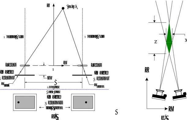
Photogrammetry is a three-dimensional coordinate measuring technique that uses photographs (images) acquired from still or video cameras. Gruen [6] uses the term videogrammetry to describe photogrammetry performed on video sequences. The authors will use photogrammetry throughout this paper. In its simplest form, a feature is observed from two distinct views and the two corresponding lines of sight are intersected in space to find a three-dimensional coordinate (forward intersection). The fundamental principle used by photogrammetry is in fact triangulation. Theodolites use the same principle for coordinate measurement. Figure 1 illustrates this principle in two-dimensional space. Incidentally, this two-camera arrangement is also called stereoscopy. In actual situations where the measuring chain is not perfect (poor image contrast, noise, etc.), many images from different views must be acquired in order to minimize the three-dimensional coordinates uncertainties. Furthermore, for a moving structure, the image sequence from different cameras must be synchronized together.
Image Sensor Lens Lens Image Sensor O Z X Optical Axis Optical Axis B F Xleft X right (X,Z) Image Sensors left - right Back view Top view
a)
Z
X
δz
δx
b)
Figure 1. Basic stereoscopic geometry for in-plane targets: a) forward intersection of light rays corresponding to a target, b) schematic diagram showing qualitatively the in-plane error shape. Let us study a simple stereoscopic arrangement where the camera model is based on the central perspective projection model, i.e., the pinhole model. The lens has no distortions and can be replaced by a pinhole where all the light rays pass through. With reference to Figure 1, one can draw a light-of-sight from point (X, Z) in the OXZ plane through the lens onto the image sensor both left and right. Assuming equal focal lengths F (or focus distance) for both imaging devices, one can extract the coordinate of the point (X, Z) lying in the OXZ plane,
right left right left X X X X B X − + = 2 Equation 1 and right left X X F B Z − = Equation 2
where B is the camera baseline. These two equations are expressed in terms of the so-called stereo disparity (Xleft - Xright). Before we derive the uncertainty equations, let us stop a moment on Figure 1b. This
figure depicts how errors in detecting the centroid of a particular target on the image sensor of the stereoscopic system produce errors in determining the location of the target in object space (δx,δz). The
uncertainty is not a scalar function of distance to the target. In fact, to estimate the measurement uncertainty, one has to find either the actual joint density function of the spatial error (probability distributions) or approximate it by applying the law of propagation of errors. The latter is applied to Equation 2, the resulting uncertainty along Z is
s
Z
F
B
p
z
xδ
δ
≈
2 Equation 3where px is the pixel size (typically 4-12 µm) and δs is the uncertainty in the stereo disparity in units of
pixels (e.g. 1/10 pixel). To get higher accuracy (lower uncertainty δz) one needs a large baseline, a higher
focal length, shorter distance camera-target and a low disparity measurement uncertainty. With increased focal length, the field of view becomes narrower. Too wide a baseline creates occlusions. Obviously, a larger image sensor, more images with a good distribution around the scene can alleviate these difficulties. The error along the X-axis is a linear function with the distance Z. A more complete camera model and exhaustive error representation can show that the error distribution is skewed and oriented with the line of sight.
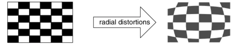
Camera model is covered by Atkinson [7]. This reference gives the details of the collinearity equations for the three-dimensional case where both internal (focal length, scaling, distortions) and external (matrix containing both rotation and translation information of a camera) parameters of a multi-camera arrangement are considered. Actual lenses have optical aberrations. Only optical distortions are modeled in photogrammetry. For instance, radial lens distortion can create the so-called barrel distortion effect (see Figure 2). The complete system of equations can be solved by the bundle adjustment method. This process evaluates both the coordinates of targets and external parameters using least squares based on collinearity equations. If the interior parameters are not available prior to this step (through an adequate camera calibration), a self-calibrating bundle adjustment is used.
radial distortions
Figure 2. Effect of radial distortions with real lenses, barrel distortions.
An extension of photogrammetry applies when the structure is rigid and the coordinates of feature points are known. In this particular case, one can extract the pose (camera orientation or external parameters) from a single camera arrangement. This is known as image resection. In our case, this can’t be applied because the structure is indeed non-rigid.
TECHNOLOGY AVAILABLE FOR OPTICAL METHODS
In this section, we look at the image recording technology available for close-range photogrammetry. Only digital photogrammetry is considered here because the inherent advantage in terms of flexibility and automation that this technology offers over graphical, analog and analytical photogrammetry.
Synchronized interlaced CCD or CMOS image cameras
These video cameras mimic the video standard used for broadcast television. An image is divided into two interlaced fields that when combined together on a TV-monitor guaranties flicker free viewing. Frame rates are 30 Hz for monochrome RS-170 (NTSC), 29.97 Hz for color RS-170A (NTSC) and 25 Hz for CCIR (PAL mono and color) video systems. Typical resolution of a RS-170 camera can vary but are typically 768 by 492 pixels. The major disadvantage for metrology applications is that a moving target is seen differently from the odd and even fields. This gives rise to the jagged edge effect. Therefore, only half the available resolution in the vertical direction is obtainable for three-dimensional coordinate measurement. External synchronization (GENLOCK) is possible on a number of models on the market.
Synchronized progressive scan cameras
These cameras read each pixel in the image without the interlaced technique. They were designed for high image acquisition quality and not display on a TV set. Progressive scan cameras are the preferred choice for digital photogrammetry. The combined cost (camera and frame grabber) is higher compared to the interlaced type cameras. Recent technological progress especially in the field of CMOS sensors, have created excellent products with high resolution and high frame rates, e.g. Basler A500 series, progressive Scan CMOS, 1280 X 1024 pixels, 500 frames/s with Camera Link interface. More progressive scan cameras are being produced with the IEEE-1394b, which does not require a frame grabber. With current digital interface standards, data rates limit cable lengths though repeaters can be used.
Analog/Digital video Camcorders
Most of these cameras are based upon the interlaced TV standard. They have the same characteristic as their counterpart with the difference that the analog image signal is recorded on a magnetic tape by an analog or digital (e.g. mini-DV) process.
Multiple digital still cameras
In recent years, these cameras have gained in popularity and have become the choice for taking photographs for many households. Professional models like the Kodak DCS Pro 14n packs more than 14 million pixels on a CMOS image sensor. They can be used for very slow motions or for documenting an earthquake site. By documenting, we mean calibrating the camera internal parameters (see discussion above) and using multi-station photogrammetry to extract features and build a three-dimensional model of a structure.
Recent technology aimed at digital electronic imaging
We skip web-cams and cellular phone video cameras because of the low quality optics and low image resolution. However, one could in case of necessity use them for documenting an event. Instead, we say a few words on recent technology. Cameras were for a long time made with CCD technology. Though this silicon technology provides high-quality image sensors, processing electronic can’t be added on the CCD sensor. The latest trend is now to use CMOS for image sensing [8]. This latter technology allows the combination of sensing and processing on the same chip (substrate). Smart cameras are now appearing on the market with capabilities like neural networks (ZiCam), RISC processor (ThinkEye), edge and shapes finding (Vision Components GmbH) and finally even Ethernet. For instance, with Ethernet capability, a set of cameras could be interconnected, programmed and results visualized from a single Web page. More development is needed before one sees such cameras being used for high-resolution photogrammetry.
EXTRACTING METRIC INFORMATION FROM ANALOG TAPES Available information
The post-experiment photogrammetric techniques were applied on the analog videotapes that were recorded during the shake table testing of a full-scale woodframe house [2]. Prior to the experiment, a theodolite survey was performed on the house. This piece of information was crucial in order to calibrate the lens of the cameras. Had the survey not been done, plans of the structure and image scaling techniques like those presented by D’Apuzzo et. al. [1] would have had to be used instead. Furthermore, two important targets for the present analysis were not surveyed well and hence high-resolution still images taken prior to the experiment were used to detect them and correct their values. Photogrammetry was possible with those still images because they were taken with the proper stereo convergence.
Retro-reflectors were installed so the theodolite survey could be done. These reflect light very efficiently back to the light source, e.g. typically they are 100 times more efficient at returning light than a
conventional target. A low-power light source located near the camera could have been used. The resulting images of the targets would have been very bright and easy to measure.
Woodframe house on uniaxial earthquake simulation system
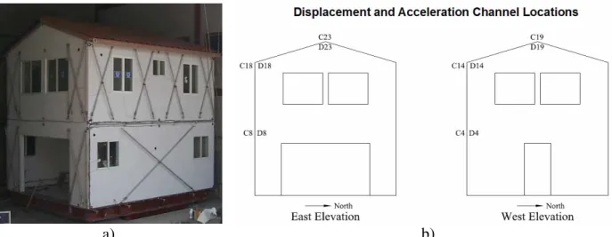
Figure 3a shows the east-north wall of the woodframe house. The contrast targets surveyed are visible on the image. Figure 3b shows some of the sensors locations on the east and west (not visible to the video cameras) elevations.
a)
b)
Figure 3. Test structure subjected to an earthquake ground motion during a shake table experiment a) photograph taken with a still camera showing the walls available for the study (some of the targets used for the photogrammetry are clearly visible), b) some of the sensors locations.
Video cameras and analog tapes
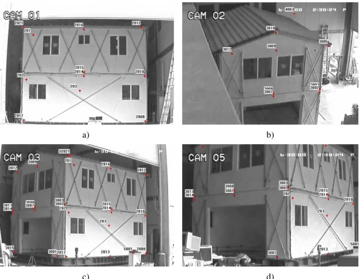
The video recordings were done with a set of ICD-703W cameras from Ikegami equipped with 8-mm Tamron CCTV lenses. During the shake table tests, the video signals were recorded on S-VHS analog videotapes. The tapes were converted to AVI digital files has soon as they were received. Unfortunately, the tape for CAM 02 (see Figure 4b) was damaged and a low quality signal was extracted. The video signals were synchronized together on the same time stamp. The timing information recorded on the upper right corner of the video images was of little use on the cassettes because they indicated units of seconds instead of frame number and two camera views had their upper right corner saturated by the ambient light (see Figure 4a, c). A weak light source pointed towards the retro-targets could have eliminated this problem because the images could have been under-exposed but the targets not. Hence, the time stamp would have appeared properly. Other types of man-made features (targets) could have been made, e.g., bright LEDs or pattern projection for real-time three-dimensional shape extraction [11].
a)
b)
c)
d)
Figure 4. Snapshots from the four video cameras used to extract the coordinates of the targets a) camera 1 (CAM 01) facing the north elevation, b) camera 2 (CAM 02) located above the house facing east elevation, c) camera 3 (CAM 03), d) camera 5 (CAM 05).
Calibration of the video cameras used for the earthquake simulation
The targets surveyed with the theodolite and still camera were used to calibrate the internal parameters of the ICD-703W video cameras. Figure 4 shows the different camera views along with the target locations.
Calibration with the commercial software ShapeCapture
The software ShapeCapture [9] was used to calibrate the cameras. The full photogrammetric camera model was applied. Figure 5 gives the camera parameters for CAM 03 and CAM 05. The first sixth parameters give the pose of the camera with respect to the target coordinate system. Then comes the focal length (close to the nominal value of 8 mm), the principle point of the image (Xo,Yo), affine image parameters to correct for scale difference and non-perpendicularity of the image coordinates (A,B), radial lens distortion parameters (K1 third and K2 fifth order), and, decentering lens distortion parameters (P1,P2).
a) b)
Figure 5. Camera calibration results assuming full camera model, a) parameters of CAM 03, b) parameters of CAM 05.
Effect of lens distortions on accuracy
To show the effect of lens distortions, forward intersection was applied to CAM 02 and CAM 05 for two cases. The first case assumes only radial distortions (see Figure 6a) and the second used the full model (see Figure 6b). It is clear that the cameras need the full photogrammetric camera model. Incidentally, this camera configuration gives the best results because according to Equation 3, one sees that errors are reduced if the baseline is wide and the distance camera-target is small. This is not the case for CAM 01 and CAM 03 combination. Notice the error on target 3012 located in the upper left corner of CAM 05; an area where distortions are maximum.
a) b)
Figure 6. Comparison of camera calibrations – simple versus full model, a) forward intersection of Cam 02 & 05 assuming strictly radial lens distortions, b) same but with full camera model. Snap-shots taken from the software ShapeCapture.
Target extraction and computation of target coordinates
Once the calibration is known, we can compute an estimate of the coordinate uncertainty. Table 1 shows the spatial resolution for a 1-pixel error in image coordinate as a function of camera-target distance. For instance, at a distance of 10 m, the errors are in the order of 10 mm.
Table 1. Expected spatial resolution for F=8 mm, B=6000 mm, px=6.6 µm and ∆ =1 pixel.
Z (mm) ∆X (mm) ∆Z (mm)
10000 8.25 13.75
A number of computer vision algorithms for target extraction were tested for the video sequences. Owing to the poor quality of the signals in the video sequences, all gave a resolution of ±0.5 pixel (in the image space). Usually one can expect 1/5 to a 1/10 of a pixel resolution according to Beyer [10]. The poor quality was due in part to target contrast (scene illumination), noise, frame grabber horizontal synchronization and scene occlusions. The loss of vertical resolution due to the interlaced video standard on the cameras did not have a great impact because vertical motion was very limited. The measured
resolution of ±0.5 pixel corresponds to about ±6 mm in object space (mainly horizontal). Apart from the
difference in sampling rate between electro-mechanical transducers (200 Hz) and video (29.97 Hz), the results of the photogrammetry will show plateaus as opposed of quasi-continuous waveforms.
In order to compute the target coordinates with forward intersection, the sequences had to be synchronized together. A few possibilities are available for the synchronization. One can use sound (clapper, voice, buzzer), a visual cue (flash) and the actual waveforms. Electronic means are the better way to go. For instance, the generation of a global image synchronization for both acquisition and digitization. If this latter option is not available then the other ones must be studied for accuracy before being used. We opted for the actual waveforms. A cross-correlation between two sequences followed by a peak detection based on a finite impulse response digital filter was used. The results from computing the target coordinates are presented in the following section.
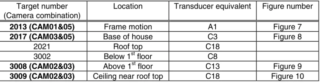
Table 2. Target number, description and corresponding sensor mounted on the house.
Target number (Camera combination)
Location Transducer equivalent Figure number
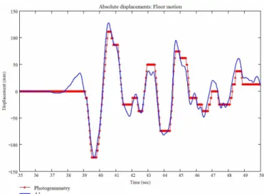
2013 (CAM01&05) Frame motion A1 Figure 7
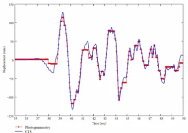
2017 (CAM03&05) Base of house C3 Figure 8
2021 Roof top C18
3002 Below 1st floor C8
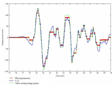
3008 (CAM02&03) Above 1st floor C13 Figure 9
3009 (CAM02&03) Ceiling near roof top C18 Figure 10
RESULTS
Table 2 gives the partial list of targets that were extracted with the method explained earlier. For each target, the closest transducer was picked. For example, target 3008 located above the first floor has its closest transducer situated at about 2.4 m behind it (at the back of the house). The assumption is that they move together. The four graphs that follow are indicative of the results of the absolute displacements obtained with photogrammetry on the analog videotapes.
Figure 7. Target 2013 extracted from CAM 01 and CAM 05.
Figure 8. Target 2017 extracted from CAM 03 and CAM 05.
Figure 10. Target 3009 extracted from CAM 02 and CAM 03.
DISCUSSION
To extract metric information, a linear image-to-space transformation or in other words a transformation from pixel to distance in the scene was tested. Target 3008 on CAM 02 was used as an example. To establish the linear transformation, the ratio of the distance between targets 3003 and 3008 on the house (provided by the survey) to the same distance measured in pixels on the image of CAM 02 was computed. The ratio (linear transformation) gave 14.2 mm/pixel. This scaling factor was applied to the image
coordinate in the horizontal direction (displacement of less than ±10 pixels). The result is shown on
Figure 11 where the curve obtained from linear transformation (pure pixel scaling) was superimposed on the curves of Figure 9. The resulting curve is close to the photogrammetric results. Still, photogrammetry gave slightly better results.
Relative displacements on the house could not be compared to measurements with photogrammetry because they needed a resolution of an order of magnitude below the current resolution. The current resolution is ±6 mm but a resolution below ±0.6 mm would have been necessary considering that relative
displacements measured with the electro-mechanical transducers are within ±15 mm. To achieve this type
of resolution with the current camera set-up, one would have to use a progressive scan camera with an industrial grade frame grabber (improved resolution by a factor 2), retro-targets (improved resolution by a factor 2 to 4) and at least 60 Hz cameras. Further improvements would come from the use of twice the current image sensor resolution (1280 by 1024 pixels), speed (100 Hz), and, maybe longer focal length (2X) at the cost of reducing the camera field of view. A reduced field of view is not a problem because as demonstrated in this experiment, a very small section of the image sensor is used to measure
displacements (about ±10 pixels). Baseline can’t be change because of the tight space around the
simulator. Finally, multi-station photogrammetry can be used to reduce the uncertainties in the measuring chain by way of measurement redundancy.
Figure 11. Example of linear image-to-space transformation, i.e., from image pixel to scene distances. The curve resulting from the linear transformation is superimposed on the curves for target 3008 (see Figure 9).
CONCLUSION
The paper showed how heterogeneous visual data sources can support the analysis of three-dimensional dynamic movement of a flexible structure subjected to an earthquake ground motion during a shake table experiment. In particular, the use of photogrammetric and computer vision techniques was illustrated by performing a post-experiment analysis on analog video tapes that were recorded during a shake table testing of a full-scale woodframe house on an uniaxial earthquake simulation system.
A review of real-time optical three-dimensional measurement techniques was presented in the context of shake table tests. Insights were presented for both physical aspects of the measurement process and on the technology available on the market. During a shake table experiment or any other similar event, visual information taken even without any specific analysis purpose (amateur’s pictures, video from a local TV station, analog videotapes) might be a meaningful source of information for subsequent spatial analysis. When ever possible, the right imaging equipment must be used. Current technology allows visual data to easily multiply (at an acceptable resolution) the number of locations on the structure where useful information can be extracted. By extension, a homogeneous distribution of those locations brings more robustness to monitoring such a structure. Future improvement in the technology (CMOS image sensors, interconnection, software, system integration) and testing of it should bring down the costs and make the technology available to a wider group of users.
REFERENCES
1. D’Apuzzo N., Willneff J. "Extraction of Metric Information from Video Sequences of an Unsuccessfully Controlled Chimneys Demolition". Proceedings of Optical 3-D Measurement Techniques V, Vienna, Austria, 2001: 259-265.
2.
Filiatrault, A., Fischer, D., Folz, B., and Uang C-M. “Seismic Testing of a Two-Story
Woodframe House: Influence of Wall Finish Materials”, ASCE Journal of Structural
Engineering, 2002, 128(10): 1337-1345.
3. Gruen A., Remondino F., Zhang L.. "Computer Reconstruction and Modeling of t he Great Buddha of Bamiyan, Afghanistan". The 19th CIPA International Symposium 2003, Antalya, Turkey, Oct. 2003: 440-445.
4. El-Hakim S. F. "Three-dimensional modeling of complex environments". SPIE Proceedings vol. 4309, Videometrics and Optical Methods for three-dimensional Shape Measurement, San Jose, Jan 20-26, 2001: 162-173.
5. Technologies for three-dimensional measurements: www.simple3D.com
6. Gruen A. "Fundamentals of videogrammetry – A review". Human Movement Science; 1997 (16): 155-187.
7. Atkinson K.B. "Close range photogrammetry and machine vision". Cathness, U.K.; Whittles, 1996. 8. Imaging web sites: www.advancedimagingmag.com, www.imagingsource.com
9. Commercial photogrammetry: www.shapecapture.com, www.optical-metrology-centre.com
10. Beyer, H.A. 1992. Geometric and radiometric analysis of a CCD-camera based photogrammetric close-range system. Ph.D. thesis, Institute of Geodesy and Photogrammetry, ETH Zurich, Switzerland, Mitteilungen No. 51.
11. Clarke, T.A. "An analysis of the properties of targets uses in digital close range photogrammetric measurement". Videometrics III, Boston, SPIE Vol. 2350. 1994: 251- 262.